Article

Prediction of Air-Conditioning Energy Consumption in R&D Building Using Multiple Machine Learning Techniques

1
Department of Civil Engineering, National Taiwan University, No. 1, Sec. 4 Roosevelt Road, Taipei 10617, Taiwan
2
Research Center of Climate Change and Sustainable Development, National Taiwan University, No. 1, Sec. 4 Roosevelt Road, Taipei 10617, Taiwan
*
Author to whom correspondence should be addressed.
Energies 2020, 13(7), 1847; https://doi.org/10.3390/en13071847
Submission received: 8 February 2020 / Revised: 3 April 2020 / Accepted: 4 April 2020 / Published: 10 April 2020
(This article belongs to the Section G: Energy and Buildings)

Abstract

:
With the global increase in demand for energy, energy conservation of research and development buildings has become of primary importance for building owners. Knowledge based on the patterns in energy consumption of previous years could be used to predict the near-future energy usage of buildings, to optimize and facilitate more effective energy consumption. Hence, this research aimed to develop a generic model for predicting energy consumption. Air-conditioning was used to exemplify the generic model for electricity consumption, as it is the process that often consumes the most energy in a public building. The purpose of this paper is to present this model and the related findings. After causative factors were determined, the methods of linear regression and various machine learning techniques—including the earlier machine learning techniques of support vector machine, random forest, and multilayer perceptron, and the later machine learning techniques of deep neural network, recurrent neural network, long short-term memory, and gated recurrent unit—were applied for prediction. Among them, the prediction of random forest resulted in an R2 of 88% ahead of the first month and 81% ahead of the third month. These experimental results demonstrate that the prediction model is reliable and significantly accurate. Building owners could further enrich the model for energy conservation and management.

Graphical Abstract

1. Introduction

The ongoing global economic development has increasingly consumed energy resource. Based on statistical Review of World Energy, global primary energy consumption grew rapidly in 2018, and at a rate of 2.9% last year, almost double its 10-year average of 1.5% per year, and the fastest since 2010 [1]. Moreover, according to the Stated Policies Scenario, electricity use has been growing at more than double the pace of overall energy demand, confirming its place at the heart of modern economies [2]. For the sake of sustainable development and mitigating the depletion of energy resources, energy conservation has become critical task during economic development.
The Ministry of Economic Affairs at Taiwan reported that the national electricity consumption in 2018 was about 264.3 billion kWh. The energy consumed by various buildings each year accounted for more than one-third of the national energy ratio, and the proportion grows year by year [3]. Therefore, the owners of public buildings with high electricity consumption [4] in Taiwan are often the main target for promoting public policies for energy conservation. The optimal operation of the buildings is crucial for reducing electricity consumption. Optimizing buildings’ electricity consumption will be more effective if the optimal operation can be used for estimating electricity savings based on data from the current usage and from previous years. Meanwhile, it is important to control the operation budget and the current expenditure. Thus, electricity saving would be realized and the estimation of electricity cost would be more realistic during the process of budgeting.
Taiwan is located in the transition zone corresponding to subtropical monsoon and tropical climates. The climate is characterized by longer periods of high temperatures in summer and shorter periods of low temperatures in winter. In Taiwan, the annual average temperature is 24.1 °C, and an annual sunshine total of 2180.8 h. This study used the Central Taiwan Innovation Campus (CTIC) of the Ministry of Economic Affairs as a demonstration site, because all of the R&D buildings of CTIC are typical public buildings.
CTIC categorizes the space in to five categories. They are office, research laboratory, pilot plant, conference for exhibition, training, conferences, library, and information exchange, and public service for restaurant, pantry, and parking facilities. Due to the need to perform various types of R&D projects, an R&D building often has a different project-base of occupants with different demands in terms of power resources. Consequently, it results in different power consumption rates. Therefore, the energy management process is highly complex, and energy-saving measures must be continuously deployed [5]. If the prediction of the electricity consumption in different rooms of the R&D building can be realized in the future, the predicted data will not only provide an optimized operation model for the building management team, but can also enable the occupants to benchmark their energy-saving goals.
The total electricity consumption of CTIC mainly comes from lighting, sockets, power usages, and air-conditioners. The changes in annual electricity consumption due to daylighting are not affected by the seasonal climate. The electricity consumption from sockets and power cannot be co-forecasted due to different models of usage. The electricity consumption of air-conditioners is easily affected by climatic factors in different months and seasons, and it accounts for 50% of the total energy consumption. If a more accurate modelling process for predicting electricity consumption can be constructed based on historical data, a more accurate energy-saving strategy and effectiveness evaluation can possibly be provided. If one could use the electricity consumption levels from previous years to predict near-future electricity usage, it would facilitate the more effective electricity consumption of buildings and form a better energy-saving strategy [6].
To predict building air-conditioning energy consumption, physical, semi-physical and data-driven methods are used. The physical and semi-physical methods estimate the energy demand of a building from geometrical information and thermal properties of the building [7]. However, the physical and semi-physical methods require a detailed understanding of building thermal dynamics to obtain several physical parameters [8]. By contrast, data-driven methods have been widely used to construct the air-conditioning energy consumption models due to their great processing capacity in solving nonlinear problems. They have taken sufficient account of the dynamic environments and future conditions [9]. The most popular data-driven method used in building energy consumption is linear regression (LR) [8], which is relatively simple to implement. However, LR is not suitable for non-linear problems and does not have self-learning ability. In recent years, machine learning (ML)—often used in the data science field—has been adopted to overcome such predicaments about energy management [10].
In general, ML includes the early evolved ML methods of multilayer perceptron (MLP) [11], support vector machine (SVM) [8], and random forest (RF) [10,11], and the more recently evolved MLs (namely deep learning (DL)) of deep neural network (DNN) [12], recurrent neural network (RNN) [13], long short-term memory network (LSTM) [14], and gated recurrent unit (GRU) [15]. Paudel et al. [8] used SVM with dynamic time warping pattern recognition methods to demonstrate that it uses adopted all available data for model training and has several drawbacks when applied to low energy buildings. Molina-Solana et al. [10] reviewed how data science has been applied in the field of energy management, such as MLP, SVM, an autoregressive movement average, and so on. Jang et al. [11] optimized a model for predicting the thermal energy consumption of a high school building by feature selection and MLP. Khalil et al. [12] proposed a DNN with eight inputs (relative compactness, surface area, wall area roof area, overall height, orientation, glazing area and glazing area distribution) to predicting the heating and cooling loads of a building based on a dataset for building energy performance. The DNN gives a very good prediction and the wall area, relative compactness and roof area have significant effects on heating and cooling loads. Mocanu et al. [13] presented five methods to predict energy consumption in a residential building, including DNN, or, more specifically, Conditional Restricted Boltzmann Machines and Factored Conditional Restricted Boltzmann Machines (FCRBM). The FCRBM is a powerful method which outperformed the other methods. Residential buildings over different time horizons with different time resolutions were discussed. Liu et al. [15] adopted four economic variables (gross domestic product (GDP), population, import and export trade volume, to forecast the primary energy consumption in China. Compared with MLP and SVM, GRU had the lowest average absolute percentage error.
This study is different from the aforementioned studies that generally focused on the electricity consumption of a whole building. In contrast, this study emphasizes exploring a framework to predict the electricity consumption for each room. The model provides a baseline of managerial mechanisms for facilitating effective energy saving. In order to construct a modelling process for a model for predicting the air-conditioning energy consumption of public buildings, the monthly electricity usage data of CTCI were collected to demonstrate the modelling processes of a generic model. The reader should be cautious that the emphasis should be on the modeling processes, not model itself, as well as on the exemplification, not on a CTCI case. The purpose of this paper is to present the research results based on the use of multiple ML techniques and to propose a generic modelling process for predicting electricity consumption. This research used experimental data measured in CTIC to construct a prediction model.
The paper begins with introducing CTIC, followed by the methodology used. Then, the modelling process is illustrated in detail. Next, the collected data are thoroughly analyzed and the accuracy and reliability of the proposed model are demonstrated. Finally, a conclusion is provided, and future research is recommended.

2. CTIC Background Information

2.1. Building Information

2.1.1. Location

CTIC is located in the Advanced Research Park of Central Taiwan (close to the center of Taiwan at 23°56′12.1″ N, 120°41′53.3″ E).

2.1.2. Mission and Main Functions

With strong government support, the Ministry of Economic Affairs expects CTIC to lead technological upgrades and job openings for small and medium enterprises in the region of central Taiwan. CTIC was constructed and is operated by the Industrial Technology Research Institute (ITRI) and opened on 15 September 2014. It covers a land area of 2.49 ha, with a total floor area of 42,000 m2, and it can also accommodate 700 people (400 for non-profit organizations and 300 for the information and communications technologies (ICT) industry). CTIC includes R&D space (office, research laboratory, and pilot plant), showroom and communication space (for exhibition, training, conferences, library, and information exchange), and public service areas (restaurant, pantry, and parking facilities); the design scheme and configured spaces are shown in Figure 1. CTIC hopes to transform into a high-level research and development park under the premise of maintaining the quality of urban life, and to combine with Central Taiwan Study and Research resources to promote local economic development. At present, about 87% of spaces have been stationed by various organizations.

2.1.3. Building Features

CTIC is a four-floor steel structure with one underground parking space. It is a low-carbon, energy-saving, sustainable ecological park, and aims to use energy-saving design as a basis for obtaining recognition as a highest-grade diamond-rating intelligent and green building in Taiwan.
There are quantifiable metrics for rating the green building and intelligent building. The rating of green building is also based on the subtropical climate of Taiwan. In reference to the core characteristics of the building in terms of energy consumption, water consumption, waste disposal and environmental protection, a set of assessment systems was developed.
The assessment system consists of nine indicators: (1) biodiversity, (2) base greening, (3) base water conservation, (4) daily energy saving, (5) carbon dioxide reduction, (6) waste reduction, (7) indoor environment, (8) water resources, (9) sewage and waste improvement. This system is the fourth in the world after the United Kingdom, the United States, and Canada, and is the fourth green building evaluation system with scientific quantification.
Assessor assigns different score points for each indicator. Then, the grade of green building badge would be given according to the sum of the score point which the assess gets. They are 5 grades: qualified grade (9–25 points), bronze grade (26–33 points), silver grade (34–41 points), gold grade (12–52 points), and diamond grade (53 points or more). CTIC got 59.74 points and Diamond Grade [16].
On the other hand, intelligent building emphasizes the application of smart technologies, such as networks, monitoring equipment and system integration, that can facilitate automatic sensing, analysis, and response functions as well as consider the convenience and optimal operation on future maintenance and management. Moreover, it has to meet user’s requirements for safety, comfort, demand for convenience and efficiency, and achieving the goal of energy saving. Eight indexes are used for evaluating the intelligent building. The indexes are integrated with wiring, information communication, system integration, facility management, safety and disaster prevention, health and comfort, thoughtful convenience, and energy-saving management. Each index score is 100 points. There are five grades, including qualified grade, bronze grade, silver grade, gold grade, and diamond grade; the highest diamond grade requires eight indicators all higher than 80 points. CTIC achieved higher than 80 points for each index and received diamond grade badge.

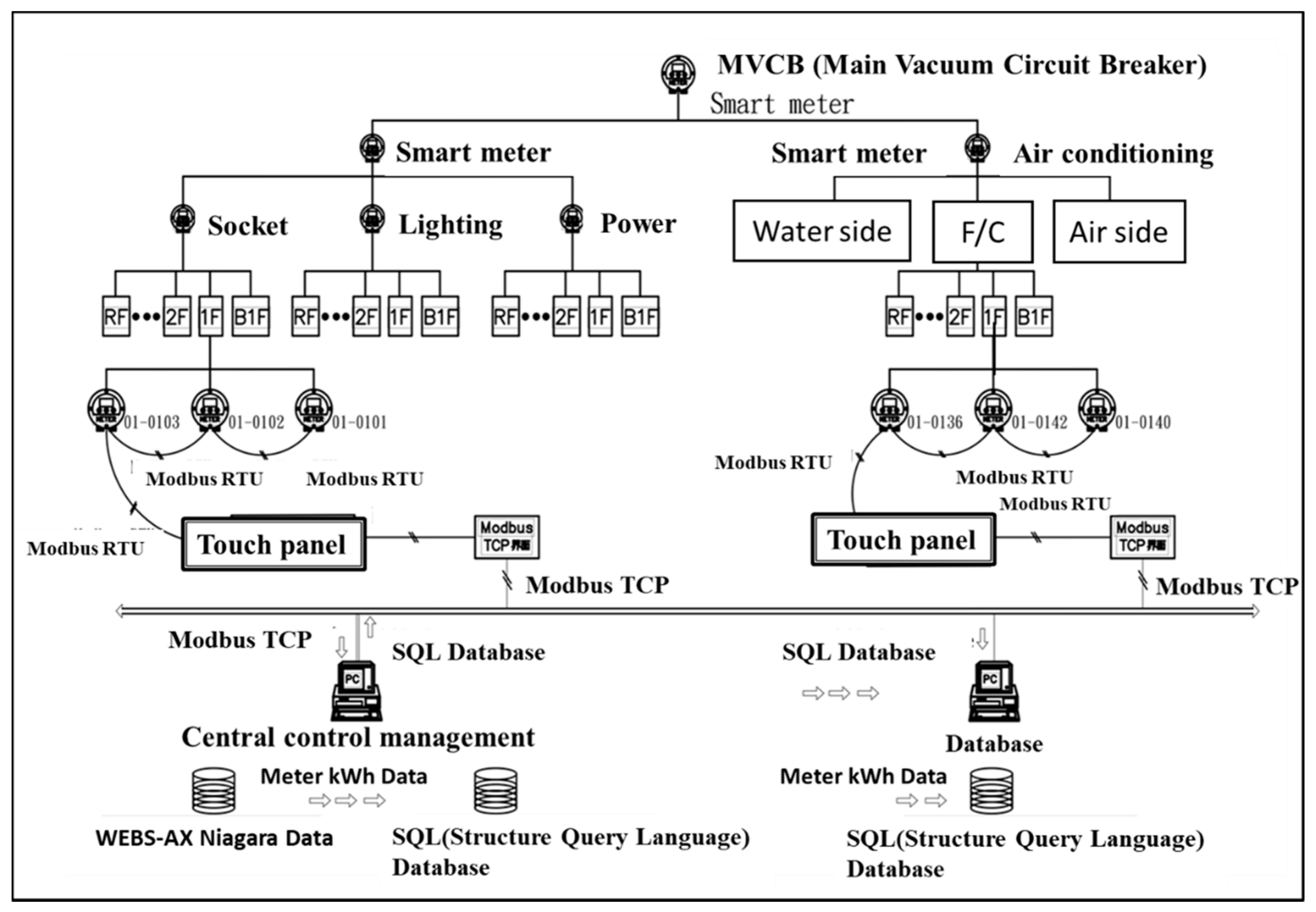
2.1.4. Building Energy Management System

CTIC explores two energy conservation strategies. The first is based on various spatial components (as shown in Table 1): If a building is a small city, from the city perspective, the more detailed division of space is more beneficial for building management because it is still inconvenient for the occupant’s daily life. R&D Buildings emphasize the interaction among different types of space users. It is difficult to manage energy consumption. Different types of spaces have different electricity supply and consumption rates due to differences in their usage, time of use, and associated equipment. The building energy management (BEM) system measures the electricity consumption of various types of spaces through detailed space division.
The second is based on the composition of each facility system (as shown in Table 1): In accordance with different space usages and the construction of each facility system, of which the air-conditioning system is the most complex and electricity-dissipative, the sum of each facility systems’ electricity consumption is equal to the power consumption of the entire building.
CTIC integrates the space management of the building information modeling (BIM) model and the smart grid system to construct a complete energy consumption monitoring system which can measure different electricity consumption rates from the lighting system, sockets, power, and air-conditioning devices in each room every hour. In order to provide good indoor environmental quality and to carry out the user-pays principle, detailed information and bills for the electricity consumption of each stationed unit are provided every month. This could be the basis for the continuous improvement of electricity conservation actions and to create an ecofriendly workplace.

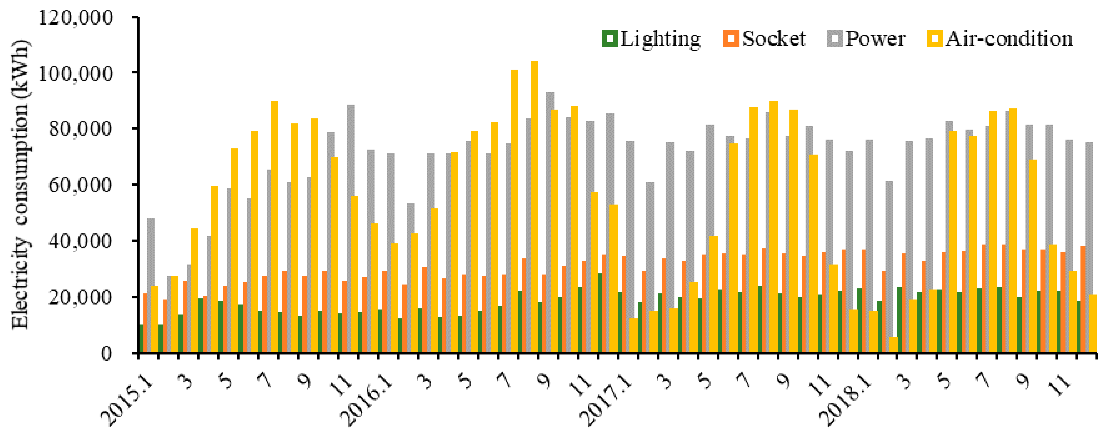
2.2. Electricity Consumption Data

Under the user-pays principle, and to maintain a comfortable working environment, CTIC sets up electric meters and independent electricity supply circuits for lighting, sockets, power, and air-conditioners in each room, and installs multifunction electric smart meters (as shown in Figure 2) to collect power consumption information. Thus, the energy management system can carry out various statistical analyses to strengthen electricity consumption management and achieve electricity-saving performance. In addition, the price of electricity can be calculated based on the actual electricity consumption of each stationed unit. With the exception of the user-pays principle, the stationed units can also strengthen the electricity-saving measures for continuous electricity-saving actions.
The space can be categorized into public spaces and independent spaces: research offices, laboratories, pilot plants, and conference rooms under the independent space category; lighting, sockets, power, and air-conditioning under the public space category. The electricity consumption statistics of the whole building from 2015 to 2018 are shown in the Figure 3. The electricity consumption rates of 383 rooms were collected across the time span from December 2014 to April 2019. The data consist of four types of facilities: lighting, sockets, power, and air-conditioning. The time spanned across 52 months and, thus, 79,664 monthly records of electricity usage data (383 × 4 × 52 = 79,664) were collected. These consumption data were used for the construction of the prediction model. Although the electricity consumption rates of 383 rooms were collected, the occupants of different projects and incubator normally move out of CTIC after the project ends. Therefore, this study selected 31 rooms with stable occupiers to predict electricity consumption. Table 2 shows the basic information of these 31 selected rooms.

2.3. Energy Consumption Factors

This study explored the six major factors affecting building air-conditioning energy consumption described in the relevant literature of the International Agency (IEA) for Energy in Buildings and Communities (EBC) Annex 53: climate, building envelope characteristics, building equipment, indoor environment, user behavior, maintenance mode, and social aspect-related factors [17].
This study explored the impact factors of building electricity consumption and selected 13 potential factors through multivariate statistical analysis. The selected factors were air pressure, temperature, humidity, wind speed, rainfall, sunshine hours, wet bulb temperature, season, month, area, floor, orientation, and the number of days of occupation. Among these factors, air pressure, temperature, humidity, wind speed, and rainfall were taken from the Nantou station of the Central Weather Bureau in Taiwan, and the hours of sunshine were taken from the Taichung station. The 13 factors were used for subsequently screening out electricity consumption factors through the grid search method. The detailed descriptions of each factor are as shown in Table 3.
As shown in Figure 4, the heat load zone of the building shell is divided into eight zones. The temperature changes of the external walls of the eight zones were measured and monitored. It was discovered that the measured results of the temperature changes in several zones are the same. Therefore, we combined the same result of the heat load zones into four zones, as shown in the middle of the Figure 4. In the lower right side of the Figure 4, one can see that the three zones marked in red color are high temperature zones with almost the same temperature. We group all three zones into one zone as the high temperature zone.

3. Research Methodology

This study used LR and multiple MLs, including earlier MLs and recent MLs, namely DLs, to construct an electricity consumption model to predict air-conditioning electricity consumption for the next 3 months.

3.1. Linear Regression

Linear regression is one of the most frequently used algorithms to achieve interpolating and extrapolation, the formula of linear regression can be formed as below,
y = X β + ϵ
In this equation, β and ϵ represents the p + 1 dimensional vector of coefficients and the set of n error terms, respectively. The ordinary least squares and maximum likelihood are the most commonly used algorithms to find out the coefficient β . For maximum likelihood, different likelihood estimates of β would be caused by the assumption about the underlying distribution of the error terms. According to the previous shortage, the ordinary least squares and inferential statistics reported which are based on the assumption that ϵ i ~ N   ( 0 ,   σ 2 ) iid for i = 1 to n, were employed in this study to estimate all linear regression.

3.2. Earlier Machine Learning

ML is the use of algorithms to classify collected data or predict training models. New data that are obtained in the future can be predicted through the training model [18].

3.2.1. Random Forest

Breiman (2001) [19] proposed the random forest (RF) algorithm, an ensemble learning method for ML. RF uses bootstrapping to build a large number of regression trees to form a forest and to ensure randomness by randomly selecting variables and sample prediction results. Regarding classification and regression, only sensitive parameters (the number of regression trees, the biggest feature m, and maximum depth) need to be determined [20]. A small number of parameters can simplify the problem, and RF has better prediction results than the traditional single-model without significant improvement of computational complexity. Peters et al. (2007) [21] used RF to establish an eco-hydrological environment model, and Naghibi et al. (2015) [22] used RF in conjunction with geographic information systems to map groundwater potential maps. Applying RF to establish potential collapse assessments has been widely used in recent years [11,23]. Building a RF can be divided into three steps, and this structure is shown in Figure 5.
The first step is randomization. The RF is combined by lots of condition inference trees, and to prevent high similarity between trees, RF imports bootstrapping to guarantee that the training data from each tree are not the same. Assuming that the data population has a total of K pieces of information, the model randomly chooses K times single datum, and each datum can be selected repeatedly as shown in the formula (2). It is valid with a sufficiently large K (K => ∞ theoretically). Therefore, the chance that a single datum is not selected can be calculated as follows [19]:
( 1 1 K ) K e 1 = 0.368
Those not-selected data are named as out-of-bag (OOB) data. The mean of OOB errors ( OOB ¯ ) is calculated to determine the parameters of RF and evaluate the sensitivity of inputs. The formula of the OOB ¯ error can be written as follows [19]:
OOB ¯ = 1 N i = 1 N ε i n L , i
where N represents the total amount of decision trees; ε i is the number of the misjudgment in i th decision tree; and n L , i is the total amount of OOB ¯ error in the i th decision tree. In general, the smallest N that can lead OOB ¯ to become stable and convergent might be the best decision tree quantity of RF.
Random sampling represents how many variables should be chosen for each decision tree. That is, before constructing a novel decision tree, the model would choose m variables as inputs from the all inputs M. According to the advice from Breiman (2001) [19], m can or can be decided as all inputs or the square root of all inputs (Sqrt):
m = M
After randomly selecting input variables and a subsample, a regression tree is established in second step for this subsample, and the process is repeated until the number of regression trees is satisfied, that is, until the construction of the RF model is completed.
After constructing the process of the RF, the testing data can be input into all of the decision trees in prediction step. Each decision tree calculates a single predicting value. The final prediction is the mean of all the prediction values of these decision trees.
An RF has three sensitive parameters (number of trees, the biggest feature, and maximum depth) that need to be calibrated for good performance. The basic concept of the grid search method is to evaluate all grid point indicators in the space, and then to determine the best factor and parameter combination after comparison. The grid search method [24,25] is simple, but has considerable computing resources. It is suitable for models with high computing efficiency. This method is used to determine the best hyper-parameters of the model, resulting in the highest test accuracy. The grid search was applied to find the best model parameters. The number of trees and maximum depth are continuous, so the number of trees varies from 50 to 1000 with spacing 50, and the maximum depth increases from 3 to 23. The biggest feature uses the setting of all inputs or Sqrt. Different combinations of the three parameters were examined, and the optimal combination of the model was determined.
The grid search method is a method for evaluating all grid points in space and finding the best performance. The structure of the grid search method can be divided into two parts: (1) Setting the upper and lower limits of the parameter—setting the range for searching the parameter, and the lower limit (l1) and upper limit (u1) of parameter 1 and the lower limit (l2) and upper limit (u2) of parameter 2. (2) Setting the grid size—setting the number of grids, dividing parameter 1 into equal p1, and the distance between the two grids is Δ p 1 = u 1 l 1 P 1 ; similarly, dividing parameter 2 into equal p2, and the distance between the two grids is Δ p 2 . Calculating the index of all of the grids is the way to determine the best-performing parameter combination. The total number of calculations is ( p 1 + 1 ) × ( p 2 + 1 ) . The calculation time will be longer if the searching range is larger or the grids are denser. This study selected several common parameters for a grid search.

3.2.2. Support Vector Machine

In the ML method, a support vector machine (SVM) is a supervised learning method. Vapnik developed SVM in the early 1990s to solve the problem of statistical classification [26]. In 1995, regression analysis also used SVM to solve this problem. SVM has two main characteristics. First, SVM uses structured risk minimization, which not only reduces the target error function but also considers the complexity of the network structure so that the model can reach a certain accuracy [27]. Thus, it will not make the structure so big as to increase computing time. Second, the weight of the structure and mode of the SVM model is transformed into a quadratic planning problem, which can be quickly solved using a standard algorithm [26,28]. SVM has been widely used in various fields in recent years, and has achieved quite good results in classification and forecasting. Four crucial parameters (kernel function, gamma, cost, epsilon, and degree) of SVM have to be determined [29]. These parameters influence the efficiency in handling the non-linear relationships and computational advantages, which are determined by the grid search method.

3.2.3. Multilayer Perceptron

The multilayer perceptron (MLP), proposed by Rumelhart et al. in 1986 [30], is a forward transfer-like neural network consisting of three layers of structure (input layer, hidden layer, and output layer), and uses the technology of back propagation to achieve supervised learning of model learning. The MLP consists of multiple node layers, each connected to the next layer. In addition to the input nodes, each node is a neuron with a nonlinear activation function [31]. Since MLP is a common neural network and has already been applied in research, further details of MLP can be found in related references.

3.3. Deep Learning

3.3.1. Deep Neural Network

The deep neural network (DNN) was proposed by Hinton in 2006 [32] to initialize the parameters using the restricted Boltzmann machine (RBM) to successfully solve the problem of backward transfer optimization and to make DL return to the front of the scene. However, as long as appropriate activation functions and sufficient training data are given, the benefits of the RBM method are not significant. Therefore, although the currently used DNN and MLP of the 1980s are similar in nature, they are still slightly different. In the 1980s, the network did not usually exceed three layers; however, the current network layer is often deeper than three layers. In the past, the sigmoid function was more commonly used as the activation function.
Because it is hard to obtain good results from the deeper network layers, this has been addressed through the use of rectified linear unit (Relu) in recent years [33].
In networks with deep training layers, the effect of Relu is much better than the sigmoid function. In addition, the training method is usually based on the stochastic gradient descent (Sgd) method [34]. When determining the best combination of weights in the network, the smaller the learning target, the better the optimized process. However, there are currently some new training methods. For example, the Adam algorithm can reduce the updating times of parameters during training and speed up the network to complete training earlier. The dropout algorithm randomly discards some neurons during training. Thus, the network performs better when it encounters data that it has never seen. Therefore, these methods can deepen the neural network to allow for the deep network. Consequently, it achieves the same task using less training data than the shallow network.

3.3.2. Recurrent Neural Network

The original prototype of the recurrent neural network (RNN) was proposed by Jeffrey L. Elman in 1990 [35], and it adds a recursive item into the neural network and takes the feedback of output values from hidden or output layer neurons as the message of the next input item. It memorizes the past information in the network through the recursive item so that the time information can be learned. The input of the RNN usually contains time series data, and the output value at the current time t is related to the output value of the previous time t − 1. The RNN also memorizes the information of the previous output value and stores the sequence data in a hidden layer. Each stage in the chain structure of the hidden layer can memorize the output value data of the previous stage and expand it. Time series data are inputted into x t , and at each time period in which data for x t are calculated in h t in the i-th stage, y t is outputted and a parameter w is given for the next stage. The prediction of building air-conditioning energy consumption is a time series problem. Thus, the RNN is suitable for forecasting the building air-conditioning energy consumption. The parameters, including hidden layers, activation, optimizer, batch, dropout, epoch and loss, is determined by grid search method.

3.3.3. Long Short-Term Memory

The long short-term memory (LSTM) was published by S. Hochreiter et al. in 1997 [36] to solve the problem of the traditional RNN, which is suitable for processing time series data. Even if the intermediate timing has a long interval, it avoids the problem of long-term dependence in design and has a good effect on identification. The difference from the traditional RNN lies in the internal chain structure of the hidden layer. The LSTM changes the neurons in the hidden layer to a set of recurrently connected subnets as memory cells. Each block contains self-connected neurons and three gates—input, output, and forget gates. Selective memory is performed by the input gate on the input value of this node, the output gate is used to determine whether the message is regarded as the output of this node, and the forget gate is to selectively forget the input value of the previous node [36]. The LSTM is one of RNN, which is suitable for time series data. The parameters, as with RNN, are determined by grid search method.

3.3.4. Gated Recurrent Unit

The gated recurrent unit (GRU) is also a variant of RNN. It proposed, by Cho et al. in 2014, to solve the problems of gradient disappearance and explosion similarly LSTM [37]. Its main structure is similar to LSTM in that it changes the neurons into memory blocks, and each block also contains self-connected neurons and gates. However, the GRU changes three gates into two by combining the input and forgotten gates into one update gate; thus, it does not have to decide if it forgets or inputs messages, and makes the decision at the same time. The other gate, the reset gate, determines the way to merge new input with previous messages. GRU also merges cell state and hidden state. It has fewer parameters than LSTM but still has the same effect; however, the calculation time is shorter than LSTM and it is easier to calculate [37]. The parameters of GRU is determined by grid search method. This study adopted the ML and DL techniques to construct model for predicting the building air-conditioning energy consumption using the Keras and Scikit-learning libraries in Python.

3.4. Model Constructing and Data Processing

The purpose of this study was to establish a general model for predicting air-conditioning electricity consumption and to provide a reference for regulating electricity consumption by collecting data from CTIC. This research used the information to operate data pre-processing including two procedures, data addendum and removing the extreme error. Data addendum demands that the missing value of the electricity consumption impact factor should be generated by interpolating. Besides, an R&D building often has different project-base of occupants with different demands in terms of power resources. Consequently, it results in different power consumption rates. All the data are automatically recorded through electricity meters. Those recorded extreme/abnormal data on electricity consumption near zero were removed from the training data set.
After completing data pre-processing, the aforementioned eight methods were used to establish a model, and then the grid search method was applied to find the optimal input factor and model parameters. The grid search method is used to determine the best hyperparameters of the model, resulting in the highest test accuracy, for example, the gamma in SVM, the number of trees in RF, and the number of hidden layers in MLP. As shown in Table 4, after cross-matching with the candidate combinations, the operation produces all of the results, and the evaluation index is then used to explore the goals and to pick the optimal model. The flowchart of the proposed method is shown in Figure 6. As shown in Figure 6, the framework of this research is demonstrated in the flowchart.
When constructing neural network (NN)-based models, collected data are usually partitioned into two parts—training and testing. The training materials are used for adjusting the parameters of the models, and the testing materials are then used to evaluate the model performance. This study analyzed the rooms in the building and partitioned training and testing according to different years. However, different assignments of training and testing may yield different results, and sometimes lead to different conclusions [29].
In terms of training and testing data, a model will be more accurate if the neural network uses more training data. Thus, this study referred to the data of 29 rooms from 2014 to 2017 (37 months) for training, and for testing, the data of 29 rooms from 2018 to 2019 (16 months). The remaining Room B318 and Room B114 were tested between 2014 and 2019. The ratio of training data to testing data is about 2 to 1 (a total of 1265 and 560). To further evaluate the prediction performance of the NN-based models, the root mean square error (RMSE) [38], mean absolute error (MAE) [39], determination coefficient (R2) [38], and coefficient of efficiency (CE) [39] were applied to this research, which indicates the discrepancy between observed and forecasted air-conditioning electricity consumption. RMSE and MAE represent the errors between two sets of data; meanwhile, R2, and CE represent the consistency between the observed and predicted air-conditioning electricity, and the greater the consistency, the better the results.

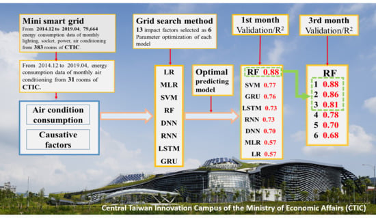
4. Data Analysis, Results, and Discussion

4.1. Factor Screening and Parameter Calibration

The factors and model parameters preferred by the grid search method are shown in Table 5 and Table 6. In terms of the model factors, the input factors of different models are slightly different, and most of the models perform the best with the combination of factors presented in Table 6. Therefore, this set of parameters was selected for subsequent model parameter calibration and future forecasting. The screened effective factors include the average temperature of the month, antecedent mean temperature, average humidity, air-conditioning energy consumption of the air conditioner, seasonal factors related to the time, and the area related to space, floor, and oriented factor. The changes in temperature and humidity can directly affect air-conditioning electricity consumption, and can also be deduced from seasonal factors. The final conditions of each room, such as area, floor, and orientation, are also effective factors affecting electricity consumption. Adding them to the model can increase its accuracy.
In terms of model parameters, the parameters selected by the SVM model perform better with the radial basis function (RBF) as the kernel function rather than the other three kernel functions (linear (LN), polynomial (PL), and sigmoid (SIG)). The RF model is stable at 350 trees, and obtains the best result if using the number of inputs as the maximum feature quantity and with a maximum depth of 22. The MLP model requires a large number of single-layer neurons and uses a limited-memory Broyden–Fletcher–Goldfarb–Shanno algorithm (Lbfgs) as an optimizer to get the best results. The number of hidden layers used in DL models such as DNN, RNN, LSTM, and GRU is greater than 2, which shows that the multiple hidden layers in DL models will be better than a single hidden layer. A network with recursive characteristics (RNN, LSTM, and GRU) also uses fewer layers than DNN, which means that the recursive network can use fewer neurons to store data. The remaining parameters are consistent with Rmsprop as the optimizer, Relu as the activation function, and MSLE as the loss, and no dropout layer is added.

4.2. Model Results and Comparison

After screening factors in this research, the prediction model of air-conditioning electricity consumption was constructed by six factors in eight models. Rigorous evaluation indicators were used to evaluate the performance of the model, and the air-conditioning electricity consumption predicted by the model output and the actual air-conditioning electricity consumption were analyzed in detail. This study firstly made a comparison among the LR, ML, and DL results for the following month to determine the differences in predictions of air-conditioning electricity consumption. The evaluation indicators for the prediction calculation of air-conditioning electricity consumption results for the following month are listed in Table 7. The table shows that the RMSE of the model in training and testing is lower than 404.7 kWh, and the R2 value is higher than 0.57. RF has the best performance, followed by GRU, RNN, DNN, LSTM, SVM, and MLP. The LR mode, however, has the worst performance. The RF test has the lowest RMSE and MAE values, and CE, and R2 indicators have the best performance. The value of CE can reach 0.75, while R2 can reach 0.88, which indicates that the model has 88% interpretive ability. DL falls from the second to fourth place. This may be because there is too little collected training data (1265 pieces) for training such a complex DL model and, hence, the training level is not strong enough to represent the advantages of DL.
The prediction results of air-conditioning electricity consumption during the next month are shown in Figure 7. All models can capture the changes in electricity consumption during the next month. The predicted values are very close to the observed values, especially when the values are below 3000 kWh (highlighted in Figure 7b). However, as shown in Figure 7c, some models cannot capture the peak value of the Room B114 test plant (about 10,000 kWh). The RF and DNN models can accurately predict the peak value of the Room B114 test plant, followed by the LR, SVM, and MLP modes. In addition, some models (MLP, RNN, and LSTM) report negative values at the minimum value and, thus, the vertical axis does not start from zero, and the negative values with little error are still acceptable.
Based on the results above, RF shows the best performance without negative values. It is more accurate than the other models regarding peak and small values. The modeling process of RF is illustrated in Figure 8. Therefore, the RF model was used for predicting the electricity consumption during the following 6 months. Its parameters and inputs are shown in Figure 8.

4.3. Prediction

From the previous chapter, it can be seen that RF is the best model for predicting the electricity consumption of air-conditioning. Therefore, the RF model was used to predict the electricity consumption in the following 6 months as a basis for energy conservation. Table 8 presents the evaluation indicators of the RF model forecast results. It shows that the forecasting time of the error indicators (RMSE and MAE) increases. As the error gradually grows, the trend indicators CE progressively worsen. The analytical capability, R2, also deteriorates. Despite this, the model predicts that the RMSE of the next 6 months will be only 363.3 kWh (47.4% of the observed mean electricity consumption of air-conditioning), and CE will start to become negative after the forecast of the next 3 months, but R2 still has a level of 0.81.
However, it still maintains a certain accuracy. Furthermore, the CE value of RF is predicted to be 0.52 in the following 2 months, but the CE value of the following 3 months is predicted to be −1.53, and the gap is too large. After reviewing the data, it was found that the room B445 has a small amount of electricity consumption with a small fluctuation, which results in the calculation of the averaged CE value becoming negative. If room B445 is removed, the calculated value of CE becomes 0.85, 0.74, 0.60, 0.59, 0.43, and 0.09 for 1- to 6-month-ahead predictions, respectively. This indicates that the performance of the remaining rooms is good, and the calculation error (RMSE and MAE) after removing room B445 is small, and R2 is still at the level of 0.81.
Figure 9 shows the air-conditioning electricity consumption in the following 6 months as predicted by the RF mode. The longer the prediction time, the worse the prediction results, but the trend can still be predicted. A room with lower electricity consumption performs better. Much lower electricity consumption is predicted for Room B114 with a large electricity consumption, and the longer the predicted time, the greater the predicted delay time. The results demonstrate that the RF model can provide quite reliable predictive information for the following 3 months. Figure 10 summarizes step-by-step procedures to obtain the reliability of R2 for the next 3-month prediction—0.88, 0.84, and 0.81—and provides better information on how to save energy and reduce carbon for relevant decision-makers.

5. Conclusions

In order to construct a generic modelling process for predicting the air-conditioning energy consumption of public buildings, nearly 79,664 monthly records of electricity usage data were collected to construct the generic model. Meanwhile, the grid search method was employed to calibrate the model parameters. Consequently, six valid factors were selected from the 13 factors. They were temperature, humidity, season, area, floor, and orientation. These factors significantly affected the change in the electricity consumption of air-conditioners. Based on these parameters and factors, the methods of linear regression and the ML techniques of various ML and DL approaches were applied and compared. These methods included LR, SVM, RF, MLP, DNN, RNN, LSTM and GRU.
The overall results show that the RF produces the best prediction of electricity consumption with the smallest RMSE and highest CE. Its R2 for predictions in the first month was 0.88. Moreover, the prediction for the third month was 0.81. Thus, the reliability and accuracy of the constructed model in predicting the air-conditioning electricity consumption for the next 3 months were demonstrated. Nevertheless, the prediction model proposed in this research could be limited to the same type of building, i.e., public R&D buildings of CTIC in Taiwan. To avoid potential pitfalls, the model may not be applicable when different spaces in different buildings are considered. To enhance the model, the continuous collection of electricity consumption data from different types of buildings is necessary in future research. Thus, a more generic and robust model could be constructed to provide much more reliable information to aid decision making in energy conservation and management.

Author Contributions

All the authors have participated in the research as following contributions: conceptualization & main ideas, J.-M.L. and L.-M.C.; literature review, J.-M.L. and M.-J.C.; research framework, J.-M.L., M.-J.C. and L.-M.C.; data curation, J.-M.C. and L.-M.C.; data collection, J.-M.L.; machine learning and linear regression modeling M.-J.C. and J.-M.L.; data analysis and validation, M.-J.C., J.-M.L. and L.-M.C.; writing-original draft preparation, J.-M.L. and M.-J.C.; editing and response to reviewer’s comments, M.-J.C. and J.-M.L.; writing-final review, L.-M.C. All authors have read and agreed to the published version of the manuscript.

Funding

Research was sponsored by High-Tech Facility Research Center, Department of Civil Engineering, National Taiwan University (TLIRC-CI43).

Conflicts of Interest

The authors declare no conflict of interest.

Abbreviations

OrderAbbreviationFull Form
1BEMBuilding energy management
2BIMBuilding information modeling
3CCCorrelation coefficient
4CECoefficient of efficiency
5CTICCentral Taiwan Innovation Campus
6DLDeep learning
7EBCEnergy in Buildings and Communities
8GRUGated recurrent unit
9ICTInformation and communications technologies
10IEAInternational Energy Agency
11ITRIIndustrial Technology Research Institute
12LbfgsLimited-memory broyden–fletcher–goldfarb–shanno algorithm
13LNLinear kernel fuction
14LSTMLong short-term memory
15MAEMean absolute error
16MLPMachine learning
17MLPMultilayer perceptron
18MSLEMean squared logarithmic error
19NNNeural network
20OOBOut of bag
21PLPolynomial kernel fuction
22R&DResearch and development
23R2Determination coefficient
24RBFRadial basis function kernel function
25RBMBoltzmann machine
26ReluRectified linear unit
27RFRandom forest
28RMSERoot mean square error
29RMSpropRoot mean square propagation
30RNNRecurrent neural network
31SgdStochastic gradient descent
32SIGSigmoid kernel fuction
33SqrtSquare root of a number of inputs

References

  1. British Petroleum. Statistical Review of World Energy. p. 2. Available online: https://www.bp.com/content/dam/bp/business-sites/en/global/corporate/pdfs/energy-economics/statistical-review/bp-stats-review-2019-full-report.pdf (accessed on 1 March 2020).
  2. International Energy Agency (IEA). World Energy Outlook 2019. Available online: http://www.worldenergyoutlook.org/ (accessed on 1 March 2020).
  3. Ministry of Economic Affairs Bureau of Energy. Ministry of Economic Affairs 2019 Annual Report; Taiwan. Available online: https://www.moea.gov.tw/MNS/english/home/English.aspx (accessed on 1 March 2020).
  4. Architecture and Building Research Institute. Collaborative research project on innovative low-Carbon green building environmental technology plan–Research on Guiding Principles of Sub-metering Design of Building Electricity System; Architecture and Building Research Institute: New Taipei City, Taiwan, 2015; p. 1. [Google Scholar]
  5. Cho, S.; Lee, J.; Baek, J.; Kim, G.S.; Leigh, S.B. Investigating Primary Factors A_ecting Electricity Consumption in Non-Residential Buildings Using a Data-Driven Approach. Energies 2019, 12, 4046. [Google Scholar] [CrossRef] [Green Version]
  6. Zhou, J.; Huo, X.; Xu, X.; Li, Y. Forecasting the Carbon Price Using Extreme-Point Symmetric Mode Decomposition and Extreme Learning Machine Optimized by the Grey Wolf Optimizer Algorithm. Energies 2019, 12, 950. [Google Scholar] [CrossRef] [Green Version]
  7. Underwood, C.P.; Yik, F.W.H. Modeling Methods for Energy in Buildings; Blackwell Science: Oxford, UK, 2004. [Google Scholar]
  8. Paudel, S.; Elmitri, M.; Couturier, S.; Nguyen, P.H.; Kamphuis, R.; Lacarrière, B.; Le Corre, O. A relevant data selection method for energy consumption prediction of low energy building based on support vector machine. Energy Build. 2017, 138, 240–256. [Google Scholar] [CrossRef]
  9. Kristopher, T.W.; Juan, D.G. Predicting future monthly residential energy consumption using building characteristics and climate data: A statistical learning approach. Energy Build. 2016, 128, 1–11. [Google Scholar]
  10. Molina-Solana, M.; Ros, M.; Ruiz, M.D.; Gómez-Romero, J.; Martín-Bautista, M.J. Data science for building energy management: A review. Renew. Sustain. Energy Rev. 2017, 70, 598–609. [Google Scholar] [CrossRef] [Green Version]
  11. Jang, J.; Lee, J.; Son, E.; Park, K.; Kim, G.; Lee, J.H.; Leigh, S.B. Development of an Improved Model to Predict Building Thermal Energy Consumption by Utilizing Feature Selection. Energies 2019, 12, 4187. [Google Scholar] [CrossRef] [Green Version]
  12. Khalil, A.J.; Barhoom, A.M.; Abu-Nasser, B.S.; Musleh, M.M.; Abu-Naser, S.S. Energy Efficiency Predicting using Artificial Neural Network. Int. J. Acad. Pedagog. Res. 2019, 3, 1–7. [Google Scholar]
  13. Mocanu, E.; Nguyen, P.H.; Gibescu, M.; Kling, W.L. Deep learning for estimating building energy consumption. Sustain. Energy Grids Netw. 2016, 6, 91–99. [Google Scholar] [CrossRef]
  14. Marino, D.L.; Amarasinghe, K.; Manic, M. Building energy load forecasting using deep neural networks. In Proceedings of the IECON 2016–42nd Annual Conference of the IEEE Industrial Electronics Society, Florence, Italy, 24–27 October 2016. [Google Scholar]
  15. Liu, B.; Fu, C.; Bielefield, A.; Liu, Y.Q. Forecasting of Chinese primary energy consumption in 2021 with GRU artificial neural network. Energies 2017, 10, 1453. [Google Scholar] [CrossRef]
  16. Taiwan Architecture and Building Center. Grading Book; Taiwan; Available online: https://eewh.tw/ (accessed on 1 March 2020).
  17. Hiroshi Yoshino. Final Report Annex 53–Total Energy Use in Buildings–Analysis and Evaluation Methods; Institute for Building Environment and Energy Conservation: Kojimachi, Tokyo, 2013. [Google Scholar]
  18. Deb, C.; Zhang, F.; Yang, J.; Lee, S.E.; Shah, K.W. A review on time series forecasting techniques for building energy consumption. Renew. Sustain. Energy Rev. 2017, 74, 902–924. [Google Scholar] [CrossRef]
  19. Breiman, L. Random Forests. Mach. Learn. 2001, 45, 5–32. [Google Scholar] [CrossRef] [Green Version]
  20. Liu, C.B.; Chamberlain, B.P.; Little, D.A.; Cardoso, Â. Generalising random forest parameter optimisation to include stability and cost. In Joint European Conference on Machine Learning and Knowledge Discovery in Databases; Springer: Skopje, Macedonia, September 2017. [Google Scholar]
  21. Peters, J.; Baets, B.D.; Verhoest, N.E.C.; Samson, R.; Degroeve, S.; Becker, P.D.; Huybrechts, W. Random forests as a tool for ecohydrological distribution modeling. Ecol. Modell. 2007, 207, 304–318. [Google Scholar] [CrossRef]
  22. Naghibi, S.A.; Pourghasemi, H.R.; Dixon, B. GIS-Based groundwater potential mapping using boosted regression tree, classification and regression tree, and random forest machine learning models in Iran. Environ. Monit. Assess. 2016, 188, 44. [Google Scholar] [CrossRef] [PubMed]
  23. Pourghasemi, H.R.; Kerle, N. Random forests and evidential belief function-based landslide susceptibility assessment in Western Mazandaran Province, Iran. Environ. Earth Sci. 2016, 75, 185. [Google Scholar] [CrossRef]
  24. Brad, J.F. An efficient point algorithm for a linear two-Stage optimization problem. Oper. Res. 1983, 31, 670–684. [Google Scholar] [CrossRef]
  25. Zhao, L.; Zha, Y.; Zhuang, Y.; Liang, L. Data envelopment analysis for sustainability evaluation in China: Tackling the economic, environmental, and social dimensions. Eur. J. Oper. Res. 2019, 275, 1083–1095. [Google Scholar] [CrossRef]
  26. Vapnik, V.N. The Nature of Statistical Learning Theory; Springer: New York, NY, USA, 1995. [Google Scholar]
  27. Cristianini, N.; Shaw–Taylor, J. An Introduction to Support Vector Machines and Other Kernel-Based Learning Methods; Cambridge University Press: New York, NY, USA, 2000. [Google Scholar]
  28. Chang, M.J.; Chang, H.K.; Chen, Y.C.; Lin, G.F.; Chen, P.A.; Lai, J.S.; Tan, Y.C. A Support Vector Machine Forecasting Model for Typhoon Flood Inundation Mapping and Early Flood Warning Systems. Water 2018, 10, 1734. [Google Scholar] [CrossRef] [Green Version]
  29. Lin, G.F.; Chang, M.J.; Huang, Y.C.; Ho, J.Y. Assessment of susceptibility to rainfall-induced landslides using improved self-Organizing linear output map, support vector machine, and logistic regression. Eng. Geol. 2017, 224, 62–74. [Google Scholar] [CrossRef]
  30. Trigila, A.; Iadanza, C.; Esposito, C.; Scarascia-Mugnozza, G. Comparison of Logistic Regression and Random Forests techniques for shallow landslide susceptibility assessment in Giampilieri (NE Sicily, Italy). Geomorphology 2015, 249, 119–136. [Google Scholar] [CrossRef]
  31. Rumelhart, D.E.; Hinton, G.E.; Williams, R.J. Learning internal representations by backpropagating errors. Nature 1986, 323, 533–536. [Google Scholar] [CrossRef]
  32. Hinton, G.; Salakhutdinov, R. Reducing the dimensionality of data with neural networks. Science 2006, 313, 504–507. [Google Scholar] [CrossRef] [PubMed] [Green Version]
  33. Nair, V.; Hinton, G.E. Rectified linear units improve restricted boltzmann machines. In Proceedings of the 27th international conference on machine learning (ICML-10), Haifa, Israel, 21–24 June 2010. [Google Scholar]
  34. Bottou, L. Large-Scale machine learning with stochastic gradient descent. In Proceedings of the COMPSTAT’2010: 19th International Conference on Computational Statistics, Paris, France, 22–27 August 2010; pp. 177–186. [Google Scholar]
  35. Elman, J.L. Finding structure in time. Wiley Interdiscip. Rev. Cognit. Sci. 1990, 14, 179–211. [Google Scholar] [CrossRef]
  36. Hochreiter, S.; Schmidhuber, J. Long short-Term memory. Neural Comput. 1997, 9, 1735–1780. [Google Scholar] [CrossRef] [PubMed]
  37. Cho, K.; Van Merriënboer, B.; Gulcehre, C.; Bahdanau, D.; Bougares, F.; Schwenk, H.; Bengio, Y. Learning phrase representations using RNN encoder-Decoder for statistical machine translation. arXiv 2014, arXiv:1406.1078. [Google Scholar]
  38. Lin, G.F.; Chang, M.J.; Wu, J.T. A hybrid statistical downscaling method based on the classification of rainfall patterns. Water Resour. Manag. 2017, 31, 377–401. [Google Scholar] [CrossRef]
  39. Wang, J.H.; Lin, G.F.; Chang, M.J.; Huang, I.H.; Chen, Y.R. Real-Time water-Level forecasting using dilated causal convolutional neural networks. Water Resour. Manag. 2019, 33, 3759–3780. [Google Scholar] [CrossRef]
Figure 1. Design scheme and configuration space.
Energies 13 01847 g001
Figure 2. Smart meter system.
Energies 13 01847 g002
Figure 3. The electricity consumption of CTIC.
Energies 13 01847 g003
Figure 4. Orientation of the rooms.
Energies 13 01847 g004
Figure 5. The structure of the RF algorithm.
Energies 13 01847 g005
Figure 6. Flowchart of the proposed model.
Energies 13 01847 g006
Figure 7. Comparison of the predicted electricity consumption of (a) all rooms, (b) rooms below 3000 kWh, and (c) rooms above 3000 kWh with 1-month-ahead predictions of eight models in the testing phase.
Energies 13 01847 g007
Figure 8. The RF structure with optimal parameters and inputs.
Energies 13 01847 g008
Figure 9. Comparison of the predicted electricity consumption with the (a) 1-, (b) 2-, (c) 3-, (d) 4-, (e) 5- and (f) 6-month-ahead predictions of the RF model in the testing phase.
Energies 13 01847 g009
Figure 10. Summary of procedures for 3-month-ahead predictions.
Energies 13 01847 g010
Table 1. Various spatial components.
SpacePublic Space (53.3%)Independent Space (46.7%)
Parking LotServiceOfficeLaboratoryPilot PlantConferenceTotal
Room12385965149383
Area (m2)613310,906600349871971196731,967
Table 2. Basic information of the selected 31 rooms.
OrderRoomFloor AreaFloorOrientationSpace CategoryMaximum Monthly Electricity Consumption
R1A11017511office2803.8
R2A31513631office4921.8
R3A3168431office2068.0
R4B22015823office2023.2
R5B2308022office1615.6
R6B2317622office1530.5
R7B2375324office1907.2
R8B30152031office6310.0
R9B3036334office568.0
R10B3045934office1331.7
R11B31816934office1842.7
R12B3294532office544.3
R13B4105644office1214.0
R14B4305743office1052.1
R15B4475244office281.4
R16A10816111laboratory1962.8
R17A12113811laboratory17,517.9
R18A3237534laboratory1090.3
R19A3248334laboratory1634.8
R20B2239323laboratory1978.1
R21B4087644laboratory1283.3
R22B4215244laboratory321.0
R23B4235641laboratory950.4
R24B4255041laboratory1052.1
R25B4398442laboratory822.4
R26B4413842laboratory1148.0
R27B4454942laboratory731.8
R28B4465342laboratory697.3
R29B10214911pilot plant1586.3
R30B1046711pilot plant1533.7
R31B11421711pilot plant9023.3
Table 3. The explanation of the causative factors.
CategoryFactorExplanation
Outdoor environmental factorAir pressureMonthly average pressure
TemperatureAverage temperature during monthly working hours (8:00–18:00)
HumidityAverage humidity during monthly working hours (8:00–18:00)
Wind speedMonthly average wind speed
RainfallMonthly average rainfall
Sunshine hoursMonthly average hours of sunshine
Wet bulb temperatureTemperature recorded by a thermometer that has its bulb wrapped in cloth and moistened with distilled water
SeasonSpring (March, April, May), Summer (June, July, August), Autumn (September, October, November) and Winter (December, January, February)
MonthJanuary–December
Building characteristicsFloor areaArea of each room
Floor locationGround, middle and roof
Orientation1, 2, 3 and 4
Use behaviorDays of useWorking days of the month
Table 4. The Candidate parameters of the models.
ModelParameter
SVMKernel functionGammaCostEpsilonDegree
RBF, LN, PL, SIG(2−7, 27, 2)(2−7, 27, 2)(2−7, 27, 2)(2, 3, 1)
RFNumber of treesMax feature
(50, 1000, 50)All inputs, Sqrt
MLPHidden layerActivationOptimizerBatchInitial learning rate
{[8]}, {[16]}, {[32]}, {[64]}, {[128]}, {[256]}, {[512]}Tanh, ReluAdam, Sgd, Lbfgs2000.001, 0.0001
DNN
RNN
GRU
LSTM
Hidden layerActivationOptimizerBatchDropoutEpochLoss
{[32]}, {[64]}, {[128]}, {[256]}, {[512]}Tanh,
Relu
Nadam,
Adam,
Rmsprop
32,
64,
128
80%,
90%,
100%
30,
50
MAE, MSLE
{[32], [64]}, {[64], [128]}, {[128], [256]}
{[32], [64], [128]}, {[64], [128], [256]}
{[32], [64], [128], [256]}, {[64], [128], [256], [512]}
{[32], [64], [128], [256], [512]}
Note 1: (n, m, d) represents a sequence of differences from the lower limit n to the upper limit m, and Rmsprop is root mean square propagation. Note 2: {[f], [s], [t]} indicates that there are three layers in total, and the number of neurons in the three layers is f, s, and t, respectively.
Table 5. The optimal input combinations of models determined by the grid research method.
InputLag Length
tt − 1t − 2
Monthly mean temperature111
Monthly mean humidity111
Season1
Floor area1
Floor location1
Orientation1
Air-conditioning electricity consumption111
Note: Monthly mean temperature and humidity are average values from 08:00 to 18:00, air-conditioning electricity consumption is the total amount per month, and the lag length t, t − 1, and t − 2 indicate the current time is t, one month before the current time is t − 1, and two months before the current time is t – 2.
Table 6. Optimal parameters of models determined by the grid research method.
ModelParameter
SVMKernel functionGammaCostEpsilonDegree
RBF20.50.00781
RFNumber of treesMax featureMax depth
350Number of inputs22
MLPHidden layerActivationOptimizerBatchInitial learning rate
{[256]}ReluLbfgs2000.0001
Hidden layerActivationOptimizerBatchDropoutEpochLoss
DNN{[32], [64], [128]}ReluRmsprop32100%300MSLE
RNN{[64], [128]}
GRU{[128], [256]}
LSTM{[32], [64]}
Note 1: (n, m, d) represents a sequence of difference stages from the lower limit n to the upper limit m. Note 2: {[f], [s], [t]} indicates that there are three layers in total, and the number of neurons in the three layers is f, s, and t, respectively.
Table 7. Comparison of the predicted electricity consumption with 1-month-ahead predictions of eight models in the testing phase.
ModelTraining PhaseTesting Phase
RMSEMAECER2RMSEMAECER2
LR404.7288.8−0.210.42309.8230.6−6.140.57
MLP272.9202.20.270.53267.5209−3.190.57
SVM352.4230.90.450.6246187.5−1.850.77
RF131.687.90.920.94189.8141.40.750.88
DNN157.5113.50.660.77239.5182.4−0.560.7
RNN150.3108.70.760.81221.5174.9−0.950.73
LSTM249.5175.70.490.63244190.2−0.450.73
GRU118.486.40.820.87202.3152.1−1.230.76
Note: The units of RMSE and MAE are kWh, means 1 kilowatt (1 kW) of power sustained for 1 h.
Table 8. RMSE, MAE, CE, and R2 values of the RF model for 1- to 6-month-ahead predictions in the testing phase.
Lead TimeTraining PhaseTesting Phase
RMSEMAECER2RMSEMAECER2
1131.687.90.920.94189.8141.40.750.88
2148.899.00.920.93230.5180.70.520.84
3157.4108.40.910.93267.6212.2−1.530.81
4156.2108.80.920.94269.6226.1−1.880.78
5160.2111.50.920.94337.6277.2−2.490.70
6163.0115.70.920.94363.3296.3−3.010.68
Note: The units of RMSE and MAE are in kWh.

