The Effect of Deep Energy Retrofit on The Hourly Power Demand of Finnish Detached Houses

Abstract

This study examines how the energy renovation of old detached houses affects the hourly power consumption of heating and electricity in Finland. As electrification of heating through heat pumps becomes more common, the effects on the grid need to be quantified. Increased fluctuation and peak power demand could increase the need for fossil-based peaking power plants or call for new investments to the distribution infrastructure. The novelty in this study is the focus on hourly power demand instead of just annual energy consumption. Identifying the influence of building energy retrofits on the instantaneous power demand can help guide policy and investments into building retrofits and related technology. The work was done through dynamic building simulation and utilized building configurations obtained through multi-objective optimization. Deep energy retrofits decreased both the total and peak heating power consumption. However, the use of air-source heat pumps increased the peak power demand of electricity in district heated and wood heated buildings by as much as 100%. On the other hand, peak power demand in buildings with direct electric heating was reduced by 30 to 40%. On the building stock level, the demand reduction in buildings with direct electric heating could compensate for the increase in the share of buildings with ground-source heat pumps, so that the national peak electricity demand would not increase. This prevents the increase of demand for high emission peaking power plants as heat pump penetration rises. However, a use is needed for the excess solar electricity generated by the optimally retrofitted buildings, because much of the solar electricity cannot be utilized in the single-family houses during summer.

1. Introduction

The European Union (EU) aims to reduce CO₂ emissions by 80% compared to 1990 levels by the year 2050 [1]. The EU recognizes electrification of heating through heat pumps as one key step towards decarbonization [2]. Since buildings are responsible for 40% of EU’s energy demand and emissions, the Energy Performance of Buildings Directive (EPBD) was created to reduce emissions caused by the operation of future buildings [3]. However, despite tightening regulation of new buildings, the existing energy-inefficient building stock that has mostly been built before modern regulations remains the biggest source of building-based emissions. To tackle this issue, the EU has called for national retrofit strategies to effect a positive change in the existing buildings as well [4]. Finnish building code also requires the consideration of energy efficiency whenever renovation tasks are performed on buildings [5]. This is important, as 79% of Finnish buildings have been built before the year 2000 [6] and certain mandatory renovation work provides a chance for lower cost energy efficiency improvements as well.

The influence of building retrofits on energy demand has been examined in many studies. The case of various Italian building types was examined in [7]. The results show the cost-effectiveness of different levels of energy efficiency, showing that energy consumption in single-family houses could go down by up to 77%. Similarly, the energy saving potential in Swedish detached houses was found to be 65–75% in [8]. Here the focus was on standardized buildings built between the years 1961 and 1980, increasing the usability of the suggested actions. Four reference buildings from different regions were dynamically simulated in IDA-ICE, which is a multi-zone simulation tool for evaluating indoor thermal conditions and building energy consumption. Retrofit measures were added step-by-step based on their prevalence in real life, until the energy efficiency matched passive houses. In Ireland, deep energy retrofits in semi-detached houses were only feasible with government grants [9]. This study used six different environmental indicators and included the environmental impact of the materials needed for retrofitting in addition to the operational impact. Thirty-five pre-determined retrofit packages were calculated using quasi-steady state equations in the DEAP software, a web-based tool for producing Building Energy Ratings. In the Finnish context, energy retrofits have been examined for apartment buildings [10,11], where both primary energy demand and CO₂ emissions could be significantly reduced cost-effectively, especially using heat pumps, but also including improvements to the building envelope. In Finnish office buildings CO₂ emissions could be cost-effectively reduced by 50% while preserving thermal comfort [12]. In Finnish detached houses [13] life cycle costs and CO₂ emissions could be most effectively lowered by deep energy retrofits in buildings with direct electric or oil-based heating. In these studies, dynamic simulation with IDA-ICE was combined with multi-objective optimization by a genetic algorithm, to go through hundreds of retrofit packages. Heat pumps in particular stand out as a good heating solution for the future [14]. As heating demand is increasingly met with electricity, short term fluctuations in electric power use can be expected to increase. However, all these studies have reported their results only on an annual level, leaving the seasonal changes unknown and providing no information about the peak power levels on short timescales.

The power levels in shorter time scales are important for the development of the energy generation infrastructure, especially as the share of undispatchable renewable energy increases. Investments into new power plants are based on capacity-based costs and the variable energy prices [15], which are again influenced by the instantaneous power demand and the available energy generation capacity. Increase of peak power demand may call for increased investments to power transmission lines [16] or to demand response services which are used to shift peak demand to lower load hours [17]. Strategies for reducing peak demand under uncertain loads are being developed such as in [18], which highlights the importance of energy flexibility in buildings. Important strategies include the price mechanism effect on occupant’s behavior, centralized energy management with demand response and HVAC peak load controls. A review on power system planning studies concluded that when modelling the power grid, smaller details such as heating systems should also be taken into account [19]. On the building side, a Norwegian study did report some monthly results on the deep retrofit of apartment buildings [20], though the main goal was to show the feasibility of evaluating retrofits using only the hottest and coldest months. A Spanish study showed the monthly renewable energy use and changes in peak demand after building retrofits [21]. Peak power demand reduction was also the focus of a study made for Dubai’s cooling dominated climate [22]. Hourly power demand after building retrofits has been reported for Finnish apartment buildings [23], but a similar study on detached houses was not found. In many studies on building energy retrofits, heat pumps have been presented as the lowest emission heating solution. This is to be expected as there is a lot of low emission electricity generation in the Nordic countries, such wind power (Denmark and Sweden), nuclear power (Finland and Sweden), and hydro power (Finland, Norway, and Sweden) [24]. However, in a Sweden-based study on building retrofits, new heat pump systems were assumed to increase the total electricity use, thus forcing the use of high emission fossil fuel sources, under the assumption that all existing low emission generation is already in use [25]. This raises the question of whether the demand in other buildings could be reduced to make the existing supply of low emission electricity to stretch further or if the benefits of heat pumps have been exaggerated.

Many articles have been published on emission reduction and energy efficiency improvements in different building types. However, typically only annual changes to emission levels or energy consumption are reported, while few retrofit studies focus on the potential effects on the grid. In this paper, the changes in power levels of Finnish detached houses with different heating systems are examined individually and on the building stock level. The studied scenarios are based on previously optimized emission reducing configurations. The key questions are: What is the impact of deep energy retrofit on the seasonal and peak district heating and electric power demand of Finnish detached houses? How does the excess solar electricity generation of optimized building configurations compare to the hourly demand? What is the potential impact of large-scale building retrofits and electrification of heating on the electric power requirements of the whole detached house building stock?

2. Methods and Materials

2.1. Simulation and Optimization

To estimate the effect of energy retrofits on power demand in single-family houses, Finnish houses of various ages were modelled and simulated in the IDA-ICE dynamic energy simulation software [26], which has been validated, for example, in [27] and [28]. Hourly space heating and ventilation demand were obtained through simulation, while the domestic hot water [29] and electric equipment loads [30] were based on measured data. MATLAB was used for pre-processing tasks before the IDA-ICE simulation and for energy balance and cost calculations after the heat loads were obtained. Retrofitted configurations of the reference buildings were generated through multi-objective optimization, using the MOBO tool [31] with the genetic algorithm NSGA-II [32], as described in Figure 1. Finally, a few optimally retrofitted building configurations were selected for further study. The calculations are based on previous simulation work of the authors [13], where Finnish single-family houses of various ages were retrofitted to reduce emissions.

2.2. Building Descriptions

The base building was a single-family house (SH), which has previously been used as a type building [33], with two storeys and a heated net area of 180 m². The studied buildings were split into four age categories, based on their construction year and the building code in effect at the time: SH1 (<1976), SH2 (1976–2002), SH3 (2003–2009), and SH4 (>2010). Each age category has tighter thermal insulation requirements than the previous. The ventilation system for SH1 was natural ventilation and for SH2 it was mechanical exhaust ventilation without heat recovery. SH3 utilized mechanical supply and exhaust ventilation with heat recovery as did SH4, but with a higher heat recovery efficiency. The details of the reference building properties are shown in

Table 1. Properties of the reference single-family houses [34].

	Building Age Class	SH1	SH2	SH3	SH4
	Construction years	–1975	1976–2002	2003–2009	2010–
U-values of envelope (W/(m2·K))	External wall	0.58	0.28	0.25	0.17
	Floor	0.48	0.36	0.25	0.16
	Ceiling	0.34	0.22	0.16	0.09
	Doors	1.4	1.4	1.4	1.0
	Windows	1.8	1.6	1.4	1.0
Total solar heat transmittance (g)		0.71	0.59	0.46	0.46
Direct solar transmittance (ST)		0.64	0.52	0.39	0.39
Air tightness	n50, (1/h)	6	4	3.5	2
	q50m3/(h m2)	15.6	10.4	9.1	5.2
Ventilation	Type	Natural ventilation	Mech. E. vent.	Mech. S.&E. vent.	Mech. S.&E vent.
	Heat recovery temp. eff.	0	0	0.55	0.65
	Ventilation rate (L/s/m2)	0.30	0.33	0.36	0.36
	Total air exchange rate (1/h)	0.41	0.46	0.5	0.5
	SFP (kW/m3/s)	0	1.5	2.5	2
	Heating setpoint (°C)	22	22	21.5	21

.

In addition, the buildings were divided according to the main heating system in use in the building: district heating (DH), wood/oil boiler, direct electric heating, or ground-source heat pump (GSHP). The share of different heating systems in the building stock within each building age category is shown in Figure 2.

The domestic hot water (DHW) use profile was based on measured data from Finnish buildings [29] and was normalized to 35 kWh/m² per year [35], though distribution losses of 0.5 W/m² were assumed. While the buildings of different ages had different space heating demands, the DHW demand was the same for all buildings. Lighting and electric appliance profiles were based on measured profiles from 1630 Finnish households [30], and the consumption and internal gains were normalized to 5.3 kWh/m² and 15.9 kWh/m² per year, for lighting and equipment, respectively, to match the Finnish building code [35].

In total, 75% of the Finnish building stock is located in the Southern and Western Finland (Zones I and II), which is why the building simulation used the TRY2012 Helsinki-Vantaa weather data that describes these regions [36]. The average annual air temperature is 5.6 °C with an annual solar insolation of 970 kWh/m² on a horizontal surface. The heating degree day value is 3952 Kd (at indoor temperature of 17 °C) in this heating dominated climate [37].

2.3. Retrofitted Building Configurations

Figure 3 shows the possible retrofit paths for each building. It was assumed that buildings with district heating or direct electric heating would keep their main heating system the same, while other retrofits were performed. Buildings with oil or wood boilers would switch to (or keep using) wood boilers or ground-source heat pumps. No retrofits were made for buildings originally equipped with a GSHP. The retrofit measures used in the optimization were the increased thermal insulation of the building envelope, replacing old windows with more efficient ones, installing a new ventilation system with heat recovery or variable air volume ventilation (VAV), replacing old water radiators with low temperature radiators, installing solar thermal or photovoltaic (PV) solar electric systems, and installing a ground-source heat pump (GSHP) or an air-to-air heat pump (AAHP).

In this study, three versions of the buildings are presented for each configuration: the original unrenovated case (Ref), a building retrofitted to minimum cost levels (D), and a building retrofitted to significant emission reductions (B). The original optimization study included dozens of Pareto optimal solutions for each building type, but these two optimized levels were selected to limit the amount of cases to be presented while still providing a range of feasible solutions.

Table 2. The building configurations and other properties of the oldest single-family house Table 1976. SH1. Ref is an unmodified case while D and B are retrofitted cases [13]. For ground-source heat pump (GSHP) capacity, the number in parentheses is the ratio of HP thermal capacity to the maximum space heating demand. For ventilation, the number in parenthesis is the mechanical ventilation heat recovery efficiency.

SH1	Emissions	LCC	Electricity Demand	DH / Boiler Demand	U-Values (W/m2K)				ST Cap	PV Cap	Ventilation Type	Distribution Temperature	GSHP Capacity	AAHP Capacity
Solution	kg-CO2/m2/a	€/m2/25a	kWh/m2	kWh/m2	Walls	Roof	Doors	Windows	m2	kWp	-	°C	kWth	kWth
DH Ref	41.3	497.7	20.6	234.3	0.58	0.34	1.4	1.8	0	0	Natural	70	0	0
DH D	24.2	449.6	34.4	117.5	0.2	0.1	1.4	1.8	2	0	Natural	70	0	2
DH B	13.8	544.9	23.7	62.7	0.1	0.1	1.4	0.6	18	7	Natural	70	0	3
Oil Ref	61.6	729.8	20.6	234.3	0.58	0.34	1.4	1.8	0	0	Natural	70	0	0
Wood Ref	94.4	491.9	20.6	234.3	0.58	0.34	1.4	1.8	0	0	Natural	70	0	0
Wood D	52.3	452.6	34.4	117.5	0.2	0.1	1.4	1.8	2	0	Natural	70	0	2
Wood B	28.7	552.4	25.0	62.2	0.1	0.09	1.4	0.6	16	5	Natural	70	0	5
Elec Ref	32.6	768.5	224.8	0	0.58	0.34	1.4	1.8	0	0	Natural	-	0	0
Elec D	12.1	559.5	81.6	0	0.15	0.09	1.4	1.8	6	9	Mech (75%) + VAV	-	0	2
Elec B	8.4	617.7	56.4	0	0.1	0.09	1	0.6	14	8	Mech (75%) + VAV	-	0	3
GSHP Ref	13.0	381.8	89.5	0	0.58	0.34	1.4	1.8	0	0	Natural	70	10 (68%)	0
GSHP D	8.1	437.3	55.1	0	0.2	0.12	1.4	1.8	0	10	Natural	70	7 (68%)	0
GSHP B	5.1	550.2	34.8	0	0.1	0.1	1.4	0.6	8	9	Natural	40	8 (110%)	0

shows the building configurations of the oldest building type SH1, obtained in the earlier optimization study. It shows the emissions and energy demand as well as the thermal insulation levels and other system properties. The same information for the rest of the building age classes can be found from

Table 3. The building configurations and other properties of the 1976–2002 single family house type, SH2. Ref is an unmodified case while D and B are retrofitted cases [13]. For GSHP capacity, the number in parentheses is the ratio of HP thermal capacity to the maximum space heating demand. Mech E stands for mechanical exhaust ventilation without heat recovery.

SH2	Emissions	LCC	Electricity Demand	DH / Boiler Demand	U-Values (W/m2K)				ST Cap	PV Cap	Ventilation Type	Distribution Temperature	GSHP Capacity	AAHP Capacity
Solution	kg-CO2/m2/a	€/m2/25a	kWh/m2	kWh/m2	Walls	Roof	Doors	Windows	m2	kWp	-	°C	kWth	kWth
DH Ref	32.2	435.0	23.2	177.0	0.28	0.22	1.4	1.6	0	0	Mech E	70	0	0
DH D	24.0	421.4	38.6	112.6	0.19	0.08	1.4	1.6	0	0	Mech E	70	0	3
DH B	13.3	528.4	25.5	58.1	0.1	0.08	1	0.6	18	7	Mech E	70	0	5
Oil Ref	46.6	605.1	23.2	177.0	0.28	0.22	1.4	1.6	0	0	Mech E	70	0	0
Wood Ref	71.3	428.4	23.2	177.0	0.28	0.22	1.4	1.6	0	0	Mech E	70	0	0
Wood D	57.4	424.8	39.9	121.1	0.28	0.08	1.4	1.6	0	0	Mech E	70	0	3
Wood B	29.1	536.8	26.5	59.1	0.12	0.08	1.4	0.6	20	5	Mech E	70	0	5
Elec Ref	25.8	639.9	179.2	0	0.28	0.22	1.4	1.6	0	0	Mech E	-	0	0
Elec D	15.5	530.2	104.6	0	0.19	0.08	1.4	1.6	6	7	Mech E	-	0	5
Elec B	10.5	616.6	70.4	0	0.08	0.08	0.8	0.6	20	7	Mech E	-	0	4
GSHP Ref	10.7	339.0	74.6	0	0.28	0.22	1.4	1.6	0	0	Mech E	70	8 (76%)	0
GSHP D	8.3	404.3	56.7	0	0.28	0.08	1.4	1.6	0	10	Mech E	70	7 (71%)	0
GSHP B	5.3	551.7	35.7	0	0.08	0.08	1	0.8	12	7	Mech E	40	6 (93%)	0

,

Table 4. The building configurations and other properties of the 2003–2009 single family house type, SH3. Ref is an unmodified case while D and B are retrofitted cases [13]. For GSHP capacity, the number in parentheses is the ratio of HP thermal capacity to the maximum combined space and ventilation heating demand. For ventilation, the number in parenthesis is the mechanical ventilation heat recovery efficiency.

SH3	Emissions	LCC	Electricity Demand	DH / Boiler Demand	U-Values (W/m2K)				ST Cap	PV Cap	Ventilation Type	Distribution Temperature	GSHP Capacity	AAHP Capacity
Solution	kg-CO2/m2/a	€/m2/25a	kWh/m2	kWh/m2	Walls	Roof	Doors	Windows	m2	kWp	-	°C	kWth	kWth
DH Ref	28.2	401.8	28.4	148.3	0.25	0.16	1.4	1.4	0	0	Mech (55%)	40	0	0
DH D	22.2	391.1	34.0	106.6	0.25	0.08	1.4	1.4	2	0	Mech (55%) + VAV	40	0	1
DH B	12.2	492.4	24.9	52.3	0.1	0.09	1.4	0.8	14	7	Mech (75%) + VAV	40	0	5
Oil Ref	39.0	555.1	28.4	148.3	0.25	0.16	1.4	1.4	0	0	Mech (55%)	40	0	0
Wood Ref	59.7	409.1	28.4	148.3	0.25	0.16	1.4	1.4	0	0	Mech (55%)	40	0	0
Wood D	47.7	407.4	34.0	106.6	0.25	0.08	1.4	1.4	2	0	Mech (55%) + VAV	40	0	1
Wood B	24.8	516.6	26.7	52.1	0.1	0.07	1	0.6	10	2	Mech (75%) + VAV	40	0	5
Elec Ref	23.8	605.9	166.6	0	0.25	0.16	1.4	1.4	0	0	Mech (55%)	-	0	0
Elec D	14.0	512.4	94.2	0	0.17	0.07	1.4	1.4	6	9	Mech (55%) + VAV	-	0	3
Elec B	10.2	578.5	68.2	0	0.1	0.07	1.4	0.6	14	8	Mech (75%) + VAV	-	0	4
GSHP Ref	9.3	316.2	66.0	0	0.25	0.16	1.4	1.4	0	0	Mech (55%)	40	7 (77%)	0
GSHP D	6.9	378.3	47.0	0	0.25	0.1	1.4	1.4	0	10	Mech (55%) + VAV	40	6 (70%)	0
GSHP B	4.9	527.3	33.2	0	0.08	0.07	1.4	0.6	10	9	Mech (75%) + VAV	40	7 (117%)	0

and

Table 5. The building configurations and other properties of the post 2010 single family house type, SH4. Ref is an unmodified case while D and B are retrofitted cases [13]. For GSHP capacity, the number in parentheses is the ratio of HP thermal capacity to the maximum combined space and ventilation heating demand. For ventilation, the number in parenthesis is the mechanical ventilation heat recovery efficiency.

SH4	Emissions	LCC	Electricity Demand	DH / Boiler Demand	U-Values (W/m2K)				ST Cap	PV Cap	Ventilation Type	Distribution Temperature	GSHP Capacity	AAHP Capacity
Solution	kg-CO2/m2/a	€/m2/25a	kWh/m2	kWh/m2	Walls	Roof	Doors	Windows	m2	kWp	-	°C	kWth	kWth
DH Ref	22.7	348.0	26.8	115.8	0.17	0.09	1	1	0	0	Mech (65%)	40	0	0
DH D	17.1	347.1	31.6	77.6	0.17	0.09	1	1	4	0	Mech (65%) + VAV	40	0	1
DH B	10.8	469.4	23.6	45.2	0.07	0.07	0.8	1	18	7	Mech (75%) + VAV	40	0	4
Oil Ref	30.4	475.8	26.8	115.8	0.17	0.09	1	1	0	0	Mech (65%)	40	0	0
Wood Ref	46.7	364.5	26.8	115.8	0.17	0.09	1	1	0	0	Mech (65%)	40	0	0
Wood D	35.7	368.5	31.6	77.6	0.17	0.09	1	1	4	0	Mech (65%) + VAV	40	0	1
Wood B	21.8	495.5	23.5	45.8	0.07	0.06	0.8	1	20	7	Mech (65%) + VAV	40	0	5
Elec Ref	20.4	538.8	142.6	0	0.17	0.09	1	1	0	0	Mech (65%)	-	0	0
Elec D	12.2	457.1	82.0	0	0.17	0.07	1	1	6	9	Mech (65%) + VAV	-	0	3
Elec B	9.4	561.3	62.8	0	0.08	0.06	1	0.6	14	7	Mech (75%) + VAV	-	0	5
GSHP Ref	8.0	291.7	57.2	0	0.17	0.09	1	1	0	0	Mech (65%)	40	6 (83%)	0
GSHP D	6.3	344.0	43.4	0	0.17	0.09	1	1	0	10	Mech (65%)	40	5 (69%)	0
GSHP B	4.7	513.6	32.1	0	0.08	0.07	1	1	20	7	Mech (75%) + VAV	40	14 (226%)	0

.

3. Results

3.1. Buildings With District Heating

This section shows the specific power demand of heating and electricity use for all building configurations that use district heating. Both the original and the retrofitted cases are presented. Figure 4 (left side) shows the hourly duration curves of district heating use in all applicable buildings. The blue lines show the district heating demand in the reference cases, highlighting the improvements in energy efficiency along with the tightening building code (new buildings consume less energy). The green lines show the district heating demand for buildings that have been retrofitted to the minimum cost level, D. This includes the use of an air-to-air heat pump, a slightly improved building envelope and some solar thermal capacity. For the older building types SH1 and SH2, a major drop in both peak DH demand (−33% and −23%, respectively) and average DH demand is seen. The differences are the smallest where the demand is the lowest. Finally, the red lines show the DH demand for buildings that have been significantly retrofitted to level B. This includes a further improved envelope and a large solar thermal capacity. For half of the year, no district heating is needed at all because of abundant solar energy. The peak DH demand goes down by 30 to 50% in all cases, as generally does the DH demand.

The duration curves give no indication on the temporal distribution of power demand. Having several hourly chronological lines would make the figure too cluttered to read, which is why Figure 4 (right side) shows the weekly maximum and minimum DH power consumption instead. However, instead of the single highest demand hour, the sustained peak power demand, that is, the average of the top (or bottom) 5% of weekly demand is shown. Each week was sorted according to hourly power demand and then the 8 hours (5% of 168 weekly hours) with the highest (or lowest) demand were averaged to obtain the plotted values. Together the values show how much the power demand varies within shorter periods during the whole year and give an indication on the required energy storage capacities. In the B cases, the summertime heating demand goes to zero, thanks to solar energy.

Similar to the heating demand, Figure 5 presents the electricity consumption of all district heated buildings. It can be seen on the left side that the minimum electricity consumption for the Reference and D cases remains slightly positive. However, in case B, the solar PV capacity grows so high that the exported excess solar power exceeds the maximum purchased power as much as six times. This increases the load on the grid, but could support the energy needs of other users in the grid. However, such an influx of power might require strengthening of the local grid, which was not taken into account in the optimization. The use of air-source heat pumps in the retrofitted buildings increased the peak electric power demand by as much as 60% compared to the reference case, but the absolute value of the increase is much lower than the power exported from the PV system. The reported values include only the heating use of AAHP, as cooling energy was not considered in this study. The right side of the figure shows the sustained peak (and bottom) power demand. This is the average power of the 5% of weekly hours (8 h) with the highest (or lowest) demand.

3.2. Buildings with Wood Boilers

The wood boiler use in the wood heated buildings closely matches that of district heating in the previous section. The electricity use for buildings with wood-based heating is also similar, as shown in the duration curves in Figure 6. The retrofitted cases have higher maximum power demand, because part of the wood-based heating was shifted to the air-source heat pumps in both the D and B cases. In the minimum demand side, we see that the B cases have very large exports of electricity due to the large solar panel arrays installed in the high investment cases.

The sustained weekly peak power demands are also shown in Figure 6 (right side). The sustained peak electricity demand in summer is the lowest for the B cases, due to self-consumption of solar electricity. In winter, the B cases have the highest peak demand, because of higher capacity air-source heat pumps. Solar panels produce very little power in the Finnish winter and do not influence peak demand.

3.3. Buildings with Direct Electric Heating

Figure 7 shows the duration curves of electricity use for buildings with direct electric heating. Electric heating in the oldest building (SH1) increases the peak demand over ten times compared to the non-electrically heated buildings. However, with electric heating the retrofits significantly reduce electricity demand, unlike in the DH and wood boiler cases. Here the absolute values of the maximum demand and the maximum solar energy exports are of the same scale in the retrofitted cases. Qualitatively, all the different age classes have similar sets of duration curves.

Figure 7 also shows the sustained peak and minimum power levels (the average of 5% of weekly max/min hours) for all cases with direct electric heating. During summer, the peak demand in the retrofit B case is similar to the minimum demand in the reference case for all age classes. In winter, the sustained peak demand in SH1 was 70, 50 or 40 W/m² for the Ref, D and B cases, respectively, showing a great reduction due to the retrofits. The difference was smaller for the newer building, such as SH4, where the sustained peak demands were 45, 36, or 30 W/m², for the Ref, D and B cases, respectively.

3.4. Buildings with Ground-Source Heat Pumps

Use of the GSHP produced a major decrease in peak electric power demand compared to direct electric heating. Duration curves of the GSHP cases are shown in Figure 8. Comparing the original GSHP systems to the retrofit scenarios, in the case of SH1, the D level retrofit reduced peak demand from 55 to 43 W/m² while the capacity ratio (HP power vs. space heating demand) was 68% for both cases. In SH2, SH3, and SH4 there was no difference in peak power when comparing the reference buildings with original GSHPs and the D level retrofits. The power demand increased significantly during the peaks compared to the base level due to capacity constraints of the GSHP. The systems did not cover 100% of heating demand and electric backup heating was needed, thus significantly increasing demand during peak hours. With the level B retrofits, which included significantly improved thermal insulation of the building envelope, the heat pump size was sufficient (93% of space heating demand in SH2 and over 100% for the rest) and peak power was in check. As in the other cases, the PV arrays were oversized and the power exported to the grid was comparable to and even higher than the demand from the grid.

The seasonal variance of the electric power demand is shown on the right side of Figure 8, which shows the weekly top and bottom 5% of power flow. In SH1, retrofit D reduced sustained winter peak demand from 50 to 36 W/m², while in SH2 and SH3 there was no difference. In SH4, retrofit D actually had higher peak demand, because the GSHP was sized down from 83% capacity ratio to 69% and thus the electric backup heater saw more use. Retrofit B shows major decreases in power demand during the entire heating season for all building age classes. It also significantly lowers the absolute variance between the peak demand in high and low demand time periods. For example, during weeks 1 to 5 in the case of SH2, the peak demand changes by 15 W/m² in the reference and retrofit D, but in retrofit B the change is only 5 W/m². This is due to the sizing difference of the GSHP systems. In the retrofit B cases the GSHP capacity is close to peak demand, which means that electric backup heating with high power demand is not needed. In both the retrofit levels D and B, the exports of surplus solar electricity happen at high power. Especially in level B, the peak power in exports in summer is 1.5 to 3 times as much as the winter demand peak. Depending on the strength of the distribution grid, the optimal solution may not be feasible after all.

3.5. Effect on Building Stock

This section shows the effect these energy renovations could have on the whole building stock, namely the electricity consumption levels. Some retrofit actions increase electricity consumption, while others decrease it.

Significant changes in both district heating and electrical power levels were realized with energy retrofits in all the building age categories. In the previous study [13], it was found that switching to electrified heating resulted in significant emission reductions, when monthly average emission factors of Finnish electricity generation were used. However, as the number of retrofitted buildings goes up, the changes in consumption patterns start to influence the national grid. With increased electricity use, the average emission factors may no longer be reasonable. Thus, the changes in DH and electricity demand need to be quantified on the building stock level.

To estimate the potential influence of retrofits on a larger scale, assumptions about the retrofit levels were made in reference [13]. Of buildings that use wood or oil boilers for heating, 50% switch to GSHP and the other 50% switch to or keep using a wood boiler, while also doing other improvements. Buildings already equipped with GSHP are not renovated. In the other buildings, the main heating system remains unchanged while other retrofit actions are performed as described in Table 2, Table 3, Table 4 and Table 5 and reference [13]. The buildings are retrofitted to either the minimum cost level D or the costlier but high impact level B.

The total annual electricity demand in each scenario is shown in Figure 9. Buildings with direct electric heating consumed most of the electricity in the base scenario. In both of the retrofit scenarios, the electricity consumption of ground-source heat pumps increased significantly. However, the improved energy efficiency of buildings with direct electric heating more than compensated for the increase in heat pump use and the total electricity consumption went down in both the scenarios D (−11%) and B (−38%). The total PV capacity of the retrofitted building stock was 4400 MW in scenario D and 5600 MW in scenario B. It was assumed that no PV panels were installed in the reference buildings, although at the end of 2018 there was actually a total installed solar electric capacity of 120 MW in Finland [38]. Solar electricity produced in the retrofitted buildings significantly exceeded how much could be used in detached houses without energy storage technologies. Self-consumed solar electricity has been subtracted from the demand values presented, but the surplus amounts are shown separately as negative demand. A small part of the surplus could be utilized in other detached houses (Usable solar), which have unmet electricity demand, but the majority of it is excess energy that needs to be used in some other sector or by other building types (Excess solar).

The electric power levels in the whole building stock are shown in Figure 10. It shows the weekly top and bottom 5% of power as well as the hourly duration curves. Like in the individual building level, the excess solar power production was significant in the whole building stock as well. Notably, in retrofit scenario D, the peak demand during winter grew compared to the reference scenario, even though the total electric energy demand went down (as shown in Figure 9). In retrofit scenario B, the peak demand remained almost the same as in the reference scenario, even though the annual energy demand was significantly lower. This is elaborated in the duration curve of Figure 10, where the power demand of scenario B is lower than the original scenario for every moment after the peak. The largest differences are seen after hour 6570, when the large PV arrays of the retrofitted scenarios result in significant excess power. Solar electricity reduces power demand mainly when the demand is not very high anyway and has no effect on the peak demand. On the other hand, the large PV capacities greatly increased the power flow during the summer. In scenario B, the summertime export power reached 5 GW, while the imported peak power was only 4 GW.

3.6. Summary

In DH and wood heated cases, the energy retrofit decreased the use of DH and boiler, but increased electricity consumption due to the air-source heat pumps that were included in all optimal solutions. Solar power did not influence peak power demand. In buildings with a ground-source heat pump or direct electric heating, the electricity consumption went down for both the D and B level retrofits. From the national and regional energy system point of view, it is useful to know the range of power demand of the buildings before and after the retrofits. These results are shown in

Table 6. Electric power demand for all reference and retrofit cases. Results are shown for January (a high emission month) and July (a low emission month). The reported values are the absolute maximum and minimum power demand, the monthly top/bottom 5% of power demand (average power of 37 highest/lowest demand hours) and the median power demand. Negative values represent exports of excel solar energy to the grid.

Case		January, Electric Power (W/m2)					July, Electric Power (W/m2)
		Max	Top 5%	Median	Bottom 5%	Min	Max	Top 5%	Median	Bottom 5%	Min
SH1	DH Ref	6.5	6.2	3.1	2.3	2.3	4.2	3.9	1.3	0.7	0.7
	DH D	9.7	9.1	6.1	5.3	4.7	4.2	3.9	1.3	0.8	0.7
	DH B	11.2	9.7	6.4	−5.7	−29.6	3.8	3.0	−1.3	−32.8	−35.5
	Elec Ref	75.3	70.1	41.4	30.7	26.8	19.3	13.5	6.8	1.9	1.5
	Elec D	56.0	50.1	23.7	6.3	−36.5	9.4	6.3	−0.7	−42.2	−45.7
	Elec B	45.4	39.7	19.6	0.5	−33.9	4.4	3.6	−1.3	−37.3	−40.4
	GSHP Ref	51.2	45.1	15.1	10.9	9.6	6.7	6.6	3.1	1.3	1.0
	GSHP D	38.8	33.3	11.4	−3.1	−36.1	6.0	4.7	−0.2	−45.8	−49.6
	GSHP B	16.5	13.9	8.2	−7.4	−36.9	3.7	2.9	−2.1	−42.6	−46.0
	Wood Ref	6.5	6.2	3.1	2.3	2.3	4.2	3.9	1.3	0.7	0.7
	Wood D	9.7	9.1	6.1	5.3	4.7	4.2	3.9	1.3	0.8	0.7
	Wood B	13.9	11.0	5.7	−2.8	−20.4	3.9	3.1	−0.5	−23.1	−25.0
SH2	DH Ref	6.8	6.5	3.4	2.6	2.6	4.5	4.2	1.6	1.0	1.0
	DH D	11.5	10.1	7.1	5.6	5.0	4.5	4.2	1.6	1.1	1.0
	DH B	13.5	10.7	5.9	−6.1	−29.3	4.1	3.3	−1.0	−32.5	−35.2
	Elec Ref	56.5	52.0	32.4	24.1	22.4	13.9	13.4	7.1	2.2	1.9
	Elec D	43.3	39.0	23.3	8.0	−26.5	9.6	6.5	−0.1	−32.5	−35.2
	Elec B	36.0	30.8	18.8	−0.9	−29.3	4.1	3.3	−1.0	−32.5	−35.2
	GSHP Ref	35.8	30.8	12.7	9.2	8.5	7.0	6.9	3.4	1.5	1.3
	GSHP D	35.8	30.9	11.9	−3.2	−35.7	6.3	5.0	0.2	−45.5	−49.3
	GSHP B	20.6	15.1	8.4	−4.6	−29.3	4.1	3.3	−1.0	−32.5	−35.2
	Wood Ref	6.8	6.5	3.4	2.6	2.6	4.5	4.2	1.6	1.0	1.0
	Wood D	11.5	10.3	7.3	5.8	5.2	4.5	4.2	1.6	1.1	1.0
	Wood B	13.7	10.9	6.0	−2.9	−20.0	4.2	3.4	−0.2	−22.8	−24.7
SH3	DH Ref	7.4	7.0	4.0	3.2	3.2	5.1	4.8	2.2	1.6	1.6
	DH D	8.9	8.5	5.3	4.2	4.1	5.0	4.7	1.9	1.3	1.2
	DH B	12.5	10.0	5.6	−6.4	−29.3	4.4	3.6	−0.8	−32.5	−35.2
	Elec Ref	56.2	50.5	30.0	21.5	19.1	14.6	14.0	7.5	2.9	2.5
	Elec D	45.4	39.2	21.1	3.2	−36.5	9.5	5.6	−1.0	−42.1	−45.6
	Elec B	38.0	32.2	17.2	−1.8	−33.9	4.4	3.6	−1.2	−37.3	−40.4
	GSHP Ref	31.5	24.9	10.7	7.7	7.1	7.6	7.5	3.9	2.1	1.9
	GSHP D	32.5	25.8	9.5	−5.9	−37.1	6.8	5.5	0.3	−45.4	−49.2
	GSHP B	16.4	13.4	7.7	−8.2	−38.2	4.3	3.6	−1.6	−42.2	−45.7
	Wood Ref	7.4	7.0	4.0	3.2	3.2	5.1	4.8	2.2	1.6	1.6
	Wood D	8.9	8.5	5.3	4.2	4.1	5.0	4.7	1.9	1.3	1.2
	Wood B	12.0	9.6	5.5	1.5	-6.1	4.7	4.2	1.3	−8.2	−8.9
SH4	DH Ref	7.2	6.9	3.8	3.0	3.0	4.9	4.7	2.0	1.5	1.4
	DH D	8.8	8.3	5.1	4.1	3.4	4.8	4.6	1.8	1.2	1.2
	DH B	11.9	9.5	5.3	−6.8	−29.2	4.4	3.6	−0.8	−32.5	−35.2
	Elec Ref	50.8	45.1	25.7	17.5	15.8	14.3	13.8	7.3	2.5	2.2
	Elec D	41.5	35.5	18.3	0.7	−36.6	9.4	5.2	−1.1	−42.2	−45.7
	Elec B	37.0	30.4	15.9	−1.5	−29.2	4.4	3.6	−0.9	−32.5	−35.2
	GSHP Ref	26.0	20.0	9.2	6.5	5.9	7.4	7.4	3.7	1.9	1.8
	GSHP D	30.3	24.2	8.9	−5.8	−37.3	6.7	5.4	0.5	−45.1	−48.9
	GSHP B	16.6	13.5	7.7	−5.6	−29.3	4.4	3.6	−0.9	−32.5	−35.2
	Wood Ref	7.2	6.9	3.8	3.0	3.0	4.9	4.7	2.0	1.5	1.4
	Wood D	8.8	8.3	5.1	4.1	3.4	4.8	4.6	1.8	1.2	1.2
	Wood B	12.2	9.5	5.3	−6.9	−29.3	4.4	3.6	−0.9	−32.5	−35.2
Building stock	Original	26.4	23.4	13.8	10.4	9.3	6.9	6.8	3.4	1.5	1.3
	Retrofit D	31.3	27.5	13.8	5.4	−14.0	6.7	5.0	1.2	−20.3	−22.0
	Retrofit B	26.4	22.2	11.6	−1.0	−24.1	5.0	4.0	−0.3	−29.3	−31.7

. Shown in the table are the maximum and minimum (single hour) power demand for the month of January (high demand and emissions) and July (low demand and emissions). Also shown is the sustained peak/bottom power demand, which is the average power of the 5% of hours in the month (37 h) with the highest/lowest demand. Finally, it shows the median power demand of the whole month. Negative values represent exports of excess solar electricity back into the grid.

In January, retrofitting district heated or wood heated buildings increased median electric power demand by 33 to 108% or 1.3 to 3.7 W/m². The increase was due to the air-source heat pumps included in all the retrofitted cases. Switching from a wood boiler to GSHP increased median power demand by 95 to 272%. This was 5.1 to 8.5 W/m2 for the D level retrofit and 3.7 to 5.2 W/m² for the B level retrofit. The increase was smaller for the new buildings SH3 and SH4. The maximum power demand increase in the switch from wood to GSHP was much larger. Level D retrofit increased maximum power by 23 to 32 W/m² and level B retrofit increased it by 9 to 14 W/m². In July the difference between peak and median demand is smaller. The largest effect is the solar electricity production, which is seen as highly negative minimum and sustained bottom power demand.

In January, the median electricity demand in the electrically heated buildings was reduced by as much as 22 W/m², while the maximum power demand was reduced by up to 30 W/m². In buildings with GSHP, retrofit B reduced maximum power demand by 9 to 35 W/m² (36 to 68%), depending on the building age. Median power demand was reduced by only 2 to 7 W/m². The large difference between these changes was caused by electric backup heating, which is only used during peak demand hours. In the GSHP B cases, the heat pump capacity was large enough to meet all loads without backup heating.

The results for the building stock scenarios (as described in Section 3.5.) are shown at the end of Table 6. In the detached house building stock, electrically heated buildings (with heat pumps or direct electricity) make up a significant portion of the houses, especially in the retrofit scenarios (as described in Section 3.5). The maximum combined specific power of the building stock was below that of GSHP buildings only, but above that of wood and DH heated buildings. The maximum power in the Retrofit D scenario was increased vs. the Original case, but remained on the original level in the Retrofit B scenario. The retrofits in electrically heated buildings reduced the power demand enough to compensate for the higher penetration of heat pumps. The median electrical power demand in January was 13.8 W/m² for the Original and Retrofit D scenarios and was reduced to 11.6 W/m² in the Retrofit B scenario. In July, the power demand never rose above 7 W/m².

4. Discussion

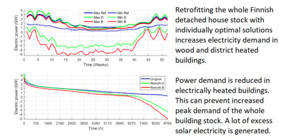
Air-to-air or ground-source heat pumps were utilized in all optimal retrofit solutions. Thus, some buildings will increase their electric power demands on the grid. Other studies have therefore assumed that new heat pumps cannot use the average low-emission electricity of the grid and would instead need to utilize the marginal production that is typically high emission coal generation [25]. However, the issue can be bypassed if the existing loads are lowered at the same time as new ones are added. This was the case in this study on the building stock level. New heat pumps increased electricity demand in the retrofitted wood heated or district heated buildings, but this was offset by the same solutions (heat pumps and envelope improvements) reducing electricity demand in the most power intensive buildings that were heated directly with electric radiators or electric boilers.

The optimization of retrofit solutions favored very large PV systems (4400 MW_p and 5600 MW_p) for the scenarios aiming for the largest emission reduction. However, the majority of the solar electricity generated by the oversized systems could not be used at the buildings and had to be exported to the grid. The maximum power levels of the exports were several times larger than the peak power demand in building without electric main heating systems. In those cases, the high-power requirement of the solar arrays could be a problem for the distribution grid, if it is not designed to handle such power. However, in electrically heated buildings the peak winter demand was on a similar level as the exports and the grid would presumably be able to handle the loads. However, a study on integration of variable renewables in the Finnish grid estimated that more than 1100 MW_p of solar electricity would decrease wind energy integration potential and significantly increase costs [39]. This shows the need for an additional study that looks at the building stock in more detail, while also including the effects of the national power grid and international transfers through the Nordic electricity market.

With the large amounts of excess solar energy going to the grid, the electricity spot price would likely drop. Solar electricity is produced in all buildings at the same time, so with enough excess power the price could go to zero or even to negative values. This would influence the LCC of the building retrofits, by lowering the lifetime value of solar electricity generation. Thus, if large scale retrofitting was done, the cost-optimal PV array size would go down. To avoid this, more ways to use the electricity are needed. Communities could use seasonal thermal energy storage to shift the use of electricity in summer to meet heating needs in winter. For example, solar electricity combined with borehole thermal energy storage for Finnish conditions was examined in [40]. Typically, demand response and short-term thermal energy storage in water tanks is also useful for increasing the value of solar electricity [41,42], but in the retrofit cases of the current study, solar thermal collectors were also included and handled most of the heating demand in summer. District heating could be produced with heat pumps [43]. Totally new uses for electricity are likely to appear. For example, the number of new electric car registrations in Finland has almost tripled in a year, though the absolute numbers are still low [44]. Other uses for excess electricity are in the energy intensive Finnish industry [45] or synthetic fuel production (also known as power-to-X) [46].

When GSHP was utilized, the annual peak electricity demand was significantly lower for the retrofit B cases than the original or retrofit D cases. This was due to higher heat pump thermal power capacity relative to the heating demand. When the heat pumps were sized to 60% or so of peak demand, electric backup heaters saw more use. Sizing the heat pump to above 90% made the peak electricity demand drop, also making the daily variance in demand smaller. This helps in sizing the electricity distribution infrastructure and designing energy storage systems. It is easier to optimize an energy storage system for power or energy capacity compared to having to maximize both.

The energy demand data for all the buildings were obtained through simulation. While dynamic simulation with IDA-ICE has been shown to be accurate, the results are sensitive to the background assumptions. Different age classes of single-family houses were modelled, but the shape and size of the basic building was the same for every case. The results could be different for smaller houses. In addition, only the southern climate zone of Finland was used for weather input data, creating a southern bias in the data. Further north, heating demand would be higher while solar energy generation would suffer. However, the majority of houses are located in the southern zone. Doing detailed calculations for two more climate zones would have tripled the number of cases and the need for time-consuming optimization. The results were obtained using the Test Reference Year 2012. Since building retrofitting is a long-term investment, climate change can influence the energy demand of the buildings during the lifetime of the buildings, as we move towards the year 2050. Cooling demand was ignored in this study, but it could be that as air-to-air heat pumps become more common, people will start using them for cooling as well, even though the heat pumps were purchased mainly for reducing heating expenses. This would increase the electric loads during summer, though this increase could mostly be mitigated by the increased amount of solar power.

The changes in the building stock were accounted for in a simplistic way, assuming all buildings are immediately retrofitted. In practice, many buildings in regions with declining populations and house values would likely not be retrofitted, due to the resident’s unwillingness to do long-term investments. A separate study is needed to calculate more feasible retrofit pathways, taking into account that change happens gradually and that new buildings are added while some old buildings are completely torn down. No flexibility or demand response methods were utilized, which removes the balancing element that appears when a large amount of buildings with different use profiles and energy storage systems are combined. In practice, on the building stock level, the peak power demand could thus be expected to be lower than in the cases presented in this study. The houses were assumed to be oriented south for solar energy purposes. In practice, some buildings are oriented badly, receive a lot of shading or are otherwise not suitable for solar energy installations. Thus, only a fraction of houses would be feasible for solar energy production.

There is uncertainty in the heating systems in use in the current building stock. Building owners do not always report changes to their heating system, such as when replacing an oil boiler with a heat pump. Some wood-heated buildings might actually use wood only as a backup energy source, while others use it as the main heat source. Thus, the real distribution of heating systems is not known. Possible changes to the electricity use of equipment and appliances in the buildings were not considered in the study. On the one hand, old appliances are gradually upgraded into more energy-efficient devices, which should reduce electricity consumption, but on the other hand, people are adding new electricity consuming equipment, which increases power demand. These trends could have an influence on the heating demand of buildings in the future through the excess heat they release.

5. Conclusions

Analyzing the hourly power demand of buildings helps in planning future generation capacity and backup and energy storage investments. The hourly heating and electric power demand of the Finnish detached house building stock was simulated using four different age categories of buildings, four different main heating systems and three levels of energy performance (reference, low cost retrofit D, and high impact retrofit B). Energy retrofits to improve energy efficiency had a significant effect on the peak and average power demand in all examined buildings. The main contribution of this paper was to show the power demand distribution before and after retrofits. Typically retrofit studies only show the effects of retrofits on the annual level, but this study presented the seasonal changes in power demand, to better understand what additional changes to the energy system are needed inside and outside the building sector. Another important contribution was the presented estimate of the net change in power demand in the building stock level if large-scale building energy retrofits are done.

The lower emissions of electricity compared to on-site boilers or district heating favor electrification of heating, through the use air-source heat pumps. This resulted in increased electricity demand in buildings with district heating or on-site wood boilers. At retrofit level B, the peak power demand of these building rose by 60 to 70%, but the absolute impact was low. On the other hand, buildings with direct electric heating significantly lowered their demand through the retrofits (peak demand down by 27 to 40% in retrofit B), as did buildings with ground-source heat pumps (peak demand down by 36 to 68%), with significant absolute impact.

These effects were combined in scenarios where all single-family houses of the whole building stock were retrofitted, which resulted in a net decrease in annual electricity use, −11% for low cost retrofits (scenario D), and −38% for high impact retrofits (scenario B). On the building stock level, peak power demand increased by 19% for low cost retrofits, but remained unchanged for the combined high impact retrofits. However, it is not likely that all buildings could be retrofitted in the same way in practice, due to both social and technical issues related to different conditions in each building.

The optimal solar electricity generation capacity on the individual building level was high. When the individual optima were utilized in the whole building stock, the peak excess power of solar electricity was 3.5 GW for the low cost retrofit scenario and 5 GW for the high impact retrofit. Such high values for unnecessary power generation could be difficult for the grid to handle. Such a scenario is also sensitive to price assumptions and might not be feasible if increasing excess production were to reduce solar energy value. This calls for further research on the optimization of individual building retrofits together with the power system as a whole. Future studies need to combine the changes in buildings and conventional power sector, as well as include new potential ways to use the available renewable energy. Seasonal thermal energy storage could be one way to solve the problem of overproduction, along with electric cars and power-to-X technologies.

Retrofitting old detached houses in Finland can reduce emissions significantly by improving thermal insulation values and by utilizing electrified heating with air-source or ground-source heat pumps. Fears of increasing the marginal electricity demand seem to be unfounded. While the amount of heat pumps is increased, reducing the energy demand in buildings with direct electric heating can prevent both the total electricity demand and peak power demand from rising at the building stock level. This bodes well for major retrofit projects based on electrification of the heating market. However, more accurate modelling of the building stock is needed. A future study should consider how the Finnish building stock could realistically be retrofitted, taking into account both the addition and removal of buildings as well as regional trends in population and economic activity.

References

1. European Commission. EU Climate Action-2050 Long-Term Strategy. 2016. Available online: https://ec.europa.eu/clima/policies/strategies/2050_en (accessed on 4 January 2020).
2. Kavvadias, K.; Jiménez-Navarro, J.P.; Thomassen, G. Decarbonising the EU Heating Sector - Integration of the Power and Heating Sector. Publications Office of the European Union, EUR 29772 EN. 2019. Available online: https://publications.jrc.ec.europa.eu/repository/bitstream/JRC114758/kjna29772enn.pdf (accessed on 7 February 2020).
3. European Parliament. Directive 2010/31/EU of the European Parliament and of the Council of 19 May 2010 on the Energy Performance of Buildings; European Parliament: Brussels, Belgium, 2010. [Google Scholar]
4. European Parliament. Directive (EU) 2018/844 of the European Parliament and of the Council Amending Directive 2010/31/EU on the Energy Performance of Buildings and Directive 2012/27/EU on the Energy Efficiency; European Parliament: Brussels, Belgium, 2018. [Google Scholar]
5. Ministry of the Environment. 4/13 Asetus Rakennuksen Energiatehokkuuden Parantamisesta Korjaus-ja Muutostöissä (4/13 Decree on Improving Energy Performance in Renovations). 2013. Available online: http://www.ym.fi/download/noname/%7B924394EF-BED0-42F2-9AD2-5BE3036A6EAD%7D/31396 (accessed on 17 January 2020).
6. Statistics Finland. Number of Buildings by Intended Use and Year of Construction on 31 Dec. 2015. 2016. Available online: http://pxnet2.stat.fi/PXWeb/pxweb/en/StatFin/StatFin__asu__rakke/?tablelist=true (accessed on 10 November 2019).
7. Oberegger, U.F.; Pernetti, R.; Lollini, R.; Ulrich, F.O.; Roberta, P.; Roberto, L. Bottom-up building stock retrofit based on levelized cost of saved energy. Energy Build. 2020, 210, 109757. [Google Scholar] [CrossRef]
8. Ekström, T.; Blomsterberg, Å. Renovation of Swedish Single-family Houses to Passive House Standard–Analyses of Energy Savings Potential. Energy Procedia 2016, 96, 134–145. [Google Scholar] [CrossRef] [Green Version]
9. Moran, P.; O’Connell, J.; Goggins, J. Sustainable energy efficiency retrofits as residenial buildings move towards nearly zero energy building (NZEB) standards. Energy Build. 2020, 211, 109816. [Google Scholar] [CrossRef]
10. Niemelä, T.; Kosonen, R.; Jokisalo, J. Cost-effectiveness of energy performance renovation measures in Finnish brick apartment buildings. Energy Build. 2017, 137, 60–75. [Google Scholar] [CrossRef] [Green Version]
11. Hirvonen, J.; Jokisalo, J.; Heljo, V.J.; Kosonen, R. Towards the EU emissions targets of 2050: Optimal energy renovation measures of Finnish apartment buildings. Int. J. Sustain. Energy 2018, 38, 649–672. [Google Scholar] [CrossRef] [Green Version]
12. Niemelä, T.; Levy, K.; Kosonen, R.; Jokisalo, J. Cost-optimal renovation solutions to maximize environmental performance, indoor thermal conditions and productivity of office buildings in cold climate. Sustain. Cities Soc. 2017, 32, 417–434. [Google Scholar] [CrossRef] [Green Version]
13. Hirvonen, J.; Jokisalo, J.; Heljo, J.; Kosonen, R. Towards the EU Emission Targets of 2050: Cost-Effective Emission Reduction in Finnish Detached Houses. Energies 2019, 12, 4395. [Google Scholar] [CrossRef] [Green Version]
14. Paiho, S.; Pulakka, S.; Knuuti, A. Life-cycle cost analyses of heat pump concepts for Finnish new nearly zero energy residential buildings. Energy Build. 2017, 150, 396–402. [Google Scholar] [CrossRef]
15. Grimm, V.; Zoettl, G. Investment Incentives and Electricity Spot Market Competition. J. Econ. Manag. Strat. 2013, 22, 832–851. [Google Scholar] [CrossRef] [Green Version]
16. Grimm, V.; Martin, A.; Schmidt, M.; Weibelzahl, M.; Zöttl, G. Transmission and generation investment in electricity markets: The effects of market splitting and network fee regimes. Eur. J. Oper. Res. 2016, 254, 493–509. [Google Scholar] [CrossRef] [Green Version]
17. Chen, Y.; Peng, X.; Gu, J.; Schmidt, F.P.; Li, W. Measures to improve energy demand flexibility in buildings for demand response (DR): A review. Energy Build. 2018, 177, 125–139. [Google Scholar] [CrossRef]
18. Xu, L.; Wang, S.; Xiao, F. An adaptive optimal monthly peak building demand limiting strategy considering load uncertainty. Appl. Energy 2019, 253, 113582. [Google Scholar] [CrossRef]
19. Deng, X.; Lv, T. Power system planning with increasing variable renewable energy: A review of optimization models. J. Clean. Prod. 2020, 246, 118962. [Google Scholar] [CrossRef]
20. Qu, K.; Chen, X.; Ekambaram, A.; Cui, Y.; Gan, G.; Økland, A.; Riffat, S. A novel holistic EPC related retrofit approach for residential apartment building renovation in Norway. Sustain. Cities Soc. 2020, 54, 101975. [Google Scholar] [CrossRef]
21. Garriga, S.M.; Dabbagh, M.; Krarti, M. Optimal carbon-neutral retrofit of residential communities in Barcelona, Spain. Energy Build. 2020, 208, 109651. [Google Scholar] [CrossRef]
22. Rakhshan, K.; Friess, W.A. Effectiveness and viability of residential building energy retrofits in Dubai. J. Build. Eng. 2017, 13, 116–126. [Google Scholar] [CrossRef]
23. Hirvonen, J.; Jokisalo, J.; Heljo, V.J.; Kosonen, R. Effect of apartment building energy renovation on hourly power demand. Int. J. Sustain. Energy 2019, 38, 918–936. [Google Scholar] [CrossRef]
24. Patronen, J.; Kaura, E.; Torvestad, C. Nordic Heating and Cooling; Nordic Council of Ministers: Copenhagen, Denmark, 2017. [Google Scholar]
25. Dodoo, A. Techno-economic and environmental performances of heating systems for single-family code-compliant and passive houses. E3S Web Conf. 2019, 111, 03039. [Google Scholar] [CrossRef] [Green Version]
26. EQUA Simulation. IDA ICE-Simulation Software. 2019. Available online: https://www.equa.se/en/ida-ice (accessed on 8 August 2019).
27. EQUA Simulation. Validation of IDA Indoor Climate and Energy 4.0 with Respect to CEN Standards EN 15255-2007 and EN 15265-2007; EQUA Simulation: Solna, Sweden, 2010. [Google Scholar]
28. Loutzenhiser, P.; Manz, H.; Maxwell, G. Empirical Validations of Shading/Daylighting/Load Interactions in Building Energy Simulation Tools; IEA-International Energy Agency: Zürich, Switzerland, 2007. [Google Scholar]
29. Koivuniemi, J. Lämpimän käyttöveden mitoitusvirtaama ja lämpötilakriteerit veden mikrobiologisen laadun kannalta kaukolämmitetyissä Taloissa Domestic Hot Water Design Flow and Temperature Criteria as Pertains to Water Microbiological Quality in District Heated Houses. In Finnish. M.Sc. Thesis, Helsinki University of Technology, Espoo, Finland, 2005. [Google Scholar]
30. Degefa, M.Z. Electrical Load Disaggregation-A Project Report of SGEM; SGEM: Espoo, Finland, 2012. [Google Scholar]
31. Palonen, M.; Hamdy, M.; Hasan, A. MOBO a new software for multi-objective building performance optimization. Presented at the 13th Conference of International Building Performance Simulation Association, Chambéry, France, 26–28 August 2013. [Google Scholar]
32. Deb, K.; Pratap, A.; Agarwal, S.; Meayarivan, T. A fast and elitist multiobjective genetic algorithm: NSGA-II. IEEE Trans. Evol. Comput. 2002, 6, 182–197. [Google Scholar] [CrossRef] [Green Version]
33. Saari, A.; Airaksinen, M. Energiatehokkuutta Koskevien vähimmäisvaatimusten Kustannusoptimaalisten Tasojen Laskenta; [In Finnish]; EU Commission: Brussels, Belgium, 2012; Available online: https://docplayer.fi/388965-Energiatehokkuutta-koskevien-vahimmaisvaatimusten-kustannusoptimaalisten-tasojen-laskenta-suomi.html (accessed on 7 April 2020).
34. Ministry of the Environment. Directive on Building Energy Certificates, Attachment 1 [In Finnish]. 2017. Available online: https://www.finlex.fi/data/sdliite/liite/6822.pdf (accessed on 12 December 2018).
35. Ministry of the Environment. Ympäristöministeriön asetus uuden rakennuksen energiatehokkuudesta (1010/2017) (Decree of the Ministry of the Environment on the Energy Performance of the New Building (1010/2017) [In Finnish]. 2018. Available online: https://www.finlex.fi/fi/laki/alkup/2017/20171010 (accessed on 12 January 2020).
36. Kalamees, T.; Jylhä, K.; Tietäväinen, H.; Jokisalo, J.; Ilomets, S.; Hyvönen, R.; Saku, S. Development of weighting factors for climate variables for selecting the energy reference year according to the EN ISO 15927-4 standard. Energy Build. 2012, 47, 53–60. [Google Scholar] [CrossRef]
37. Finnish Meteorological Institute. Test Reference Years for Energy Calculations [In Finnish]. 19 November 2018. Available online: https://ilmatieteenlaitos.fi/energialaskennan-testivuodet-nyky (accessed on 2 April 2019).
38. Finnish Energy. Aurinkosähkön tuotantokapasiteetti lisääntyi 82% vuodessa. Energiavirasto. Available online: https://energiavirasto.fi/tiedote/-/asset_publisher/aurinkosahkon-tuotantokapasiteetti-lisaantyi-82-vuodessa (accessed on 13 February 2020).
39. Zakeri, B.; Syri, S.; Rinne, S. Higher renewable energy integration into the existing energy system of Finland–Is there any maximum limit? Energy 2015, 92, 244–259. [Google Scholar] [CrossRef]
40. Hirvonen, J.; Sirén, K. A novel fully electrified solar heating system with a high renewable fraction—Optimal designs for a high latitude community. Renew. Energy 2018, 127, 298–309. [Google Scholar] [CrossRef]
41. Hirvonen, J.; Kayo, G.; Hasan, A.; Sirén, K. Zero energy level and economic potential of small-scale building-integrated PV with different heating systems in Nordic conditions. Appl. Energy 2016, 167, 255–269. [Google Scholar] [CrossRef]
42. Schibuola, L.; Scarpa, M.; Tambani, C. Demand response management by means of heat pumps controlled via real time pricing. Energy Build. 2015, 90, 15–28. [Google Scholar] [CrossRef]
43. Arabkoohsar, A.; AlSagri, A.S. A new generation of district heating system with neighborhood-scale heat pumps and advanced pipes, a solution for future renewable-based energy systems. Energy 2020, 193, 116781. [Google Scholar] [CrossRef]
44. Traficom, Uusien henkilöautojen ensirekisteröinnit laskussa–sähköautojen ja käytettyjen ladattavien hybridien määrät kasvussa, Traficom. Available online: https://www.traficom.fi//fi/ajankohtaista/uusien-henkiloautojen-ensirekisteroinnit-laskussa-sahkoautojen-ja-kaytettyjen (accessed on 13 February 2020).
45. Rehfeldt, M.; Worrell, E.; Eichhammer, W.; Fleiter, T. A review of the emission reduction potential of fuel switch towards biomass and electricity in European basic materials industry until 2030. Renew. Sustain. Energy Rev. 2020, 120, 109672. [Google Scholar] [CrossRef]
46. Hänggi, S.; Elbert, P.; Bütler, T.; Cabalzar, U.; Teske, S.; Bach, C.; Onder, C. A review of synthetic fuels for passenger vehicles. Energy Rep. 2019, 5, 555–569. [Google Scholar] [CrossRef]
Figure 1. The process chart for the utilized simulation and optimization method.
Energies 13 01773 g001
Figure 2. Distribution of main heating systems in the building stock within each building age category.
Energies 13 01773 g002
Figure 3. Top: The ventilation and heat distribution systems for the reference buildings. Bottom: The retrofit paths considered.
Energies 13 01773 g003
Figure 4. District heating use of all district heated houses. On the left: The hourly duration curve of district heating (DH) power demand for the whole year. On the right: The sustained peak/bottom DH power demand. Solid lines depict the weekly top 5% of demand and dotted lines the weekly bottom 5% of demand.
Energies 13 01773 g004
Figure 5. Electric power demand of the district heated buildings. Negative values represent exports of excess electricity back to the grid. On the left: The hourly duration curve of power demand for the whole year. On the right: Sustained peak/bottom power demand. Solid lines depict the weekly top 5% of demand and dotted lines the weekly bottom 5% of demand.
Energies 13 01773 g005
Figure 6. Electric power demand of the wood-heated buildings. Negative values represent exports of excess electricity back Table 5 of demand, and dotted lines depict the weekly bottom 5% of demand.
Energies 13 01773 g006
Figure 7. Electric power demand of the buildings with direct electric heating. Negative values represent exports of excess electricity back to the grid. On the left: The hourly duration curve of power demand for the whole year. On the right: the sustained peak/bottom power demand. Solid lines depict the weekly top 5% of demand, and dotted lines depict the weekly bottom 5% of demand.
Energies 13 01773 g007
Figure 8. Electric power demand of the buildings with ground-source heat pumps. Negative values represent exports of excess electricity back to the grid. On the left: The hourly duration curve of power demand for the whole year. On the right: Sustained peak/bottom power demand. Solid lines depict the weekly top 5% of demand, and dotted lines depict the weekly bottom 5% of demand.
Energies 13 01773 g008
Figure 9. Annual electricity demand for the whole detached house stock. Also shown is the excess solar electricity produced in the buildings. Usable solar is surplus production from some detached houses that could be used in other houses, while Excess solar is surplus that needs to be used in some other sector (values presented).
Energies 13 01773 g009
Figure 10. Sustained peak and bottom electric power (5% of weekly hours) in the whole building stock with the original systems and in the retrofit scenarios D and B. Also shown are the hourly duration curves of the same original data.
Energies 13 01773 g010