Multi-Time Scale Optimization Scheduling Strategy for Combined Heat and Power System Based on Scenario Method

Abstract

The wind–heat conflict and wind power uncertainty are the main factors leading to the phenomenon of wind curtailment during the heating period in the northern region of China. In this paper, a multi-time scale optimal scheduling strategy for combined heat and power system is proposed. Considering the temporal dependence of wind power fluctuation, the intra-day wind power scenario generation method is put forward, and both day-ahead and intra-day optimization scheduling models based on the scenario method are established to maximize the system’s revenue. The case analyzes the impacts of the initial heat storage capacity of a heat storage device and different scheduling strategies on system revenue. It is verified that the scheduling strategy can better adapt to wind power uncertainty and improve the absorption capacity of wind power, while ensuring the safety and economical efficiency of system operation.

1. Introduction

At present, wind power (WP) is developing rapidly all over the world. By the end of June 2019, the cumulative installed capacity of wind power in China reached 193 million kW, of which 9.09 million kW was newly installed from January to June 2019. However, in the rapid development of wind power, the problem of wind power accommodation is particularly prominent. According to the National Energy Administration of China, the national average wind power utilization hours in the first half of 2019 were 1133 hours, and wind power curtailment reached 10.5 billion kW·h in the first six months [1].

The main reason for wind curtailment is the uncertainty of wind power output [2], which requires more flexible adjustment resources than conventional units. However, in the northern region of China, where wind power resources are abundant, flexible power sources such as pumped storage station and gas station account for less than 4% of the total. Peak regulation in winter is particularly difficult. In addition, due to the superposition of “three phases” during the heating period, through the period of electricity consumption and peak period of wind power generation, most of the wind energy is curtailed in the late night of the winter heating period. Furthermore, the thermal-electric coupling of the combined heat and power (CHP) unit limits the electric power regulating ability and intensifies the wind curtailment phenomenon.

In order to reduce the wind curtailment in the winter heating period, a large number of studies have been conducted to improve the regulating capacity of CHP units [3]. The authors of [4] analyzed the operating characteristics of the CHP unit configured with heat storage and the peak shaving ability, and a dispatching model for combined heat and power system (CHPS) with heat storage device (HSD) was established, which verified the effectiveness of the model for improving wind power accommodation. In [5], two aspects of scheduling model and optimization control were discussed, and the specific implementation of heat storage in CHP units to improve the system’s ability to absorb wind power was studied. The authors of [6] presented a model that determined the theoretical maximum of flexibility of a combined heat and power system (CHPS) coupled to a thermal energy storage solution that can be either centralized or decentralized. The authors of [7] presented the issue of robust operation of a multicarrier energy system with electric vehicles and CHP units. However, these above studies did not consider the impact of wind power uncertainty on the scheduling results, and only the operation mode under the typical daily wind power output curve is considered. Therefore, the authors of [8] considered the randomness of wind power output, and the stochastic optimization dispatching model based on scenario method was established, and solved the uncertainty problem of wind power output well. In [9], to cope with the uncertainties of the renewable energy sources and loads, some scenarios were generated using the scenario-based analysis. Nevertheless, the prediction accuracy of wind power output is not high enough, and the forecasting error of wind power is positively correlated with time. The result in single day-ahead scheduling plan differs greatly from the day’s operating output, and cannot be applied to the CHPS with large-scale wind power. In view of this, the authors of [10] established the intra-day rolling scheduling model and adopted the intra-day rolling scheduling to modify the day-ahead plan output. In [11], through day-ahead scheduling, day-in rolling, and real-time dispatch, the influence of uncertain factors on microgrid cluster’s stable and economic operation could be eliminated to the most extent; whereas, in the above literatures, the impact of initial heat storage capacity of the HSD on the optimization results was not discussed, and most of them assigned a fixed value such as the total or half capacity of the HSD. Furthermore, the operation optimization of HSD is a typical multi-stage decision problem, with close relationship between different periods, but the intra-day scheduling plan cannot be globally optimized because it is a phased plan (four hours), whereas the wind power uncertainty model used in most of the current researches did not consider the temporal dependence of wind power fluctuation.

Based on problems above, a multi-time scale optimal scheduling strategy based on scenario method in this paper is proposed for the CHPS including WP unit, thermal power (TP) unit, and CHP unit with HSD. First, based on short-term wind power forecast data, the day-ahead optimization scheduling model based on the scenario method is established to maximize the benefit of CHPS. The optimal initial heat storage capacity of the HSD is determined by analyzing the impact on the overall revenue of the system. At this time, the day-ahead scheduling plan is obtained. Then, based on the day-ahead scheduling plan and the ultra-short-term prediction data of wind power, considering the temporal dependence of wind power fluctuation, the intra-day wind power scenario generation method is put forward. Moreover, the intra-day rolling scheduling model is also established to maximize the benefit of CHPS, and solved by using commercial optimization software Cplex, which is provided by IBM (International Business Machines Corporation) in Armonk, NY, USA. The expected values of the decision variables in dispatch period are used as the intra-day plan to adjust and modify the previous plan. Finally, the value of each decision variable at this moment is taken as the boundary condition of the next rolling scheduling period, and the above steps are cycled until the end of the whole day-ahead scheduling plan. The simulation is compared with the dispatch model that does not consider this, and the effectiveness to improve system revenue and promote wind power consumption is verified.

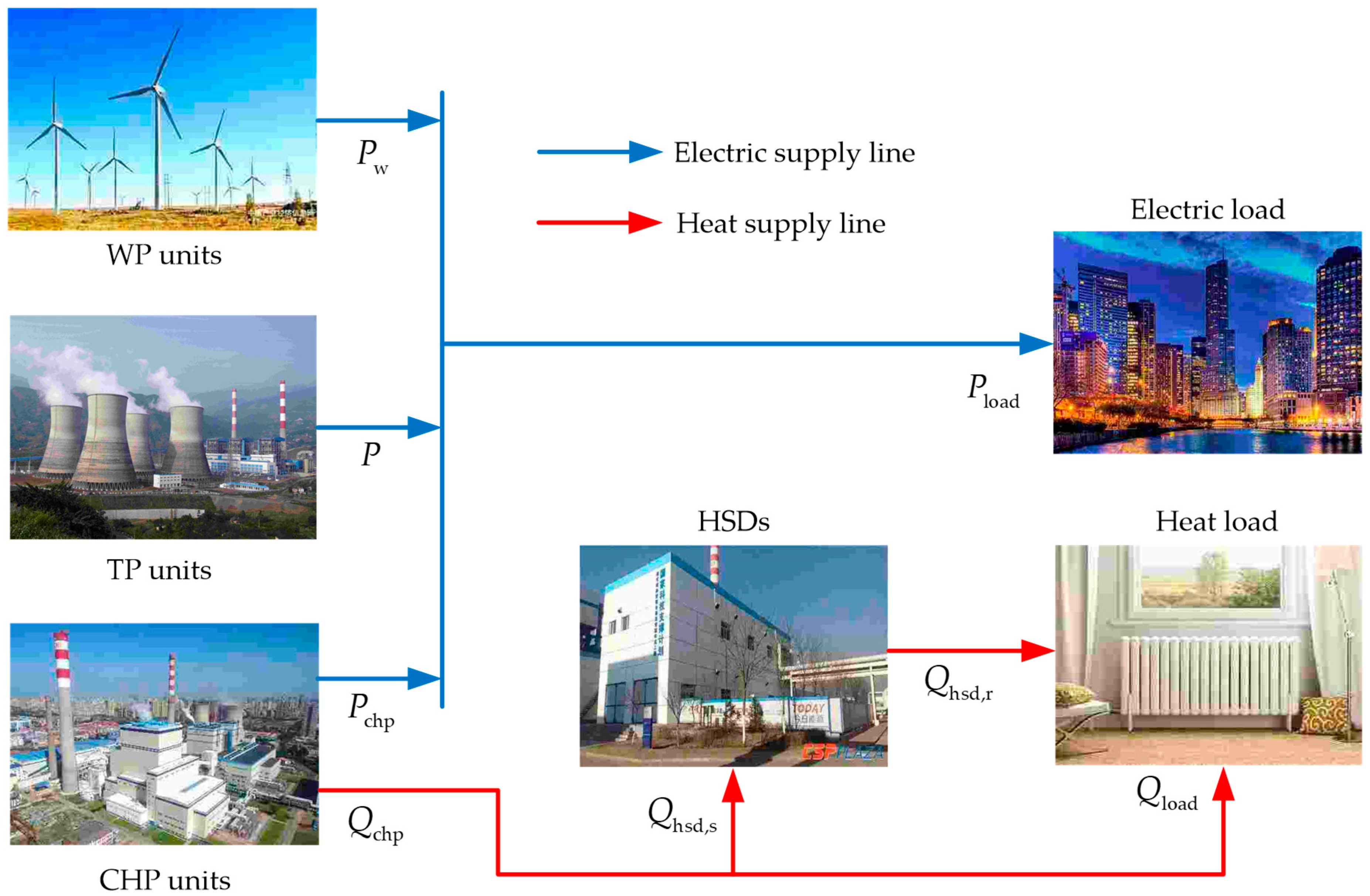
The paper is structured as follows. In Section 2, the structure of the CHPS is described. The day-ahead optimal scheduling model is established in Section 3. The intra-day rolling optimization scheduling model is proposed in Section 4. The model’s solution method is described in detail in Section 5, and the case study is presented in Section 6. Finally, the conclusions are drawn in Section 7.

2. Structure of the Combined Heat and Power System

The brief structure of the CHPS including the TP units and the WP units, as well as the CHP units with HSDs, is shown in Figure 1.

By adding the HSD, the CHPS can break the rigid constraint of the CHP unit and increase the regulating capacity. Traditional CHP units are generally constrained by “power determined by heat” during the winter heating period. With the addition of the HSD, the heat output of the CHP unit will not have to be balanced with the heat load in real time by controlling the heat storage and heat release of the HSD. In this way, the CHP unit will break the rigid constraint of “power determined by heat” and can have certain flexibility of regulation, to enhance the system’s regulation capacity and the accommodation of wind power.

3. Day-ahead Optimization Scheduling Model

3.1. Objective Function

The day-ahead optimal scheduling model of CHPS takes the highest expected value of the system operating revenue under different wind power output scenarios as the objective function [12], which is composed of the power and heat supply benefits minus the operation cost of the units and penalty cost in the system. In order to encourage the system to accommodate more wind power, the cost of wind power generation is ignored.

$$\max f_1={\displaystyle \sum _{k=1}^{N_k}{\rho }_k{\displaystyle \sum _{t=1}^T(S_t^k-C_t^k-C_{\mathrm{pun},t}^k)}}$$

(1)

where $k$ is scenario numbering. $N_k$ is the total number of scenarios. ${\rho }_k$ is the probability of scenario $k$. $T$ is the total scheduling time. $S_t^k$, $C_t^k$, and $C_{\mathrm{pun},t}^k$ are the power and heat supply benefits, the operation cost of the units, and the penalty cost at moment $t$ under scenario $k$, respectively.

In the CHPS, to encourage more wind power accommodation, the cost of wind power generation can be ignored. The system operating cost includes the cost of generating electricity from TP units, the cost of generating electricity, and heat from CHP units [13].

3.1.1. Generation Cost of TP Units

Due to the uncertainty of wind power, the peak-shaving tasks undertaken by (TP) units have been aggravated, and the operating status has also changed accordingly. The power generation cost of TP units in the dispatching model includes the start-up and shutdown cost and operating cost. As the start-up and shutdown of the unit are not considered in day-ahead dispatch, this paper only considers the operating cost of TP units.

$$F_1={\displaystyle \sum _{t=1}^T{\displaystyle \sum _{i=1}^N[a_i{(P_{i,t}^k)}^2+b_i{P}_{i,t}^k+c_i]}}$$

(2)

where $F_1$ is the operating cost of TP units. $a_i$, $b_i$, and $c_i$ are the second-order fitting coefficients of the operating cost of unit $i$. $N$ is the total number of TP units. $P_{i,t}^k$ is the electrical output of unit $i$ at moment $t$ under scenario $k$.

3.1.2. Generation Cost of CHP Units

The CHP units not only bear the electric output of the system, but also undertake the heating task. Therefore, these units are in continuous operation during the heating period, so the generation cost of CHP units only includes the operating cost too. After removing the heat supply of HSD at time $t$, the heat output can be converted into the electric output under the pure condensing condition and then calculated by Formula (3) [14].

$$F_2={\displaystyle \sum _{t=1}^T{\displaystyle \sum _{i=1}^C\{a_{\mathrm{c}i}{[P_{\mathrm{c}i,t}^k+C_v(Q_{\mathrm{c}i,t}^k+Q_{\mathrm{s}i,t}^k)]}^2+}}{b}_{\mathrm{c}i}[P_{\mathrm{c}i,t}^k+C_{\mathrm{v}}(Q_{\mathrm{c}i,t}^k+Q_{\mathrm{s}i,t}^k)]+c_{\mathrm{c}i}\}$$

(3)

where $F_2$ is the operating cost of CHP units. $a_{\mathrm{c}i}$, $b_{\mathrm{c}i}$, and $c_{\mathrm{c}i}$ are the second-order fitting coefficients of the operating cost of CHP unit $i$. $C$ is the total number of CHP units. $C_{\mathrm{v}}$ is the operating cost parameters of units. $P_{\mathrm{c}i,t}^k$ and $Q_{\mathrm{c}i,t}^k$ are the electrical output and heat output of unit $i$ at time $t$ under scenario $k$, respectively. $Q_{\mathrm{s}i,t}^k$ is the heat storage and release power (positive storage and negative discharge) of the HSD at time $t$ under scenario $k$.

3.1.3. Wind Curtailment and Load Shedding Penalty

The penalty cost mainly includes the load shedding penalty when the actual wind power output being less than the planned output [15], and the wind curtailment penalty when the wind power being greater than the planned output.

$$\{\begin{array}{l}{P}_{\mathrm{w}i,t}^{\mathrm{cut}}=P_{\mathrm{w}i,t}^{\max }-P_{\mathrm{w}i,t} , P_{\mathrm{w}i,t}^{\max }>P_{\mathrm{w}i,t} \\ P_{\mathrm{load},t}^{\mathrm{cut}}=P_{\mathrm{w}i,t}-P_{\mathrm{w}i,t}^{\max } , P_{\mathrm{w}i,t}^{\max }<P_{\mathrm{w}i,t} \end{array}$$

(4)

where $P_{\mathrm{w}i,t}^{\mathrm{cut}}$ and $P_{\mathrm{load},t}^{\mathrm{cut}}$ are the curtailed wind power and the load shedding power at moment $t$, respectively. $P_{\mathrm{w}i,t}$ is the wind power output scheduled at time $t$. $P_{\mathrm{w}i,t}^{\max }$ is the maximum wind power output at moment $t$ on the day of dispatch.

The total penalty cost can be expressed as

$$C_{\mathrm{pun}}^k={\displaystyle \sum _{t=1}^T(\gamma \times P_{\mathrm{w}i,t}^{\mathrm{cut},k}+\beta \times P_{\mathrm{load},t}^{\mathrm{cut},k})}$$

(5)

where $\gamma$ and $\beta$ are the penalties for unit curtailment of wind and load shedding, respectively. $P_{\mathrm{w}i,t}^{\mathrm{cut},k}$ and $P_{\mathrm{load},t}^{\mathrm{cut},k}$ are the curtailed wind power and load shedding power at moment $t$ under scenario $k$, respectively.

3.2. Constraints

The constraints of the day-ahead scheduling model include the operating constraints of each unit, the operating constraints of HSDs, the electric load and thermal load balance constraints, and network security constraints.

3.2.1. Operation Constraints of WP Units

In this paper, a discrete scenario set is used to describe the uncertainty of wind power output. It is assumed that the maximum predicted output of WP unit $i$ at time $t$ under scenario $k$ is $P_{\mathrm{w}i\max ,t}^k$, and the constraints in the day-ahead scheduling model are as follows,

$$0\le P_{\mathrm{w}i,t}^k\le P_{\mathrm{w}i\max ,t}^k$$

(6)

where $P_{\mathrm{w}i,t}^k$ is the wind power output at time $t$ under scenario $k$.

3.2.2. Operation Constraints of TP Units

The upper and lower limits of output constraints and the climb rate constraints of TP units are mainly considered in the day-ahead scheduling model. The specific constraints are as follows,

$$P_{i\min }^{}\le P_{i,t}^k\le P_{i\max }^{}$$

(7)

$$-R{D}_{i,\max }^{}\cdot \Delta t\le P_{i,t}^{}-P_{i,t-1}^{}\le R{U}_{i,\max }^{}\cdot \Delta t$$

(8)

where $P_{i\min }^{}$ and $P_{i\max }^{}$ are the limits of $P_{i,t}^k$. $-R{D}_{i,\max }^{}$ and $R{U}_{i,\max }^{}$ are the maximum climb rate of unit $i$. $\Delta t$ is the interval per unit time.

3.2.3. Operation Constraints of CHP Units

This paper considers the CHP unit type of extraction, which has a coupling constraint on the heat and electric output [16]. When the heat output is constant, the unit’s electric output is limited to a specific interval [8], as shown in Figure 2.

The output feasible range of the CHP unit can be expressed as

$$\{\begin{array}{l}0\le Q_{\mathrm{c}i,t}^k\le Q_{\mathrm{c}i,\max }\\ P_{\mathrm{c}i,t}^k\le p_1+k_1{Q}_{\mathrm{c}i,t}^k\\ P_{\mathrm{c}i,t}^k\ge p_2+k_2{Q}_{\mathrm{c}i,t}^k\\ P_{\mathrm{c}i,t}^k\le p_3+k_3(Q_{\mathrm{c}i,t}^k-Q_{\mathrm{m}})\end{array}$$

(9)

where $k_1$, $k_2$, and $k_3$ are the unit operation coefficients. $p_1$ and $p_2$ are the maximum and minimum values of generating power when the unit’s air extraction value is zero, respectively. $p_3$ is the minimum electrical power of the unit. $Q_{\mathrm{m}}$ is the heating power corresponding to the minimum electrical power of the unit. $Q_{\mathrm{c}i,\max }$ is the maximum heating power of unit $i$.

The output change of CHP unit is determined by the amount of air extraction. Therefore, its climbing rate should be converted to the electric power constraint under the unit’s pure condensing condition.

$$-R{D}_{ci,\max }^{}\cdot \Delta t\le {\overline{P}}_{\mathrm{c}i,t}^k-{\overline{P}}_{\mathrm{c}i,t-1}^k\le R{U}_{ci,\max }^{}\cdot \Delta t$$

(10)

where ${\overline{P}}_{\mathrm{c}i,t}^k$ is the electric power of unit $i$ converted to pure condensing condition at time $t$ under scenario $k$. $R{D}_{ci,\max }^{}$ and $R{U}_{ci,\max }^{}$ are the maximum climb rate of CHP unit $i$.

3.2.4. Operation Constraints of HSDs.

The operation constraints of HSDs mainly include heat storage and release power constraints, the thermal storage tank capacity constraints, state constraints, and the cycle constraints of HSD [13]. The specific constraint expression is as follows,

$$\{\begin{array}{l}-Q_{\mathrm{f}i,\max }^{}\le Q_{\mathrm{s}i,t}^k\le Q_{\mathrm{z}i,\max }^{}\\ 0\le S_{\mathrm{eh},t}^k\le S_{\mathrm{eh},\max }^{}\\ S_{\mathrm{eh},t}^k=S_{\mathrm{eh},t-1}^k+Q_{\mathrm{s}i,t}^k-{\phi }_{\mathrm{eh}}{S}_{\mathrm{eh},t-1}^k\\ {\displaystyle \sum _{t=1}^T{Q}_{\mathrm{s}i,t}^k}=0\end{array}$$

(11)

where $Q_{\mathrm{f}i,\max }^{}$ and $Q_{\mathrm{z}i,\max }^{}$ are the maximum heat release and storage power of HSDs, respectively. $S_{\mathrm{eh},\max }^{}$ is the maximum heat storage capacity of the thermal storage tank. ${\phi }_{\mathrm{eh}}$ is the heat loss rate, which is generally taken as 0.05.

3.2.5. Electric Load and Heat Load Balance Constraints

$$\{\begin{array}{l}{\displaystyle \sum _{i=1}^W{P}_{\mathrm{w}i,t}^k}+{\displaystyle \sum _{i=1}^N{P}_{i,t}^k}+{\displaystyle \sum _{i=1}^C{P}_{ci,t}^k}=P_{\mathrm{load},t}\\ {\displaystyle \sum _{i=1}^C(Q_{ci,t}^k-Q_{\mathrm{s}i,t}^k)}=Q_{\mathrm{load},t}\end{array}$$

(12)

where $P_{\mathrm{load},t}$ and $Q_{\mathrm{load},t}$ are the electricity and heat load requirements at time $t$ of the CHPS, respectively.

3.2.6. Network Security Constraints

$$P_{l,\min }^{}\le P_{l,t}^k\le P_{l,\max }$$

(13)

where $P_{l,t}^k$ is the power of line $l$ at time $t$ under scenario $k$. $P_{l,\min }^{}$ and $P_{l,\max }$ are the limits of $P_{l,t}^k$.

4. Intra-Day Rolling Optimization Scheduling Model

As the prediction error of wind power output is positively correlated with time [17], the intra-day rolling scheduling model of the CHPS utilizes the ultra-short-term forecast output of wind power to optimize and adjust the day-ahead scheduling plan to ensure the economical efficiency of the system. However, the operation optimization of HSD is a typical multi-stage decision problem, with close relationship in different periods, and the intra-day scheduling plan cannot be globally optimized because it is a phased plan.

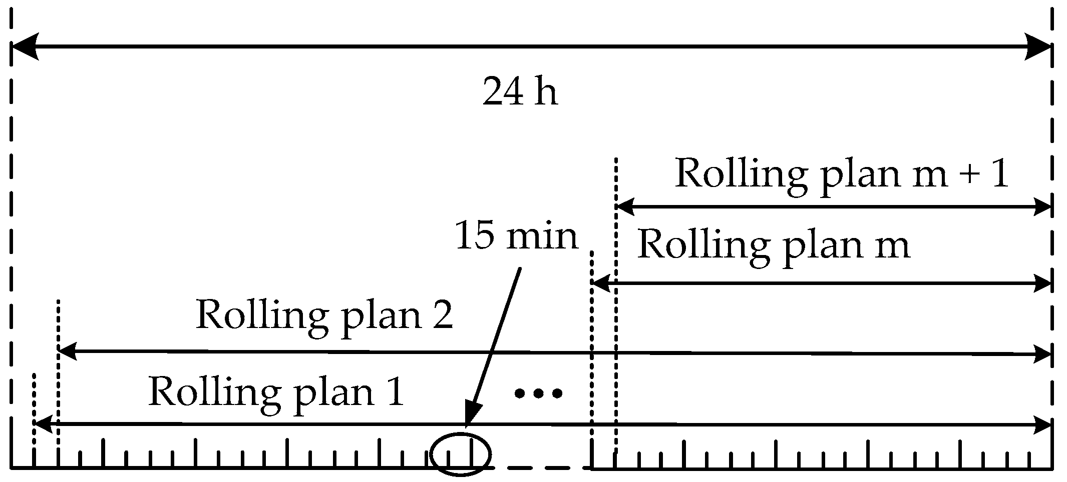
Based on the problem, the adapted intra-day rolling scheduling strategy is proposed in this paper, and it is shown in Figure 3. By adopting this scheduling strategy, it can ensure that the results of each rolling scheduling are the global optimal solutions.

As the scheduling time scale is changed, the data form of wind power input is also changed. In order to obtain the wind power input applicable to the scheduling strategy, this paper is based on the ultra-short-term prediction data of wind power, and considering the temporal dependence of wind power fluctuation, the intra-day wind power scenario generation method is put forward, and it is shown in Figure 4. First, the weighted Euclidean distance method is adopted to calculate the similarity to the corresponding period of the day-ahead scenario set of wind power, and the scenarios with the high similarity degree are extracted to form a new scenario set. Then, the ultra-short-term wind power prediction data is used to update the wind power output of the corresponding period of the new scenario set. Based on ultra-short-term electric and heat load forecast data, the intra-day rolling optimization scheduling model is solved to roll and modify the day-ahead scheduling plan. At last, the optimization result obtained at this time is taken as the boundary condition of the next rolling scheduling period, and the above steps are cycled until the end of the whole day-ahead scheduling plan.

4.1. Intra-Day Wind Power Scenario Generation

Euclidean distance represents the meaning of distance in the general sense, and is often used to measure the degree of similarity between two variables. The closer the distance is, the higher the similarity is between the two variables. The calculation method is as follows,

$$dis{t}_{ed}(x,y)={({\displaystyle \sum _{i=1}^n{(x_i-y_i)}^2})}^{\frac{1}{2}}$$

(14)

where $x$ and $y$ are the quantities. $n$ is the dimension of the vector.

Suppose $k=[P_{\mathrm{w},1}^k,P_{\mathrm{w},2}^k,\cdot \cdot \cdot ,P_{\mathrm{w},96}^k]\in K$ is a certain scenario data of wind power short-term forecast, and $s=[p_{t+1},p_{t+2},\cdot \cdot \cdot ,p_{t+16}]$ is the ultra-short-term forecast data obtained four hours in advance. Considering that the wind power output at time $t$ has time correlation characteristics with the previous time, and the longer the interval is, the weaker the correlation is; therefore, the weighted Euclidean distance is adopted to characterize this feature when calculating the similarity of two scenarios, and the wind power output change rate at the two moments is defined as

$$\Phi =\frac{|P_{w,t+1}-P_{w,t}|}{P_{w,t}}\times 100\%$$

(15)

calculate the change rates of $P_{w,t}$ with $P_{w,t-4},\cdot \cdot \cdot ,P_{w,t-1}$, respectively, and the sample proportion ${\tau }_i$ whose change rate within the range of 10% is also calculated. Then, the correlation weight coefficient ${\omega }_i$ at each moment is defined as

$${\omega }_i=\frac{{\tau }_i}{{\displaystyle \sum _{i=1}^{16}{\tau }_i}}$$

(16)

the Euclidean distance between $k\prime =[P_{\mathrm{w},t+1}^k,P_{\mathrm{w},t+2}^k,\cdot \cdot \cdot ,P_{\mathrm{w},t+16}^k]$ and $s$ is

$$dis{t}_{ed}(k\prime ,s)={({\displaystyle \sum _{i=1}^{16}{\omega }_i{(P_{\mathrm{w},t+i}^k-p_{t+i})}^2})}^{\frac{1}{2}}$$

(17)

then the scenario whose similarity meets certain requirements is selected:

$$\{\begin{array}{l}dis{t}_{ed}(k\prime ,s)\le \epsilon \\ {\rho }_{k\prime }={\rho }_k\end{array}$$

(18)

where $\epsilon$ is the maximum distance limit that satisfies the conditions. ${\rho }_{k\prime }$ is the probability of scenario $k\prime$.

Replacing the wind power output in the period of $t+1~t+16$ at scenario $k$ with $s$ is denoted as the new scenario $j$. The probability of the scenario $j$ is

$${\rho }_j=\frac{{\rho }_{k\prime }}{{\displaystyle \sum _{k\prime =1}^{N_j}{\rho }_{k\prime }}}$$

(19)

where $N_j$ is the number of screened scenarios.

In conclusion, the intra-day scenario set $J$ of wind power output during the day is obtained.

4.2. Objective Function

The objective function of the intra-day rolling dispatch model is still maximized by the system’s revenue, taking into account the power and heat supply benefits minus the operation cost of the units and penalty cost in the system, which is the same as in Equation (1).

4.3. Constraints

The constraints of the intra-day rolling scheduling model are roughly the same as those of the day-ahead scheduling model, and only the bias constraint is added to make the scheduling result better be connected with the day-ahead dispatch plan [10].

$$|P_{\mathrm{roll},t}^j-P_{\mathrm{day},t}^j|\le \zeta$$

(20)

where $P_{\mathrm{roll},t}^j$ and $P_{\mathrm{day},t}^j$ are the rolling plan and the day-ahead plan total power generation in time period $t$ under scenario $j$, respectively. $\zeta$ is the limit of power deviation.

In addition, the output and climb rate constraints of each unit, the operation constraints of HSDs, the electric load and heat load balance constraints, and network security constraints are considered, as shown in Equations (6)–(13).

5. Calculating Procedures

Simultaneous to Equations (1)–(13), the day-ahead optimization scheduling model of the CHPS is obtained. The random decision variables include the power output of each unit, the heat output of CHP units, and the heat storage and release power of HSDs. First, based on short-term wind power forecast data, a large number of wind power scenes are obtained. Then, the initial heat storage of the HSD is set to 0, and the model is solved by commercial optimization software Cplex, which is provided by IBM (International Business Machines Corporation) in Armonk, NY, USA [8]. Then, the initial heat storage capacity is iteratively modified to obtain the day-ahead scheduling plan set with different values. The value of the heat storage corresponding to the subset with the highest benefits is the optimal initial heat storage capacity of the HSD, and the expected value of each decision variable in the subset is the day-ahead scheduling plan of the system.

Simultaneous to Equations (1) and (6)–(20), the intra-day rolling optimization scheduling model of the CHPS is established, in which the decision variables are the same as the day-ahead scheduling model. Based on the ultra-short-term wind power forecast data, the method introduced in section 4.1 is used to generate a scenario set of wind power. Then, based on the ultra-short-term electricity and heat load forecast data, as the input of the model, the intra-day rolling optimization scheduling model is solved, and the expected values of the decision variables in dispatch period are used as the intra-day plan to adjust and modify the previous plan. Finally, the value of each decision variable at this moment is taken as the boundary condition of the next rolling scheduling period, and the above steps are cycled until the end of the whole day-ahead scheduling plan. The solution process is shown in Figure 5.

6. Case Study

6.1. General Situation of Simulation

Numerical simulations are conducted on a local grid in Liaoning province, including a wind farm, a CHP unit with HSD, and two TP units. The supply price of electric and heating is shown in

Table A2. The supply price of electric and heating.

Supply Price ¥/MW⋅h	Time/h
	0–7	8–10	11–15	16–18	19–21	22–24
electric	200	500	800	500	800	500
heating	450	450	450	450	450	450

of Appendix A, and the parameters of units are detailed in

Table A3. The parameters of units.

Power Source Type	Installed Capacity	Power Output/MW		Climb Rate/MW		Operating Parameters
		Min	Max	Down	Up	a	b	c
WP unit	1×450MW	0	450	0	450	-	-	-
TP unit	2×250MW	50	250	50	50	0.0037	12.98	36
CHP unit	1×250MW	40	210	50	50	0.0044	13.29	39
HSD	1×360MW⋅h	0	360	50	60	-	-	-

of Appendix A [18,19]. The wind power scene set data is shown in Figure 6 [20,21], different colored lines represent the output of the WP unit under different scenarios. The ultra-short-term forecast data of wind power, electric load, and heat load data in the system are shown in Figure 7.

6.2. Impact of Initial Heat Storage Capacity on Overall Revenue

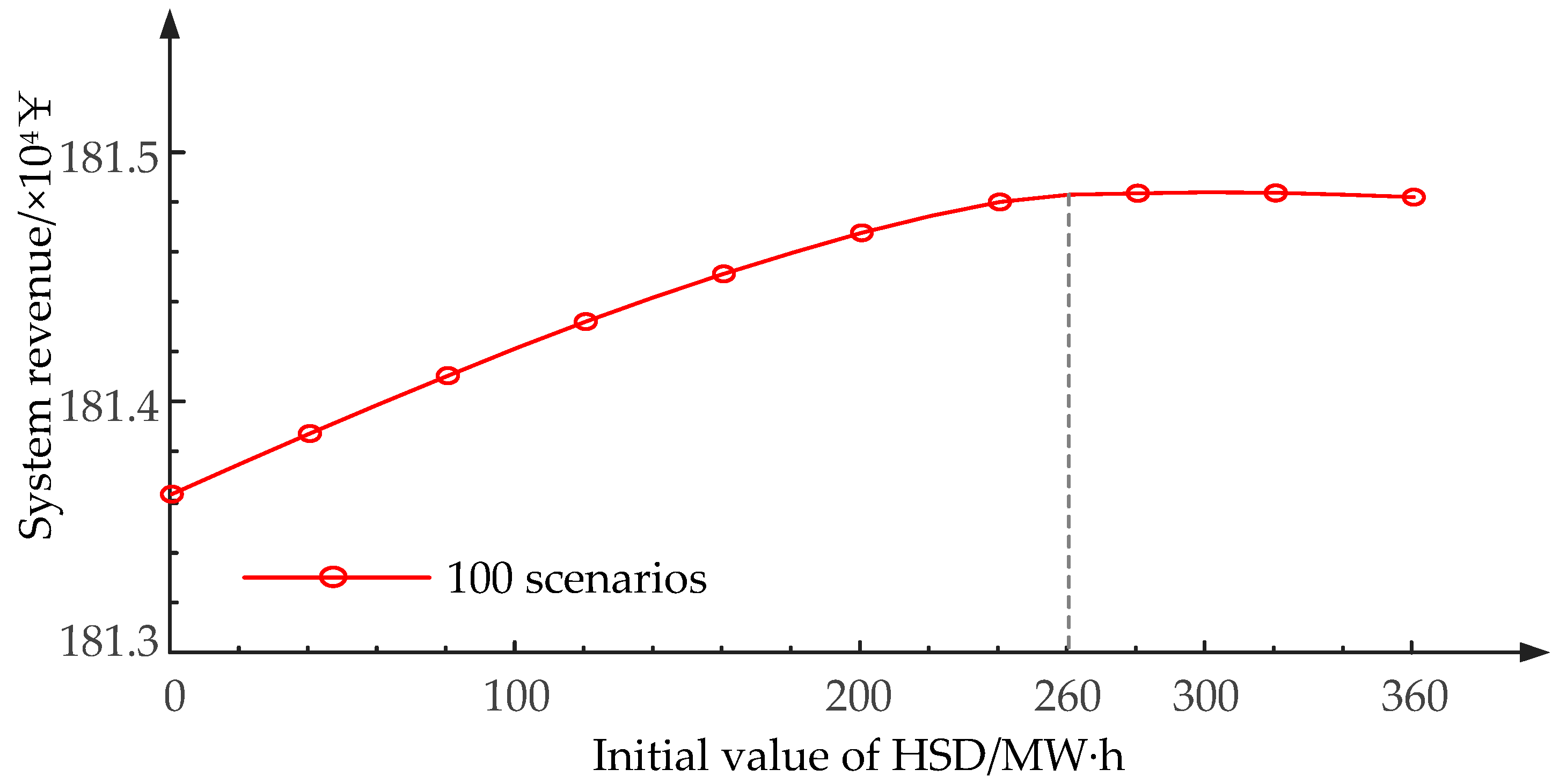
Before the day-ahead dispatch, a certain amount of heat needs to be stored in the HSD. In order to analyze the impact of initial heat storage capacity on the overall revenue of the system, the expected value of the overall revenue under different initial heat storage capacity is calculated. It can be seen from Figure 8 that both increase with the initial heat storage capacity, until the initial value of the heat storage reaches 260 MW⋅h and the system’s revenue is maximum. When the initial heat storage capacity is greater than 260 MW⋅h, the overall system revenue tends to be stable.

In order to analyze the effect of initial value on optimal scheduling results, two cases are considered:

Case 1: When the initial heat storage capacity is 0 MW⋅h.

Case 2: When the initial heat storage capacity is 260 MW⋅h.

Figure 9 shows the output of each unit of the system when the initial heat storage capacity is 0 MW⋅h and 260 MW⋅h. At this time, the expected revenue of the system is 1813.6 thousand yuan and 1814.7 thousand yuan, respectively. It can be seen from the figure that the wind power output of the wind farm is relatively large from 0 am to 7 am, and this is the period of low power load. If the initial heat storage capacity is low, the heat load demand can only be met by the CHP unit. However, the restriction of “determining power generation by heat” of the CHP unit will cause a large amount of wind power curtailment, and the inefficient use of renewable energy will lead to a decrease in revenue. When the initial heat storage capacity is 260 MW⋅h, from 0 am to 7 am, the heat load is jointly satisfied by the heat generation of the CHP unit and the HSD. At this time, the CHP unit is reduced electric output, so as to absorb more wind power to improve the total system revenue. When the initial heat storage capacity is greater than 260 MW⋅h, the overall system revenue tends to be stable. Therefore, considering the economics of the system, 260 MW⋅h is selected as the initial value of the HSD in the subsequent analysis and calculation.

6.3. Comparison of the Stochastic Model and Deterministic Model

In this part, two models are considered.

Case 3: Deterministic model.

The scheduling strategy of the deterministic model is based on the wind power output curve of the typical day to optimize and calculate the value of each decision variable. The objective function is as follows,

$$\max f_1={\displaystyle \sum _{t=1}^T(S_t^{}-C_t^{}-C_{\mathrm{pun},t}^{})}$$

(21)

Case 4: Stochastic model (established in this paper).

We assume that scenario 1 is the wind power output of the typical day, and output of each unit is calculated as the day-ahead scheduling plan of the deterministic model. Moreover, the day-ahead scheduling plan of the stochastic model is calculated by the method mentioned in the paper. Then, suppose that scenario 2 to scenario 100 are the actual wind power output on the dispatching day, the output of each unit under each scenario is obtained, and compared with the scheduling plan of the stochastic model and the deterministic model. The unit penalty cost for wind curtailment and load shedding is 100 yuan/MW⋅h, and the penalty cost in different scenarios is calculated. The results are shown in Figure 10.

It can be seen in Figure 10 that in more than 93% of the scenarios, the penalty cost of the scheduling plan calculated by the stochastic model is lower. Therefore, the scheduling plan arranged by the stochastic model can better adapt to the uncertainty of wind power.

6.4. Impact of Temporal Dependence of Wind Power Fluctuation on Overall Revenue

In this part, the two scheduling strategies are calculated separately.

Case 5: The traditional rolling scheduling strategy [22].

Case 6: The adapted rolling scheduling strategy.

The impact on the system revenue is analyzed, and the results under different scheduling strategies are shown in

Table 1. The system’s revenue before and after considering temporal dependence.

Items	Considering Temporal Dependence		Differential Values
	Before	After
Electric and heat income/×104¥	195.13	195.13	0
Costs of TP units/×104¥	7.07	7.02	0.05
Costs of CHP units/×104¥	6.01	5.94	0.07
Consumption of Wind Power/MW⋅h	5875.0	5941.4	66.4
Costs of Wind Curtailment penalty/×104¥	3.06	2.40	0.66
Total system‘s revenue/×104¥	178.99	179.77	0.78

.

When the temporal dependence is not considered, the cost of generating electricity for TP units and CHP units are 70,700 yuan and 60,100 yuan, which is an increase of 1200 yuan compared with the method of considering it. At the same time, after considering the temporal dependence, 66.4 MW⋅h of wind power is absorbed in the system, and the total revenue of the system increased by 7800 yuan than before.

Comparing Table 1 with Figure 11 and Figure 12, it can be seen that when the temporal dependence is not considered, the scheduling plan in each cycle (four hours) only needs to meet the highest return during this period. Therefore, at time 8–15, the electric load is high, but the wind power output is relatively small. In order to ensure the maximum stage benefits, the thermal output of the system is so small that HSD has no excess heat storage. At times 16–17 and 22–24, the wind power output is large, and the increased heat output of the CHP unit must not only meet the needs of the heat load, but also take into account the cycle constraints of the HSD, which shrinks the space for wind power accommodation. After considering temporal dependence, the HSD stores heat at 8–15 pm. When the subsequent wind power output is large, the heat storage device cooperates with the CHP unit to meet the heat load demand, thereby reducing the power output of the CHP unit. At the same time, more wind power is accommodated, and higher system revenue is obtained.

Furthermore, in order to consider the impact of potential uncertainty on the system, the system revenue and the additional wind power consumption under the two strategies with different times of wind power are studied, and the results are shown in Figure 13.

As can be seen from Figure 13, with increasing wind power output, the system revenue also increases. When the wind power is 1.3 times of the original data, the system revenue difference under the two scheduling strategies reaches the maximum. When wind power is 1.4 times the original data, the wind power consumption of system under the adapted scheduling strategy approaches the peak value first, so the system revenue is almost stable with increasing of wind power. When the wind power is 1.9 times the original data, both reach the maximum wind power consumption of the system under the two scheduling strategies. It can be seen that when considering wind power fluctuation, the adapted scheduling strategy can quickly approach the maximum wind power consumption level, so it is more suitable for the system with wind power fluctuation scenarios.

6.5. Algorithm Analysis

In this paper, the primal dual interior point method optimization program is used from the Cplex optimization toolbox. The interior point method is essentially a combination of the Lagrange function method, Newton method, and logarithmic barrier function method. It starts from the initial interior point and follows the steepest descent direction, moving directly from the inside of the feasible region to the optimal solution. Its salient feature is that the number of iterations has little relation to the system size. In the paper, the decision variables need to be optimized for each wind power output scenario, and the required accuracy can be achieved within 20 iterations. In the case of the intra-day rolling optimization dispatch process, a total of 15 iterations were performed. Changing of the objective function versus the number of iterations is shown in Figure 14.

7. Conclusions

Aiming at the problem of scheduling difficulties caused by the uncertainty and fluctuation of wind power output, this paper proposes a multi-time scale optimal scheduling strategy for CHPS based on the scenario method. Both day-ahead and intra-day optimization scheduling models are established to maximize the system’s revenue. The case analyzes the impacts of initial heat storage capacity of heat storage device and different scheduling strategies on system revenue. The main conclusions are as follows.

• The initial heat storage capacity of the HSD can affect the overall revenue of the system, which increases with the initial value. When the value is 260 MW⋅h, the system achieves the highest yield, so 260 MW⋅h is used as the optimal initial heat storage capacity of the HSD for subsequent analysis.
• In the day-ahead scheduling plan, compared with the deterministic model, it is verified that the day-ahead optimal scheduling model based on the scenario method can greatly reduce the system penalty cost, improve system benefits, and better adapt to the uncertainty of wind power.
• Compared with the scheduling method without considering the temporal dependence of wind power fluctuation, the results show that considering temporal dependence can better reserve more wind power absorption space for the system, promote the accommodation of wind power, and further improve the overall revenue of the system.

References

1. China’s Wind Power Grid Integration in the First Half of 2019. Available online: www.nea.gov.cn/2019-07/26/c_138259422.htm (accessed on 26 June 2019).
2. Xue, Y.S.; Lei, X.; Xue, F.; Yu, C.; Dong, C.Y.; Wen, F.S.; Jv, P. A review on impacts of wind power uncertainties on power systems. Proc. CSEE 2014, 34, 5029–5040. [Google Scholar] [CrossRef]
3. Hu, K.; Chen, Q. Overall energy efficiency and flexibility retrofit scheme analysis of heat-power integrated energy system. Therm. Power Gener. 2018, 47, 14–21. [Google Scholar] [CrossRef]
4. Lv, Q.; Chen, T.Y.; Wang, H.X.; Li, L.; Lv, Y.; Li, W.D. Combined heat and power dispatch model for power system with heat accumulator. Electr. Power Autom. Equip. 2014, 34, 79–85. [Google Scholar] [CrossRef]
5. Chen, L.; Xu, F.; Wang, X.; Min, Y.; Ding, M.S.; Huang, P. Implementation and effect of thermal storage in improving wind power accommodation. Proc. CSEE 2015, 35, 4283–4290. [Google Scholar] [CrossRef]
6. Nuytten, T.; Claessens, B.; Paredis, K.; Bael, J.V.; Six, D. Flexibility of a combined heat and power system with thermal energy storage for district heating. Appl. Energy 2013, 104, 583–591. [Google Scholar] [CrossRef]
7. Hamidreza, Z.; Seyed, A.T.; Mohammad, S. Robust operation of a multicarrier energy system considering EVs and CHP units. Energy 2019, 192, 116703. [Google Scholar] [CrossRef]
8. Yu, J.; Sun, H.B.; Shen, X.W. Optimal operating strategy of integrated power system with wind farm, CHP unit and heat storage device. Electr. Power Autom. Equip. 2017, 37, 139–145. [Google Scholar] [CrossRef]
9. Seyed, A.E.; Navid, R. A new isolated renewable based multi microgrid optimal energy management system considering uncertainty and demand response. Int. J. Electr. Power Energy Syst. 2020, 118, 105760. [Google Scholar] [CrossRef]
10. Yang, L. Research on Energy Optimization Scheduling for Combined Heat and Power System Considering Wind Consumption. Master’s Thesis, Northeast Electric Power University, Jilin, China, 2018. (In Chinese). [Google Scholar]
11. Chen, L.; Zhu, X.; Xu, X.; Liu, H. Multi-time scale coordinated optimal dispatch of microgrid cluster based on MAS. Electr. Power Syst. Res. 2019, 177, 105976. [Google Scholar] [CrossRef]
12. Wu, X.; Wang, X.L.; Li, J.; Guo, J.L.; Zhang, K.; Chen, J. A joint operation model and solution for hybrid wind energy storage systems. Proc. CSEE 2013, 33, 10–17. [Google Scholar] [CrossRef]
13. Dai, Y.H.; Chen, L.; Min, Y.; Xu, F.; Hou, Y.K.; Zhou, Y. Optimal dispatch for joint operation of wind farm and combined heat and power plant with thermal energy storage. Proc. CSEE 2017, 37, 3470–3479. [Google Scholar] [CrossRef]
14. Cui, Y.; Chen, Z.; Yan, G.G.; Tang, Y.H. Coordinated wind power accommodating dispatch model based on electric boiler and CHP with thermal energy storage. Proc. CSEE 2016, 36, 4072–4080. [Google Scholar] [CrossRef]
15. Tian, L.; Xie, Y.; Hu, B. A deep peak regulation auxiliary service bidding strategy for CHP units based on a risk-averse model and district heating network energy storage. Energies 2019, 12, 3314. [Google Scholar] [CrossRef] [Green Version]
16. Zhang, L.; Luo, Y.; Luo, H.H.; Miao, S.H.; Ye, J.; Zhou, G.P.; Sun, L. Scheduling of integrated heat and power system considering multiple time-scale flexibility of CHP unit based on heat characteristic of DHS. Proc. CSEE 2018, 38, 985–998. [Google Scholar] [CrossRef]
17. Lu, Q.Y.; Hu, W.; Min, Y.; Wang, Z.M.; Luo, W.H.; Cheng, T. A multi-pattern coordinated optimization strategy of wind power and energy storage system considering temporal dependence. Autom. Electr. Power Syst. 2015, 39, 6–12. [Google Scholar] [CrossRef]
18. Shui, Y.; Liu, J.Y.; Gao, H.J.; Huang, S.; Jiang, Z.Z. A distributionally robust coordinated dispatch model for integrated electricity and heating systems considering uncertainty of wind power. Proc. CSEE 2018, 38, 7235–7247. [Google Scholar] [CrossRef]
19. Dinh, B.H.; Nguyen, T.T.; Quynh, N.V.; Dai, L.V. A novel method for economic dispatch of combined heat and power generation. Energies 2018, 11, 3113. [Google Scholar] [CrossRef] [Green Version]
20. Pinson, P. Wind energy: Forecasting challenges for its operational management. Stat. Sci. 2013, 4, 564–585. [Google Scholar] [CrossRef] [Green Version]
21. Bukhsh, W.A.; Zhang, C.Y.; Pinson, P. An integrated multiperiod opf model with demand response and renewable generation uncertainty. IEEE Trans. Smart Grid 2015, 7, 1495–1503. [Google Scholar] [CrossRef] [Green Version]
22. Wang, H.; Ai, Q.; Gan, L.; Zhou, X.Q.; Hu, F. Collaborative optimization of combined cooling heating and power system based on multi-scenario stochastic programming and model predictive control. Autom. Electr. Power Syst. 2018, 42, 51–58. [Google Scholar] [CrossRef]
Figure 1. Structure of the combined heat and power system.
Energies 13 01599 g001
Figure 2. The output feasible range of the combined heat and power (CHP) unit.
Energies 13 01599 g002
Figure 3. The adapted intra-day rolling scheduling strategy.
Energies 13 01599 g003
Figure 4. The intra-day wind power scenario generation method.
Energies 13 01599 g004
Figure 5. The calculating procedures for intra-day rolling optimization scheduling model.
Energies 13 01599 g005
Figure 6. Day-ahead wind power forecast scenario set.
Energies 13 01599 g006
Figure 7. Intra-day wind power forecasting curve and electric/heat load curve.
Energies 13 01599 g007
Figure 8. The system revenue under different initial heat storage capacity.
Energies 13 01599 g008
Figure 9. System operation results under different initial heat storage capacity.
Energies 13 01599 g009
Figure 10. Comparison of penalty costs between two models in different scenarios.
Energies 13 01599 g010
Figure 11. The output of each unit before and after considering the temporal dependence of wind power fluctuation.
Energies 13 01599 g011
Figure 12. The changes in heat storage of HSD before and after considering temporal dependence.
Energies 13 01599 g012
Figure 13. The system revenue (a) and the additional wind power consumption (b) under the two strategies with different times of wind power.
Energies 13 01599 g013
Figure 14. Changing of the objective function versus the number of iterations.
Energies 13 01599 g014