Article

Fault Location Method Using Phasor Measurement Units and Short Circuit Analysis for Power Distribution Networks

Department of Electrical Engineering, Chonnam National University 77, Yongbong-Ro, Buk-Gu, Gwangju 61186, Korea
*
Author to whom correspondence should be addressed.
Energies 2020, 13(5), 1294; https://doi.org/10.3390/en13051294
Submission received: 16 January 2020 / Revised: 19 February 2020 / Accepted: 26 February 2020 / Published: 10 March 2020

Abstract

:
This paper proposes a fault location method for power distribution networks using phasor measurement units (PMU) and short circuit analysis. In order to improve the problems of the existing studies, we focused on several approaches as follows. First, in order to minimize the number of PMU installations, a fault location estimation of lateral feeders through short circuit analysis was presented. Second, unbalanced faults and impacts of photovoltaic (PV) were considered. The proposed method consists of two stages. In Stage 1, the fault location was estimated for the main feeder using PMU installed at the start and end points of the main feeder. Symmetrical components of voltage and current variation were calculated by considering the impact of PVs interconnected to the lateral feeders. If the result of Stage 1 indicated a connection section of lateral feeder on the main feeder, Stage 2 would be performed. In Stage 2, the fault location was estimated for the lateral feeder by comparing the results of the short circuit analysis and measurements of PMUs. The short circuit analysis was based on an unbalanced power flow that considered dynamic characteristics of the PV inverter. The proposed method was verified through various fault situations in a test system. For the applicability of the proposed algorithm to the actual system, a noise test was also performed.

1. Introduction

A distribution network supplies electric power to customers and a fault in the distribution line directly affects customers as interruptions. The accuracy of the fault detection and location, the speed of the isolation and service restoration are very important to the operational reliability of power companies. Therefore, power utilities greatly emphasize techniques for minimizing the outage area of customers through fast detection and precise location of faults [1]. Traditionally, the estimation of fault location was conducted by restricted information as fault indication signals and operators to isolate the faulted section and restore the outage areas.
However, utilities have faced two difficulties in recent years. The first difficulty is the consumer demand for high reliability and quality. The utility’s solution for improving fault detection accuracy and speed was infrastructure investment for the additional automated facilities. However, the increasing investments in electric utilities are no longer a good solution due to the decrease in electric power demand. The second difficulty is the interconnection of distributed energy resources (DERs), such as inverter-based renewable sources, i.e., photovoltaic (PV), has increased. It has increased more the operational complexity of distribution networks and also has difficulty in estimating the fault location by using the traditional way. Therefore, there is a need for a reliable fault location method that minimizes infrastructure investment and considers the effects of DERs.
The studies of fault location methods are divided into three groups. The first group utilizes the FI (fault indication) signals of RTUs (remote terminal units) [2,3,4,5,6,7]. These methods estimate the fault location through FI signals generated by over currents and under voltages at RTUs.
The first group consists of two cases according to the presence or absence of the current direction information. The first case of the first group proposes the estimation of fault location with no current direction in the FI signal [2,3]. Seo et al. determined the current direction by using the criteria for phasor differences, and estimated the fault location through the relationship between FI and the determined current direction [2]. Lee et al. proposed a fault location method by using a fuzzy membership about the deviation of positive and zero-sequence current between the RTUs [3]. The first cases are required reference values for phasor differences and fuzzy memberships. Then, the fault location estimation result is greatly influenced by each reference value. However, there is difficulty in assigning the reference values according to the change of the network situation. The second case of the first estimated a fault location by using the FI signal including the directional information of current [4,5,6,7]. These studies identified the fault location by using the relationship between the topology and FIs. Sun et al. proposed a method by considering the relationship between adjacent FIs, data loss of FI, and measurements of smart meters in customer sides [6]. Dzafi et al. proposed a method of estimating fault location by using the FI index. They used the graph marking method to perform topology processing by the relationship of the FIs [7]. The studies of the first group required the installation of RTUs at all network points that need to identify for fault location. Above all, there is a problem in that excessive infrastructure investment is required for enhancing the accuracy and speed of fault location. Additionally, it should consider the missing and delay of FI signal caused by actual field conditions and communication traffic.
The second group calculated a fault distance and location by using measurement values and network analysis by the line and load models [8,9,10]. Liao proposed a method of calculating the fault distance by using voltage at a substation and the relationship between the equivalent impedance of a line and the fault resistance [8]. Bahmanyar et al. and Dashti et al. proposed the estimation of fault location through the relation between the fault current and calculated voltage in each section [9,10]. In [8,10], they did not consider the interconnection of DERs. Therefore, in the case of many DERs interconnection, the contribution of the DERs may cause errors in the fault location. Moreover, the redundancy problem for fault location with the same lengths can arise due to many lateral lines of the distribution network.
The third group used high-precision measurement units. The phasor measurement unit (PMU) is one of the high precision measurement units with characteristics such as phasor measurements and synchronization of measurements [11,12]. Usman et al. assumed every bus of a distribution network as a fault point and estimated a voltage through state estimation based on weighted least squares by using current values at PMUs. It was also assumed that the PMUs were installed at almost all buses of the feeder and every DER. The fault location was identified through the comparison between the estimated value and measured value [11]. Farajollahi et al. proposed a method identifying a faulted section through the comparison of voltage and current variations using the measurements of PMUs at both ends of straight paths for a feeder [12]. The studies of the third group have the advantage that they do not require extensive replacement of the distribution system infrastructure or excessive investment. However, those methods require many PMUs to be installed at every DER, at both ends, and in the middle of the feeder. It leads to an increase in the communication burden and cost due to the installation of the PMU. This is another infrastructure investment and can be a challenge to the network operation of power companies. Additionally, the method of [12] does not consider unbalanced faults and impact of DERs. Therefore, it is necessary for the development of PMU-based fault location estimation that can minimize the PMU and solve the problems of DER.
This study proposed a method of estimating the fault location by combining the PMU measurements and contingency analysis results using short circuit calculation. To that end, this paper proposes the following three points. First, we propose a 2-stage fault location estimation method that identifies the fault location in the main feeder using two PMUs installed in the main feeder, and then compares the contingency short circuit analysis result and the PMU measurements to estimate the fault location inside the lateral feeder. Second, we modified the existing method, which only uses the positive sequence components of voltage and current without considering the contribution of DER, by proposing a method of calculating the voltage variation by decomposing voltage and current into symmetrical components. Furthermore, we propose a method of combining the voltage phasor angle measurement of the PMU and the RTU measurement to reflect the fault current contribution of DERs to the main feeder. Third, to estimate the fault location in the lateral feeder, we propose a short circuit analysis method that reflects the dynamic control characteristics of the PV inverter during a fault for the implicit Z-bus method, which is a conventional 3-phase power flow method. This paper is organized as follows: Chapter 2 outlines the conventional PMU-based fault location methods and analyzes their limitations. Chapter 3 presents the overall strategy of the proposed 2-stage fault location and explains the details of the algorithm. Chapter 4 verifies the proposed algorithm through the conduction of case studies for the test system using Matlab Simulink. In order to verify the applicability of the proposed algorithm to the actual system, a random noise test was performed.

2. Conventional Fault Location Methods Using PMUs

The study [11] assumed that every bus is a faulted point and calculated the current between buses by using the measurement values that were obtained by PMUs installed at the substation and DERs. After that, the voltage of the PMU installation point was calculated through weighted least squares-based state estimation by using line impedance and calculated current. The fault location was identified through the comparison between the estimated and measured values of the voltage at the PMUs. As shown in Figure 1, if bus 4 is assumed as the fault point, the upstream current of the fault point is calculated by using the I 1 and I D E R 1 . If bus 6 is assumed as the fault point also, it is calculated with additional consideration for I D E R 2 . The voltage is estimated for each case by using the calculated current and line impedance. If the case of the assumed fault at bus 4 has the smallest deviation (comparing with the estimated and measured voltages for each bus), it can identify the bus as the fault location. However, this method requires the installation of many PMUs at every DER point, at both ends and of the feeder, and in the middle of the feeder.
The study [12] used the voltage and current variations before and after the fault detected at the PMUs. For estimation of the fault location, the positive sequences of voltage and current variations were calculated for the forward (from start to end of a feeder) and backward (from end to start of the feeder) direction, as expressed by Equation (1) and (2).
Δ I n = Δ I n 1 Δ V n 1 Y n 1
Δ V n = Δ V n 1 Δ I n Z n , n 1
where, Δ V n and Δ I n are the positive voltage and current variations of each bus n . For calculation of the variations in each direction, the measured values of the PMU are used as the initial value. Z n , n 1 is the line impedance between the bus n and n 1 . Y n 1 is the admittance of the load connected to the bus n 1 . Finally, the fault location was determined as a section where the voltage difference between the two directions was minimized as shown in Figure 2.
This method calculated variation values using only the positive sequence. Therefore, it was required to consider the symmetrical components for the unbalanced faults. Additionally, the lateral feeders were treated as simply impedance model. It is can be erroneously calculated due to the contribution of the DERs connected to the lateral feeders.
Above all, that requires two PMUs at both ends of the straight paths for a feeder to identify a fault in the main and every lateral feeder. Even for the reduction distribution network shown in Figure 2, as many as four PMUs are required. This will require the installation of much more PMUs for the actual distribution networks. According to other studies, the PMU can generate approximately 13 GB of data every month [13,14]. Moreover, the generation of monthly communication costs will be at least $13.84 for each PMU, which aggravates the economic burden. Table 1 presents the amount of data required by each PMU installed in the distribution networks. Table 2 shows the corresponding cost of communication [13]. In Table 2, the use of wireless communication was assumed. Additionally, separate communication infrastructure and costs are required to use an optical network. Therefore, as the increase of PV connected to distribution network, installing many PMUs is not a practical solution to the fault location.

3. The Proposed 2-Stage Fault Location Method

3.1. The Proposed Fault Location Strategy

Figure 3 shows the overall strategy of the proposed fault location algorithm. The key of the proposed method is to minimize the number of PMU installations to two on the main feeder. For the minimization of the PMU installation, the fault location estimated for lateral feeders using the short circuit analysis instead of additional PMU installation. In this regard, we assumed that two PMUs are installed at both ends of the main feeder and RTUs are installed at the start of the lateral feeders with large-capacity DERs. The three-phase active and reactive power of large-capacity DERs is also known by using the measurement unit. For the small-capacity DERs, the output ratio of large-capacity DERs was applied. It was assumed that the load is calculated by the conventional estimation method [1,15]. This assumed load value includes a certain amount of estimation error.
The proposed method consists of two stages. In Stage 1, the forward and backward methods expressed by Equations (1) and (2) above are applied [12]. Furthermore, we improved the two problems for reference [12]. Firstly, to consider the effect on the main feeder by the DERs connected to the lateral feeder, the current variation due to the DERs of the lateral feeder was calculated by using the PMU (voltage angles) and RTU (voltage–current angle difference and current magnitude) measurements. Secondly, to consider the unbalanced fault, the voltage variations in each direction were calculated by reflecting the symmetrical components. If Stage 1 estimated buses are connected to a lateral feeder, it is required to perform Stage 2 to estimate the fault location in the lateral feeder. On the other hand, the result of Stage 1 is determined as the final fault location.
In Stage 2, a process is performed for the fault location estimation of a lateral feeder. The faults at each point in the lateral feeder were analyzed by using a short circuit analysis based on unbalanced power flow that considers the dynamic control characteristics of the PV inverter. Through the result of the short circuit analysis, the voltage and current variations were calculated at the PMU points. Finally, the calculated result and PMU measurements were compared, and the two buses showing the smallest deviation between the two values were determined as the fault location.

3.2. Fault Detection and Identification

For the fault location, a preliminary stage of fault detection was necessary. This study conducted fault detection by utilizing existing PMU-based studies. The measurement characteristics of the PMU were utilized for fault detection. Through this, event detection was determined when the variation between samples increased remarkably. After that, the fault is detected when the measurement of voltage is lowered than a reference after event identification by setting the voltage reference about the fault [16]. In addition, in order to distinguish the types of fault, the reference values are set for the voltage variation in each phase at the PMU installation point. For example, if the voltage variation at each phase is uniform, this fault will be identified as a three-phase short circuit. If one phase has a large deviation from the other two phases, the fault will be identified as a single line-to-ground fault. Based on such a principle, fault types in a power system will be identified [17].

3.3. Fault Location in the Main feeder: Stage 1

In Stage 1, to solve the problems of the previous study [12], there was the calculation of the effect of DER of the lateral feeder on the main feeder. Moreover, voltage and current variation were calculated by using symmetrical components to consider the unbalanced fault.
RTU measurements at the start point of the lateral feeders with large-capacity DERs and PMU measurements at both ends of the feeder were used to calculate the impacts of DERs of lateral feeders on the main feeder. This method assumed that the voltage phasor is similar at upstream and downstream of the fault point in the distribution networks. Therefore, the impact of the DERs at the lateral feeder was calculated by replacing the voltage angle at the RTU installation point with the voltage angle at the PMU. To calculate the current variation due to the DERs of the lateral feeder, the current magnitude of the RTU, voltage angle ( δ ) of the PMU and angle difference ( θ V I ) between the voltage and current of the RTU data were utilized. The current variation of each phase by the lateral DERs was calculated as expressed in Equation (3).
Δ I l a t e r a l A ; B ; C = I l a t e r a l p o s t A ; B ; C ( δ V p o s t A ; B ; C θ V I p o s t A ; B ; C ) I l a t e r a l p r e A ; B ; C ( δ V p r e A ; B ; C θ V I p r e A ; B ; C )
where I l a t e r a l p o s t A ; B ; C and I l a t e r a l p r e A ; B ; C are the currents at each phase for before and after the fault, these are measured at RTU. δ V p o s t A ; B ; C and δ V p r e A ; B ; C are the voltage phasor measured at the PMUs. θ V I p o s t A ; B ; C and θ V I p r e A ; B ; C are the voltage–current phasor differences of each phase measured at RTU. In Equation (3) a slight error occurred compared with the actual measurement values because it is calculated by replacing the voltage angle. However, the fault current from the lateral feeder with DERs makes a smaller contribution than the substation. Therefore, it was judged that the small deviation generated by Equation (3) does not affect the estimation of fault location in the main feeder.
The current variation of the buses in the main feeder was calculated by classifying the lateral and non-lateral buses, as expressed in Equation (4). In the case of the lateral feeder with only loads, the current variation is calculated for the form of concentrated load on the bus, as shown in the first term of Equation (4). For the lateral feeder with large-capacity DERs, it is calculated as the sum of the impact of DERs and current variation in the n 1 bus.
Δ I n A ; B ; C = { Δ I n 1 A ; B ; C Δ V n 1 A ; B ; C × Y n 1                 i f           n { k }   Δ I n 1 A ; B ; C Δ V n 1 A ; B ; C × Y n 1 + Δ I l a t e r a l A ; B ; C             e l s e           n { k }   }
where n denotes the number of each bus in the main feeder, and { k } is the set of buses next point of the lateral feeders. Δ V n 1 A ; B ; C and Δ I n A ; B ; C are the voltage and current variations at each phase of bus in the main feeder. Δ I l a t e r a l A ; B ; C is the current variation at each phase in the lateral feeder. Finally, to calculate a voltage variation, the current variation is divided into positive, negative and zero sequence components, as expressed in Equation (5). After that, the voltage variation of the faulted phase is calculated by using Equation (6).
Δ I n 0 Δ I n 1 Δ I n 2 = 1 3 1 1 1 1 α α 2 1 α 2 α Δ I n A Δ I n B Δ I n C
Δ V n f a u l t e d   p h a s e = Δ V n 1 f a u l t e d   p h a s e Δ I n 1 Z n , n 1 1 Δ I n 2 Z n , n 1 2 Δ I n 0 Z n , n 1 0
where Δ V n f a u l t e d   p h a s e denotes the voltage variations of each bus for a faulted phase before and after the fault. α = 1 120 ° , Δ I n 1 , Δ I n 2 , and Δ I n 0 are the symmetrical components of the current variation of each bus. Z n , n 1 1 , Z n , n 1 2 , and Z n , n 1 0 are the symmetrical components of line impedance between the n th and n 1 th bus. Figure 4 shows the flowchart of Stage 1 considering the above improvements.
  • In order to estimate the fault location for the main feeder, the necessary data for Equation (3)–(6) were obtained through RTUs and PMUs.
  • The effect of DERs at a lateral feeder on the main feeder was calculated by using Equation (3). To calculate the effect of the lateral feeder of each direction, it was applied by replacing the voltage angle at the RTU installation point with the one at the PMU.
  • For the fault location in the main feeder, the voltage and current variations were calculated by forward and backward directions. Additionally, the buses of the main feeder were classified into non-lateral and lateral buses to calculate the current variations. Through this, voltage variations considering symmetrical components were calculated by using Equations (4)–(6).
  • Finally, the fault location in the main feeder was estimated by calculating the deviations of voltage variations between each direction, which are obtained in Step 3. The two buses with the smallest deviation were estimated as the fault location. If the estimated buses are connected to a lateral feeder, Stage 2 is required to estimate the fault location in the lateral feeder.

3.4. Fault Location in the Lateral Feeder: Stage 2

As mentioned in Figure 2, Stage 2 was performed when the estimated result of Stage 1 indicates buses connected to the lateral feeder. In Stage 2, each bus of the lateral feeder identified in Stage 1 was assumed for the faulted bus candidate. Then, the voltage and current variations after the fault occurrence at the installation points of the PMUs were calculated through the short circuit analysis for the candidate buses. Finally, the fault location in the lateral feeder was estimated by comparing the measured values from the PMU and calculated values. Therefore, this method requires a precise short circuit analysis that considers the dynamic characteristics of DERs during a fault and the unbalanced characteristics of the distribution network. In this paper, we considered the characteristics of the PV inverter, which occupies the largest proportion of the DER in the distribution networks.
There are several methods for the control of PV output. In this paper, we considered the balanced positive sequence control (BPSC), which is one of the PV control methods [18]. For this method, the inverter of the PV is controlled as the three-phase balanced current according to the solar radiation and lowest voltage among the three-phases at the interconnected point of the inverter. The control characteristics of the PV inverter using BPSC are expressed by Equation (7).
S P V _ 3 P h a s e = V P V _ A   ( I P V _ A ) + V P V _ B ( α 2 I P V _ A ) + V P V _ C ( α I P V _ A )   [ V A ]
where V P V _ A   o r   B   o r   C is the voltage of each phase at the interconnection point of the PV. I P V _ A is the phase A current at PV. In Equation (7), the ratio of the PV output power for each phase can be expressed by Equation (8).
S P V _ A : S P V _ B : S P V _ C = V P V _ A : α V P V _ B : α 2 V P V _ C
where S P V _ A   o r   B   o r   C is the output power of each phase. Additionally, the PV inverter set a maximum current (usually 1.2–2 times the rated current) to prevent the internal circuit of the inverter from being damaged by an overcurrent [19]. If the output current of the inverter is below the maximum current, it is controlled as a balanced current according to the solar radiation. Otherwise, the output current is controlled as a constant current source that is fixed to the maximum magnitude and angle of the PV inverter as shown in Equation (9).
I P V _ P h a s e = { S P V _ P h a s e V P V _ P h a s e i f I P V <   I P V ,   m a x I P V ,   m a x e l s e I P V   I P V ,   m a x   [ A ]
where V P V _ P h a s e and I P V _ P h a s e are the phase current and voltage of the PV. I P V ,   m a x denotes the maximum current of the inverter. S P V _ P h a s e is also the output power for each phase. As shown in Equation (8), S P V _ P h a s e is determined by the voltage of each phase at the PV interconnection point.
Consequently, to estimate the fault location in the distribution networks, the short circuit analysis must consider the above-mentioned dynamic control characteristics of the PV inverters. Traditional short circuit analysis utilizing an impedance model and its symmetrical components cannot consider such dynamic characteristics. Accordingly, this paper used a three-phase unbalanced power flow for the short circuit analysis considering the control characteristics of the PV inverter under fault conditions. For the unbalanced power flow, the implicit Z-bus method was applied, which is widely used in the distribution system [20]. This method determines a voltage by aggregating the variations of the current and voltage, which are attributable to the load and PVs in distribution networks and to the equivalent voltage source of a transmission system. As expressed by Equation (10), this method calculates the voltage variation for the impact of the equivalent source on the transmission networks.
V N L = Z b u s I N L     [ V N L 1 V N L 2 V N L n ] = Z b u s [ I N L 1 0 0 ] [ V ]
where V N L is the voltage variation of each bus when the equivalent source of the transmission system is energized and all the loads and PVs in distribution networks are opened. For calculating the V N L 2 V N L n , we used the admittance matrix and V N L 1 (known value because this is the PMU measurement of the bus immediately before the fault). In the next step, the impact of the voltage source was excluded, and the PVs and loads in the distribution networks were treated as current sources. The voltage variation is calculated according to the impact of current sources, as expressed by Equation (11). The voltage of the buses was calculated by performing an iterative calculation because the PV output current is changed by its terminal voltage.
V L k = Z b u s I L k 1     [ V L 1 k V L i k V L j k V L n k ] = Z b u s [ 0 I L i k 1 I L j k 1 0 ] [ V ]
where V L is the voltage variation caused by loads and PVs. I L is the current variation affected by loads and PVs. k is the number of iterations. i , j , and n denote the number of each bus. Finally, as expressed in Equation (12), the voltage variation of every bus is calculated by aggregating the voltage variations by using Equations (10) and (11).
V n k = V N L + V L k [ V ]
Figure 5 shows the fault analysis algorithm based on a three-phase power flow, which considers the dynamic control characteristics of the PV.
  • In the first step of the short circuit analysis, the distribution network was divided into slack, load, and PV (generator) buses. The initial values, such as bus voltage, load, and reactive control method of the PV inverter, solar radiation, and transformer winding were acquired.
  • An admittance matrix for the short circuit analysis was composed based on the assumed faulted bus in the lateral feeder and identified fault type. To perform the three-phase power flow, the admittance matrix of a line was calculated through an impedance matrix from modified Carson’s Equations by using the line diameter, each phase-to-phase distance, a line-to-ground distance, and other data [21]. In the case of the three-phase 4-wire line network, a 3   ×   3 matrix considering the impact of a neutral line was obtained by the Kron reduction. A three-phase modeling of transformer was performed according to the connection types [22]. As shown in Equation (13), the faulted phase at the fault point was treated as connected to the earth or short-circuited to another phase.
    Z f 1 = [ Z f 0 0 0 0 0 0 ] ,     Z f 3 = [ Z f 0 0 0 Z f 0 0 0 Z f ] ,     Z f A B = [ Z f 0 0 Z f ]
    where Z f is the resistance at the fault point, Z f 1 is the single line-to-ground fault, Z f 3 is the three-phase fault, and Z f A B is the line-to-line fault between phases A and B. In this process, the components and fault points were considered as a three-phase impedance model, which was transformed into an admittance matrix for power flow. Figure 6 illustrates the admittance configuration. The final admittance matrix was composed of self-admittance and mutual admittance components. A 3 × 3 matrix was assigned to each bus, and the number of the rows and columns was three times the number of the buses.
  • To consider the dynamic characteristics of the PV inverter, the voltage and current variations were calculated by using Equation (10) for the equivalent source of a transmission system, and those by the PVs and loads were calculated by using Equation (11). The voltage of the PV interconnection point was estimated by aggregating the results by using Equation (12). If the calculated voltages did not converge or the calculated PV inverter current in Step 4 exceeded the maximum current, Step 3 was repeated by using the updated output current of the PVs.
  • The output current of the PV inverter was calculated by using Equation (9). The voltage of the PV interconnection point was also obtained by Step 3. If the calculated current was lower than the maximum current of the inverter, the convergence of the voltage was checked. If the voltage convergence did not occur, updating of the voltage and current of Step 3 was repeated. If the calculated output current of the PV also exceeded the upper limit of the inverter, the magnitude and angle were updated, and the voltage and current were updated in Process 3.
  • If the voltages converge, the short circuit analysis was not repeated. Then, the voltage and current variations at the installation point of the PMUs were calculated to apply the short circuit analysis result to the fault location of a lateral feeder (Stage 2).
Figure 7 shows the strategy for the estimation of fault location in Stage 2.
  • The voltage and current variations obtained through each PMU were stored.
  • The fault resistance is estimated. For this calculation, the lateral feeder that decided to the faulted section at the Stage 1 is divided into subsections, and fault analysis in Figure 6 is performed by varying the assumed fault resistance for each subsection. Consequently, the estimated fault resistance is determined by the comparison with the result of short circuit analysis and the measurement of PMU at the main feeder start point.
  • The voltage and current variations at the installation point of the PMUs were calculated through the short circuit analysis illustrated in Figure 5.
  • The sum of the absolute error was calculated for each bus by using Equation (14). Then, the two buses with the smallest result were selected as the fault location in the lateral feeder.
To estimate the fault location in the lateral feeder, the absolute error between the short circuit analysis result and PMU measurement was calculated using Equation (14). Here, the absolute error represents the difference between the voltage and current measurement variations of each PMU installation point and the variations of the PMU installation point obtained through short circuit analysis when a fault was assumed in each bus inside the lateral feeder. Therefore, for the fault location inside the lateral feeder, two buses, where the sum of these absolute errors becomes the smallest, were considered a faulted section inside the lateral feeder.
Δ A E = | Δ V PMU ,   o Δ V Cal ,   m | + | Δ I PMU ,   o Δ I Cal ,   m | + | Δ δ PMU ,   o Δ δ Cal ,   m | + | Δ φ PMU ,   o Δ φ Cal ,   m |
where o is the number of PMUs, and m is the number of buses in the lateral feeder for which a fault is simulated. Δ V PMU and Δ V Cal indicate the measurement and the calculation of voltage magnitude variation, Δ I PMU and Δ I Cal denote the measurement and the calculation of current magnitude variation. Δ δ and Δ φ represent the variations of voltage and current phasor angle. If the estimated fault resistance ( FR Est ) is below a certain value and there is an error in the measured value, due to the difference between the fault resistance and the impedance of lateral feeder is small, lots of errors can occur in the phasor angle calculation. In this case, since the fault resistance is small and the magnitude of the fault current is relatively large, the absolute error can be calculated using only the initial two terms (comparison with voltage and current magnitude) of the Equation (14).

4. Case Studies

To verify the proposed method, case studies were performed through various fault simulations by using Matlab Simulink. Figure 8 presents the single line diagram of the test system. As previously mentioned, we assumed that two PMUs are installed at both ends of the main feeder and RTUs are installed at the start of the lateral feeders with large-capacity DERs. A feeder #5 of KADTS (Korea active distribution test system) was used for case studies. The model was developed for technical testing of active distribution networks using standard model data from KEPCO (Korea Electric Power Corporation) [23]. The feeder was applied for a medium-long length line. The length of each section was 0.8 km, and the total distance of the line was 20 km. The positive and negative sequence components ( Z 1 = Z 2 = 3.47 + j 7.57 % ) and a zero sequence component ( Z 0 = 8.71 + j 22.84 % ) per km are applied by utilizing the impedance of ACSR 160 / 90   mm 2 cables. In Figure 8b, the ’Lat’ is the virtual bus at the connection point of the lateral feeder and it was used to estimate the fault location on the main feeder. The ‘Lat’ bus was assumed to exist on both sides of the 20 m from the lateral feeder connected bus. The test system based voltage was 22.9 kV lines. Each section load applied was also 250 kW. Table 3 presents the PV capacities in the test system. The PV1, 3, and 6 assumed that the measurement unit was installed.
Figure 9 shows the PV system that is modeled on Simulink. The PV system was implemented through the consideration of the characteristics for the PV inverter. The PV system includes modules that enabled a user to limit the PV current inside an inverter. The control method of the inverter adopted the BPSC. Figure 9 shows the current and voltage of a PV system implemented under a single line-to-ground fault. It can be seen that in the case of a fault, the current is controlled in balanced, and the voltage changes by the fault type.

4.1. Fault Location Estimation in the Main feeder

4.1.1. Comparative Analysis of the Conventional Method

To verify the algorithm of Stage 1, a single line-to-ground fault was simulated for Buses 7 and 8 among the buses in the main feeder. Table 4 presents the voltage variations and calculation results for each bus obtained in Stage 1. A “FWD” and “BWD” denote the voltage variations that were calculated at the start and end PMUs in the forward and backward directions. “DEV” means the deviation of calculations between the FWD and BWD. The results in Table 4 show that the proposed method was approximately the same as the Matlab simulation results and the estimated fault location was accurate. The W/O (without) PV was calculated without considering the impact of the PV in the lateral feeder. The W/O PV results had an erroneous fault location because the calculation error occurred after the lateral feeder due to the impact of PV. In the existing method [12], it could be seen that a large error occurred because the symmetrical component and impact of the PV was not considered. As a result, the fault location was estimated to be between Buses 9 and 10 that were completely different from the actual fault location. The bottom part of Table 4 shows the comparison with the calculation and simulation results for the current impact of the lateral feeders.
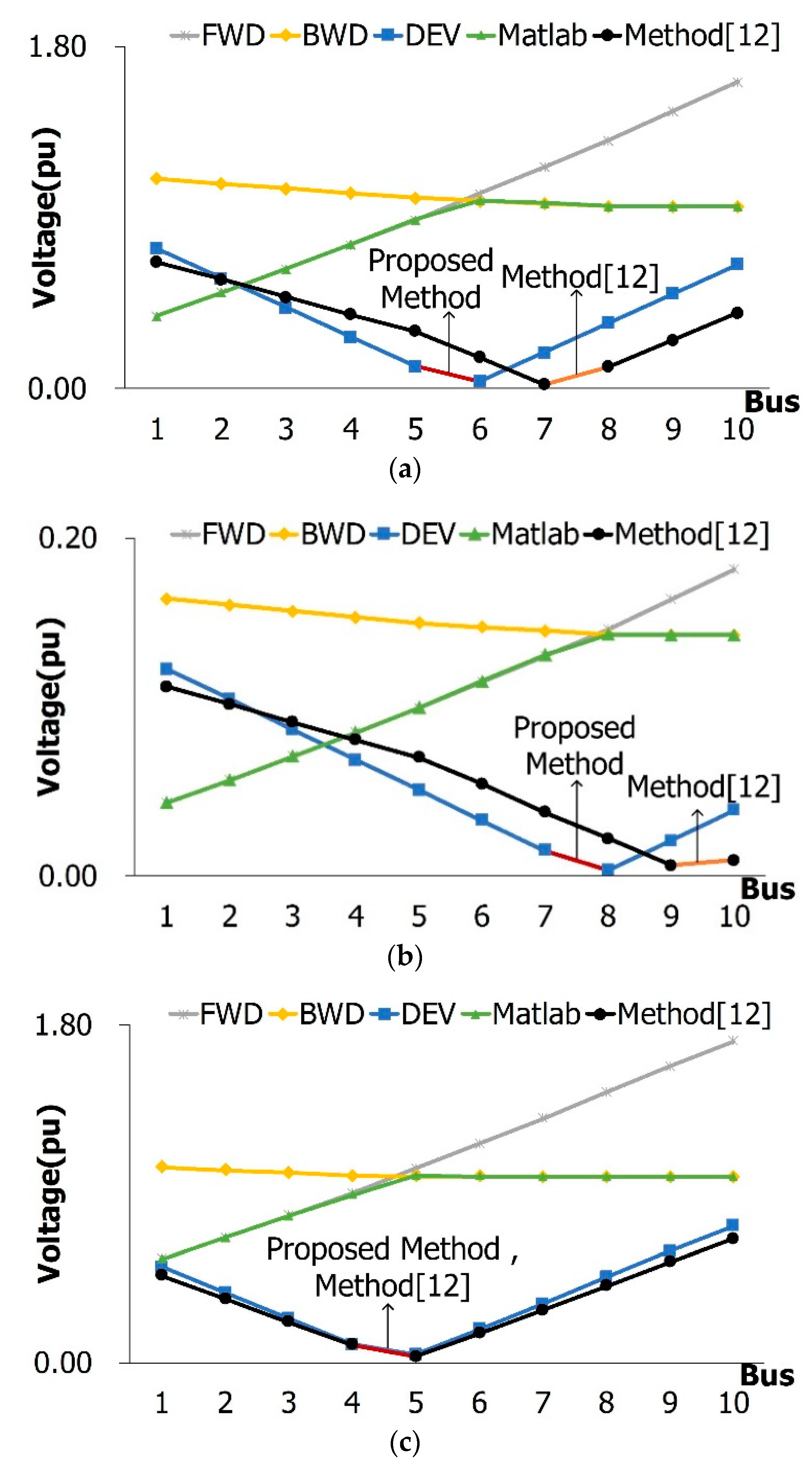
Figure 10 shows the results of the proposed algorithm under the fault of the main feeder. The actual fault location is marked in the red line, while the method [12] result is marked in the orange line. As shown in Figure 10, the proposed method calculated approximately the same results in the Matlab simulation. Consequently, the proposed method accurately identified the actual fault location. The existing study [12] did not consider the impact of the PVs and symmetrical components in the unbalanced faults, except the short circuit faults such as Figure 10c,d. Therefore, In Figure 10a,b, we could confirm that there was an error in estimating the fault location.

4.1.2. Stage 1 Estimation Results for the Error Test

To verify the robustness of the proposed method, we performed simulations for the error of network models and measurements. In the case of the network model, the proposed method could be affected by the error of the line parameters and the load estimation value. However, line parameter error (line length, phase information, etc.) was excluded from this paper because it was considered an improvement point of the utility’s operation and maintenance. To verify the effect of the load, the single line-to-ground fault with 30 Ω was simulated, and 1000 simulations were conducted for each fault location. Cases 1–3 include the error of 5%, 10%, and 15%, respectively. Table 5 shows the simulation results for the main feeder according to the load errors. It estimated a fault location to 100% in all cases. Various load estimation methods were proposed, as the Ref [1]. Therefore, it was considered that the occurrence of a slight error by load estimation methods would not be a big problem in the application of the proposed method.
Moreover, the robustness of the proposed method was verified for the measurement errors that could occur in the actual operation. The measurement error test was performed by applying noises to the voltage and current magnitudes of the RTU and PMU and the phasor angle measurements of the PMU. In Table 6, random errors were applied to the PMU and RTU measurement values (voltage and current magnitude) by protection class 3 specified by IEEE C57.13 and IEC 61869 [24,25]. The phasor angle errors of a voltage and current were also applied to the PMU by C37.118 [13]. For random error tests, we use a standard normal distribution. The range of standard deviation 3σ was applied to the error tests. The single line-to-ground fault was simulated, and 1000 simulations were conducted for each fault location. Cases 1–4 include the fault resistances of 0, 10, 20, and 30 Ω, respectively. The simulated fault locations were as follows: between Buses 2–3, 4–5, 6–7, and 7–8.
Although there were slight errors when the fault resistance was above 30 Ω, the accuracy of fault location was 100% for almost cases. Therefore, we confirmed that it is robust to the measurement error of Stage 1.
To verify the effect of the phasor angle error of a voltage and current measurement for PMUs during the main feeder fault, the case studies were performed based on Case 1 (0 Ω), which had the most volatile voltage and current variation among the above cases. Cases 1–4 added the phasor angle error of 0.57°, 1°, 2°, and 3° respectively. Table 7 shows the test results for the main feeder based on phasor angle errors. As a result, slight errors were recorded when the phasor angle error was above 3°, but the accuracy of fault location was almost 100% for all cases. Therefore, it was confirmed that the phasor angle error did not have a significant effect for fault location estimation of the main feeder.

4.2. Fault Location Estimation in the Lateral Feeder

4.2.1. Analysis of the Short Circuit Analysis Results

Table 8 presents the comparison results between the Matlab simulation results (“M”) and proposed short circuit analysis results (“C”). The single line-to-ground fault was simulated at every bus in the test system. The voltage and current values after the fault at the PMU points were comparatively analyzed. At the start and end of the feeder, the voltage and current were calculated at an error rate of approximately below 0.01%. Consequently, the proposed short circuit analysis method in this paper could calculate the variations of each bus before and after a fault, which were sufficiently applicable to the fault location in the lateral feeder.

4.2.2. Estimation Result of Stage 2

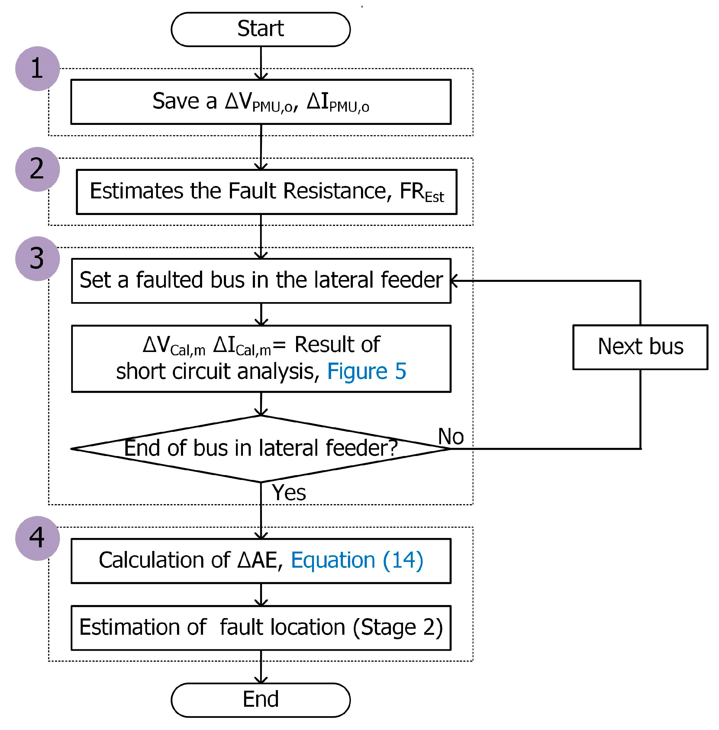
To verify the proposed algorithm of Stage 2, the faults were simulated for the lateral feeder. 
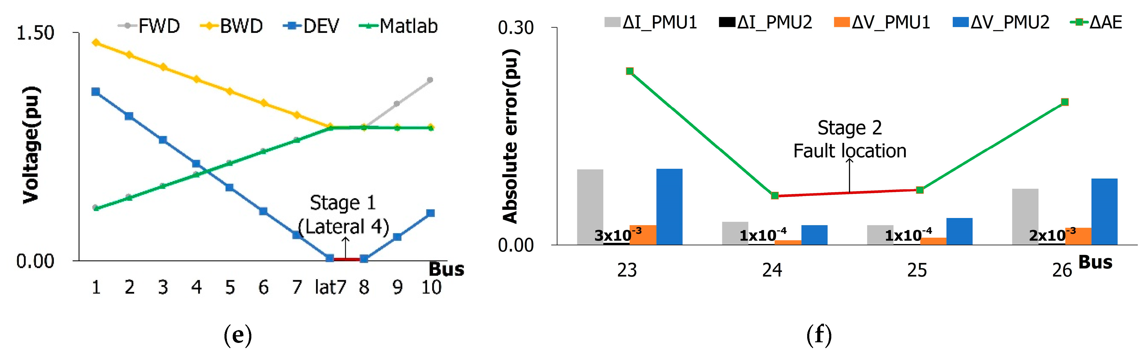
Figure 11 shows the results of fault location. Figure 11a,c,e shows the estimation results of Stage 1. In Figure 11b,d,f, Δ AE denotes the sum of absolute errors by using Equation (14). Δ I _ PMU and Δ V _ PMU , Δ δ _ PMU , Δ φ _ PMU are absolute errors between the calculated and measured values. ∆I_PMU2 is close to zero because it only affected by the load at the downstream of the PMU installation point. The fault simulation results demonstrated that Stage 1 estimated accurate fault locations for buses connected to the lateral feeder in every case. For calculation of the absolute errors in (14), if the estimated faulted resistance is less than 5 Ω, only the magnitude comparison is used. And in cases of more than 5 Ω, the entire Equation (14) is used. The criteria of fault resistance can be determined by short circuit analysis before applying the proposed algorithm to the target networks. In the case of Figure 11b,f, the magnitude comparison is only used because the estimated fault resistance is 0.065 Ω, 0.11 Ω, respectively. Through these results, it can be confirmed that the faulted section is accurately estimated because the magnitude deviation between buses is large when the fault resistance is small. In the case of Figure 11d, it can be seen that the magnitude and the phasor angle are compared because the estimated fault resistance is 29.875 Ω. The faulted section is accurately estimated according to the phasor angle deviation between buses. Therefore, it is necessary to consider not only the magnitude but also the phasor angle when a large fault resistance is inserted. As a result, Stage 2 confirms the accurate identification of the faulted sections in the lateral feeder.

4.2.3. Stage 2 Estimation Results for the Error Test

To verify the effect of Stage 2 for the load error, the same error test as the main feeder was conducted. Table 9 shows the results of the fault location for the lateral feeder according to the load errors. The proposed method estimates a fault location to 100% in all cases for the lateral feeder. As a result, the error of the load did not significantly affect the proposed method.
Moreover, to verify the robustness of the algorithm against random measurement errors caused by a fault in a lateral feeder. The measurement error test was also performed by applying noises to the voltage and current magnitudes of the RTU and PMU and the phasor angle measurements of the PMU for the main and lateral feeder. The single line-to-ground fault was simulated between buses 11–12, 17–18, 20–21, and 23–24. Table 10 presents the noise test results. In Stage 1, the accuracy of the fault location was near 100% because the fault within a lateral feeder shows the same phenomenon as that of the fault in the connection point of the lateral feeder. In the test results of Stage 2, the accuracy of fault location was approximately 100% when the fault point resistance was below 20 Ω. The minimum accuracy of fault location was 97.6% when a fault includes the fault point resistance of 30 Ω. Case 4 has an insignificant current and voltage of magnitude and phasor angle deviations between the buses under the fault condition. Accordingly, the measurement noise as more influential in Case 4 than in other cases. However, the main feeder buses connected with the lateral feeder that occurred in the error of estimation were identified to be close to 100% by Stage 1. It will not be an important problem because the distance of the lateral feeder is short when the restoration of actual distribution networks.
Table 11 shows the result of the fault location when additional PMU was installed in the lateral feeder 3. As a result, the fault location result was estimated to be close to 100% for the lateral feeder 3. Therefore, the number of PMUs was reduced compared to the existing method, and a similar effect could be obtained when additional PMUs were installed only in the lateral feeder having a low fault location estimation rate.
To verify the effect of the phasor angle error for the lateral feeder, the same phasor angle error test conducted. Table 12 shows the phasor angle error test results for the lateral feeder. As shown in Table 12, 2° or higher phasor angle errors began to influence the faulted section estimation result. However, this will not be a problem when applying the proposed algorithm because the maximum phasor angle error is 0.57° in Ref. [13,26], which is the specification of a commercial PMU product.

5. Conclusions

To improve the excessive installation of PMUs, which is a common problem of existing PMU-based fault location methods, this study proposed a 2-stage fault location estimation method that combined the PMU measurements and short circuit analysis. In Stage 1 of the fault location in the main feeder, the symmetrical components of the voltage and current variations were considered to deal with the unbalanced fault. It also considered the impact of the lateral feeder with large-capacity DER on the main feeder. In Stage 2 of the fault location in a lateral feeder, the faults at each point in the lateral feeder were analyzed by using a short circuit analysis based on the unbalanced power flow that considers the dynamic control characteristics of the PV inverter. Then, the short circuit analysis results were compared with the measurement values at the installation point of PMU. As mentioned above, the proposed method requires the simultaneous measurement of PMU installed points (both ends of the main feeder and additional points as needed). This is common to Stage 1 for fault location estimation in the main feeder and Stage 2 for comparing the short circuit analysis value and the measurement. Accordingly, we used the PMU because simultaneous measurements require the voltage, current, and phasor angle. We could use the PQ meter or other instruments if they satisfy this requirement.
The following conclusions on the proposed algorithm were derived.
(1) The results of stage 1—where the fault location was simulated under diverse fault situations in the main feeder—were very similar to the Matlab simulation results. As compared with the existing study [12], the fault location was more accurate. Accordingly, the proposed method proved to be more effective as it considered unbalanced faults and the impact of DERs in the lateral feeder.
(2) In the results of Stage 2, it was confirmed that two buses with the smallest deviation between the short circuit analysis results considering the dynamic characteristics of the PV inverter and measured value of PMU were identified as the fault locations. Accordingly, unlike the existing PMU-based fault location methods, the proposed algorithm did not require the installation of additional PMUs and prevented an excessive number of PMUs from being installed in the distribution networks.
(3) To verify the robustness of the proposed method, we performed the simulations for the error of network models and measurements. In the case of the network model, we believed that the elements of the parameter errors that influence the proposed method are line parameters and load estimation data. The errors of the line parameters such as line length and phase are expected to influence every system analysis method and operation algorithm. However, this should be researched as a separate topic because the line parameter errors are considered an improvement point of the utility’s operation and maintenance. In recently, the grid modernization and the introduction of new operating system (advanced DMS) due to the increased complexity of the distribution network are promoting the correction of line parameter errors. When using the RTU as in this study, load values can be estimated more accurately by the RTU measurement and state estimation as shown in reference [1]. Moreover, as shown in the results of case study by load estimation error in Table 5 and Table 9 in this study, the proposed method shows robust results even in load values with a 15% error. Therefore, we believed that the load estimation error will not be a problem in applicability of the proposed method.
The test of measurement errors was performed by applying noises to the voltage and current magnitudes of the RTU and PMU and the phasor angle measurements of the PMU. The magnitude and phasor angle errors were applied based on the standard and product specifications of References [13] and [24,25,26]. For random error tests, the standard normal distribution that has the range of standard deviation 3σ was applied. In the measurement noise test, every fault case for the main feeder showed an accuracy of approximately 100%. In the fault cases of the lateral feeder, the accuracies were about 100% when the fault point resistance was 20 Ω and below. The fault location was identified with a minimum accuracy of 97.6% when the fault point resistance was 30 Ω. This can be seen to occur because the deviation for the magnitude of voltage and current and phasor angle between the buses was very small due to the fault resistance. However, the main feeder connected buses with the lateral feeder performed an estimation close to 100%. This will not be a big problem because the distance of the lateral feeder is short when there is restoration of the actual distribution networks. The fault location result is also estimated to be close to 100% for the lateral feeder 3 when additional PMU is installed at the end of lateral feeder 3. Therefore, the number of PMUs is reduced compared to the existing method, and similar effects can be obtained when additional PMUs are installed only in the lateral feeder having a low fault location estimation rate. As shown in the test results for phasor measurement error, 2° or higher phasor angle errors influenced the fault location estimation result. However, this will not be a problem when applying the proposed algorithm because the maximum measurement error of phasor angle is 0.57° in Ref. [13,26], which is the specification of a commercial PMU product.
(4) The most remarkable advantage of the proposed method can be summarized as follows. The existing studies require the installation of many PMUs to estimate the impact of PVs and a fault location in the lateral feeder. The proposed method can achieve the same effect by using two PMUs at the main feeder, the RTUs, and the short circuit analysis method. The installation of additional PMUs causes a communication cost and infrastructure burden for the operation of distribution systems. As pointed out above, the proposed method will reduce the communication cost and accomplish accurate fault locations. These are significant improvements. Two problems that are worthy of notice still exist. First, the distribution networks are regularly reconfigured once or twice a year to ensure a load balance in each season and secure fault restoration reserves. For this reason, the locations of the PMUs installed at both ends of the main feeder may change. However, if the change of the PMU installation point from the reconfiguration of the distribution network may be excluded, the proposed method is sufficiently applicable to the actual distribution network.
Second, the proposed method estimates the fault location by adding minimum PMUs in an existing network where RTUs are installed. Therefore, the proposed method can be applied to the systems where automation of the distribution system is applied (urban systems in Asia (including South Korea, Japan, Hong Kong, Singapore, etc.), Europe, and North America). However, we assumed the installation of RTUs for large capacity DER (such as PV), and applied the output ratio of large-capacity PV for small-capacity PVs. Hence, the cost can be increased by the installation of additional RTUs. However, this additional cost can be sufficiently covered by the actual operation because: (1) The PV output has a significant effect on the voltage and other problems recently in the operation of the distribution network. Therefore, the measurement of PV output is increasingly important for real-time operation of the distribution network (monitoring and control) and for establishing operation planning through PV output prediction. (2) The range of fault location can be reduced from the section with remote controlled switch to the section with manual switch. Furthermore, the fault location can be identified through data transfer between PMUs, which has the advantage of shortening the isolation time of the faulted section and the restoration time of the un-faulted sections. As mentioned above, the grid modernization and the introduction of new operating system also justify the additional installation of these new measuring devices.
Additionally, according to IEEE 1547 [27], DER is tripped after a voltage abnormally is detected for anti-islanding. This standard specifies the minimum trip time as 0.16 s (10 cycles). However, the PV trip will not have a significant effect because the faulted section estimation using the PMU measurements uses measurements of much faster time than the time mentioned above.
The management of distribution networks becomes a more complicated task due to the DERs. The improvement in reliability is one of the essential purposes for managing a distribution network. If the results of this study are utilized for network restoration in association with the distribution network management or for the agent-based fault recovery through device-to-device communication the reliability of distribution network will be more significantly improved than before.

Author Contributions

J.-S.H. prepared the manuscript and implemented the theory and simulations. S.-Y.Y. supervised the study and discussed the results. G.-D.S., J.-H.C. and S.-J.A. analyzed the simulation results and commented on the manuscript. All authors have read and agreed to the published version of the manuscript.

Funding

This research was funded by Korea Electric Power Corporation. (Grant number: R18XA04). This research was funded by the Korea Institute of Energy Technology Evaluation and Planning (KETEP) and the Ministry of Trade, Industry and Energy(MOTIE) of the Republic of Korea (No. 2019381010001B).

Conflicts of Interest

The authors declare no conflict of interest.

References

  1. Yun, S.-Y.; Chu, C.-M.; Kwon, S.-C.; Song, I.-K.; Choi, J.-H. The development and empirical evaluation of the Korean smart distribution management system. Energies 2014, 7, 1332–1362. [Google Scholar] [CrossRef] [Green Version]
  2. Seo, J.-S.; Kim, H.-S.; Lim, S.-I.; Choi, M.-S.; Lee, S.-J. An improved algorithm of fault indicator generation of FRTU in distribution automation system. Trans. Korean Inst. Electr. Eng. 2014, 63, 1354–1363. [Google Scholar] [CrossRef] [Green Version]
  3. Lee, H.-S.; Jeon, C.-W.; Kim, Y.-K.; Lim, S.-I. Faulted section identification method in the distribution systems with renewable energy resources. Trans. Korean Inst. Electr. Eng. 2014, 63, 1321–1327. [Google Scholar] [CrossRef] [Green Version]
  4. Eaton. Available online: https://www.eaton.com/ecm/groups/public/@pub/@nederland/@elec/documents/content/pct_495064.pdf (accessed on 18 February 2020).
  5. Teng, J.H.; Huang, W.H.; Kuan, S.W. Automatic and fast faulted line-section location method for distribution systems based on fault indicators. IEEE Trans. Power Syst. 2014, 29, 1653–1662. [Google Scholar] [CrossRef]
  6. Sun, K.; Chen, Q.; Gao, Z. An automatic faulted line section location method for electric power distribution systems based on multisource information. IEEE Trans. Power Deliv. 2016, 31, 1542–1551. [Google Scholar] [CrossRef]
  7. Dzafic, I.; Jabr, R.A.; Henselmeyer, S.; Ðonlagić, T. Fault location in distribution networks through graph marking. IEEE Trans. Smart Grid 2018, 9, 1345–1353. [Google Scholar] [CrossRef]
  8. Liao, Y. Generalized fault-location methods for overhead electric distribution systems. IEEE Trans. Power Deliv. 2011, 26, 53–64. [Google Scholar] [CrossRef]
  9. Bahmanyar, A.; Jamali, S. Fault location in active distribution networks using non-synchronized measurements. Int. J. Electr. Power Energy Syst. 2017, 93, 451–458. [Google Scholar] [CrossRef]
  10. Dashti, R.; Daisy, M.; Shaker, H.R.; Tahavori, M. Impedance-based fault location method for four-wire power distribution networks. IEEE Access 2017, 6, 1342–1349. [Google Scholar] [CrossRef]
  11. Usman, M.U.; Faruque, O. Validation of a PMU-based fault location identification method for smart distribution network with photovoltaics using real-time data. IET Gener. Transm. Dis. 2018, 12, 5824–5833. [Google Scholar] [CrossRef]
  12. Farajollahi, M.; Shahsavari, A.; Stewart, E.M.; Mohsenian-Rad, H. Locating the source of events in power distribution systems using micro-PMU data. IEEE Trans. Power Syst. 2018, 33, 6343–6354. [Google Scholar] [CrossRef] [Green Version]
  13. IEEE. Standard for Synchrophasor Data Transfer for Power Systems; IEEE: Piscataway, NJ, USA, 2011. [Google Scholar]
  14. Available online: www.powerstandards.com/wp-content/uploads/dlm_uploads/2017/10/Introduction-to-microPMU.pdf (accessed on 18 February 2020).
  15. Park, J.-Y.; Jeon, C.-W.; Lim, S.-I. Accurate section loading estimation method based on voltage measurement error compensation in distribution systems. J. Korean Inst. Illum. Electr. Install. Eng. 2016, 30, 43–48. [Google Scholar]
  16. Biswal, M.; Brahma, S.M.; Cao, H. Supervisory protection and automated event diagnosis using PMU data. IEEE Trans. Power Deliv. 2016, 31, 1855–1863. [Google Scholar] [CrossRef]
  17. Liang, X.; Wallace, S.A.; Nguyen, D. Rule-based data-driven analytics for wide-area fault detection using synchrophasor data. IEEE Trans. Ind. Appl. 2017, 53, 1789–1798. [Google Scholar] [CrossRef]
  18. Castilla, M.; Miret, J.; Sosa, J.L.; Matas, J.; de Vicuna, L.G. Grid fault control scheme for three-phase photovoltaic inverters with adjustable power quality characteristics. IEEE Trans. Ind. Electron. 2010, 25, 2930–2940. [Google Scholar] [CrossRef]
  19. Plet, C.A.; Green, T.C. Fault response of inverter interfaced distributed generators in grid connected applications. Electr. Power Syst. Res. 2014, 106, 21–28. [Google Scholar] [CrossRef]
  20. Chen, T.H.; Chen, M.S.; Hwang, K.J.; Kotas, P.; Chebli, E.A. Distribution system power flow analysis a rigid approach. IEEE Trans. Power Deliv. 1991, 6, 1146–1152. [Google Scholar] [CrossRef]
  21. Kersting, W.H. Distribution System Modeling and Analysis, 2nd ed.; CRC Press: Boca Raton, FL, USA, 2007; pp. 83–89. [Google Scholar]
  22. Xiao, P.; Yu, D.C.; Yan, W. A unified three-phase transformer model for distribution load flow calculations. IEEE Trans. Power Syst. 2006, 21, 153–159. [Google Scholar] [CrossRef]
  23. Choi, J.-H.; Park, D.-H. Mid-to-Long Term Operation Plan of Distribution Control Center According to Expansion of Distribution System Intelligent Equipment; Final Report; KEPCO: Naju, Korea, 2017; pp. 14–38. [Google Scholar]
  24. IEEE. Standard Requirements for Instrument Transformers; IEEE: Piscataway, NJ, USA, 2016. [Google Scholar]
  25. IEC. Instrument Transformers—Part 2: Additional Requirements for Current Transformers; IEC: Geneva, Switzerland, 2012. [Google Scholar]
  26. Micro-PMU Data Sheet. Available online: https://www.powerstandards.com/download-center/micropmu/ (accessed on 18 February 2020).
  27. IEEE. Standard for Interconnection and Interoperability of Distributed Energy Resources with Associated Electric Power Systems Interfaces; IEEE: Piscataway, NJ, USA, 2018. [Google Scholar]
Figure 1. Outline of the phasor measurement unit (PMU)-based fault location method [11].
Energies 13 01294 g001
Figure 2. Outline of the PMU-based fault location method [12].
Energies 13 01294 g002
Figure 3. Overall flow chart of the proposed fault location method.
Energies 13 01294 g003
Figure 4. Flowchart of the proposed fault location method (Stage 1).
Energies 13 01294 g004
Figure 5. Flowchart of the dynamic fault analysis.
Energies 13 01294 g005
Figure 6. Three-phase admittance configuration of a distribution network under a fault.
Energies 13 01294 g006
Figure 7. Flowchart of the proposed fault location method (Stage 2).
Energies 13 01294 g007
Figure 8. Test system for the case studies. (a) Test model of the Korea active distribution test system (KADTS). (b) Modified test system.
Energies 13 01294 g008
Figure 9. Modeling of a PV system. (a) PV system in Simulink. (b) PV control characteristics in the fault condition.
Energies 13 01294 g009
Figure 10. Fault location results under a fault in the main feeder, (a) single line-to-ground between Buses 5 and 6, (b) single line-to-ground between Buses 7 and 8 (resistance of fault point is 30 Ω), (c) Line-to-line between Buses 4 and 5, and (d) three-phase fault between Buses 4 and 5.
Energies 13 01294 g010aEnergies 13 01294 g010b
Figure 11. Results of fault location for the single line-to-ground fault between Buses 12 and 13, (a) Stage 1 and (b) Stage 2, result of fault location for single line-to-ground fault between Buses 16 and 17 (30 Ω), (c) Stage 1 and (d) Stage 2, result of fault location for three-phase fault between Buses 24 and 25, (e) Stage 1 and (f) Stage 2.
Energies 13 01294 g011aEnergies 13 01294 g011b
Table 1. Monthly amount of accumulated data for each terminal unit.
Type of MeterRTUPMUSmart Meter
Amount of data/cycles1/2 s10–120 s1/15 min
Acquisition data typeP, Q, V (m), I (m), θ V I , etc.P, Q, V (m, δ ),
I (m, θ ), etc
P, V, etc.
Accumulated data generation/month44.2 MB1.13–13.45 GB0.41 MB
Required
communication speed
132 bps3.36–40.32 kbps1.227 bps
Table 2. Communication cost for PMU data transfer ($/month).
Data Transfer Samples (s)1060120
Type of communicationNB-IOT83.91562.171136.94
LTE13.8413.8420.77
Table 3. Set values for photovoltaics (PVs).
TypePV1PV2PV3PV4PV5PV6
Capacity0.5 MVA0.1 MVA2 MVA0.1 MVA0.2 MVA1 MVA
Maximum current/Rated current1.21.21.21.21.21.2
TransformerYg/YgYg/△Yg/△Yg/YgYg/YgYg/△
Capacity typeLargeSmallLargeSmallSmallLarge
Table 4. Comparison of fault location results under a single line-to-ground fault.
Variation of Bus Δ V 1 Δ V 2 Δ V 3 Δ V 4 Δ V 5 Δ V 6 Δ V 7 Δ V 8 Δ V 9 Δ V 10
Proposed MethodFWD0.2970.3890.4830.5780.6870.7960.9051.0151.1401.264
BWD1.1341.1061.0791.0521.0361.0221.0070.9930.9930.993
DEV0.8490.7240.6010.4770.3520.2280.1040.0250.1470.272
Proposed Method (W/O PV)FWD0.2970.3890.4830.5780.6740.7710.8670.9641.0611.158
BWD0.9980.9970.9960.9950.9940.9940.9930.9930.9930.993
DEV0.7140.6160.5180.4200.3230.2250.1280.0310.0680.165
Method in [12]FWD0.2970.3590.4220.4860.5510.6160.6820.7480.8140.881
BWD0.9970.9960.9950.9940.9940.9930.9930.9930.9930.993
DEV0.7120.6460.5790.5120.4460.3790.3120.2450.1790.112
Matlab Simulation0.2970.3900.4840.5790.6880.7980.9080.9930.9930.993
Lateral Δ I l a t e r a l 2 f a u l t e d   p h a s e Δ I l a t e r a l 4 f a u l t e d   p h a s e
Type Δ I Δ φ Δ I Δ φ
Proposed Method0.0669147.16150.0758137.5514
Matlab Simulation0.0667148.01010.0758137.4807
Notes: The shaded parts in Table 4 show the estimated fault section for each method.
Table 5. Accuracy of the fault location according to load errors (fault in the main feeder).
CasesCase1Case 2Case 3
5%10% 15%
Fault Location Stage1Stage1Stage1
2–3100%100%100%
4–5100%100%100%
6–7100%100%100%
7–8100%100%100%
Table 6. Accuracy of the fault location according to measurement noises (fault in the main feeder).
TypeCase1Case 2Case 3Case 4
0 10   20   30  
Fault Location Stage 1Stage 1Stage 1Stage 1
2–3100%100%100%100%
4–5100%100%100%99.2%
6–7100%100%100%100%
7–8100%100%100%99.1%
Table 7. Accuracy of the fault location according to phasor angle error (fault in the main feeder).
TypeCase1Case 2Case 3Case 4
0.57°
Fault Location Stage 1Stage 1Stage 1Stage 1
2–3100%100%100%100%
4–5100%100%100%99.8%
6–7100%100%100%100%
7–8100%100%100%99.9%
Table 8. Comparison between the fault analysis and Matlab simulation.
Bus48112124
Type Mag. (A)Ang. (Deg)Mag. (A)Ang. (Deg)Mag. (A)Ang. (Deg)Mag. (A)Ang. (Deg)Mag. (A)Ang. (Deg)
M V PMU 1 6777.218.849531.323.685719.517.469695.223.9210146.024.74
C V PMU 1 6766.018.639522.823.565712.017.239687.123.8110139.624.65
Error (%)0.0020.0110.0010.0050.0010.0130.0010.0050.0010.004
M V PMU 2 634.326.605.6098.783947.921.294893.224.652342.825.43
C V PMU 2 627.126.755.49100.013928.720.954882.824.522339.825.32
Error (%)0.0110.0060.0200.0120.0050.0160.0020.0050.0010.004
M I PMU 1 4258.3−47.532471.3−43.204916.3−49.582365.4−42.862065.4−42.25
C I PMU 1 4272.5−48.552483.8−44.134928.9−50.632377.1−43.772075.9−43.17
Error (%)0.0030.0210.0050.0220.0030.0210.0050.0210.0050.022
M I PMU 2 0.3026.600.002798.761.8821.292.3324.651.1225.43
C I PMU 2 0.3026.750.0026100.011.8720.952.3324.521.1225.32
Error (%)0.0000.0060.0370.0130.0050.0160.0000.0050.0000.004
Table 9. Accuracy of the fault location according to load errors (faults in lateral feeder).
ErrorCase 1Case 2Case 3
5%10%15%
Fault Location Stage 1Stage 2Stage 1Stage 2Stage 1Stage 2
11–12100%100%100%100%100%100%
17–18100%100%100%100%100%100%
20–21100%100%100%100%100%100%
23–24100%100%100%100%100%100%
Table 10. Accuracy of fault location according to the measurement noises (faults in lateral feeder).
CaseCase 1Case 2Case 3Case 4
Fault Location
0 Ω10 Ω20 Ω30 Ω
Stage 1Stage 2Stage 1Stage2Stage 1Stage 2Stage 1Stage 2
11–12100%100%100%100%100%100%100%98.8%
17–18100%100%100%100%100%100%100%99.7%
20–21100%100%100%100%100%100%100%97.6%
23–24100%100%100%100%100%100%100%98.4%
Table 11. Accuracy of fault location according to the installation of PMU in the lateral feeder 3.
CaseCase 1Case 2Case 3Case 4
0   10   20   30  
Fault Location Stage 1Stage 2Stage 1Stage 2Stage 1Stage 2Stage 1Stage 2
20–21100%100%100%100%100%100%100%100%
Table 12. Accuracy of fault location according to the phasor angle error (faults in lateral feeder).
CaseCase 1Case 2Case 3Case 4
0.57°
Fault Location Stage 1Stage 2Stage 1Stage 2Stage 1Stage 2Stage 1Stage 2
11–12100%100%100%100%100%100%100%100%
17–18100%100%100%100%100%100%100%100%
20–21100%100%100%100%100%100%98.9%97.9%
23–24100%100%100%100%100%100%99.1%95.7%

