Phase Synchronization Stability of Non-Homogeneous Low-Voltage Distribution Networks with Large-Scale Distributed Generations

Abstract

The ideal distributed network composed of distributed generations (DGs) has unweighted and undirected interactions which omit the impact of the power grid structure and actual demand. Apparently, the coupling relationship between DGs, which is determined by line impedance, node voltage, and droop coefficient, is generally non-homogeneous. Motivated by this, this paper investigates the phase synchronization of an islanded network with large-scale DGs in a non-homogeneous condition. Furthermore, we explicitly deduce the critical coupling strength formula for different weighting cases via the synchronization condition. On this basis, three cases of Gaussian distribution, power-law distribution, and frequency-weighted distribution are analyzed. A synthetical analysis is also presented, which helps to identify the order parameter. Finally, this paper employs the numerical simulation methods to test the effectiveness of the critical coupling strength formula and the superiority over the power-law distribution.

1. Introduction

Renewable energy sources have a broad prospect in power systems these days—more and more distributed generations (DGs) are integrated into the modern electricity grid. The distributed generation has the advantages of being environmentally-friendly and sustainable. In addition, two weaknesses include low output power per unit and energy output in remote areas that can not be ignored. For one thing, the low output power per unit of solar power and wind power results in a low capacity for one DG unit. This is why the distribution network requires a large number of installed DGs to provide effective output power. For another thing, the remote distribution leads to power systems usually working in the islanded operation. Different from the normal generators, there is no rotor in the DGs such as batteries and photovoltaic units. That is to say, the frequency stability is easy to be broken in the islanded microgrid composed of DG units without the rotating mass [1,2,3]. Hence, we will address the issue of phase and frequency stability in the islanded system.

Previous studies have based their criteria for selection on the local control of a few DGs in the ideal model [4,5,6]. Reference [7] shows the change of various parameters of generators in a large scale photovoltaic system and presents two different operations to research the voltage stability in an IEEE 30-bus model with a Large-Scale photovoltaic module. Indeed, the large-scale photovoltaic module can be considered as one high-capacity DG in the case of IEEE 30-bus, and no method of improving stability was given in [7]. Conventionally, when the number of composed DG increases, the active low-voltage islanded network will face the issue of high-order, multi-dimensional, and strong coupling. In brief, with a sharp increase in the number of DGs, the system will encounter the problem named “Curse of Dimensionality”. Therefore, it is difficult for previous solutions that consider a few DGs to address relevant problems in current research effectively.

We note that recently there has been some advanced complex network theory that provides the stability analysis of large-scale network systems. It has wide applications in cyber science [8], medical science [9], social science [10], and so on. Nevertheless, there are a few related studies on the frequency stability of an active distribution network composed of DG units.

In addition, previous research mainly assumes that the networks are unweighted and undirected; this means that the coupling relationship between nodes has no direction, and the strength of all couplings is consistent. However, this assumption mismatches the characteristics of the real network of many cases. For instance, in an active distribution network, the coupling relationship between DGs which takes droop control is determined by the node voltage, line impedance, and droop coefficient, where the line impedance between DGs is generally determined by the distance between DGs. Apparently, the assumption that all DGs in the active distribution network is equidistant is undoubtedly harsh and impractical. On the contrary, the assumption that the coupling relationship between DGs is non-homogeneous is more realistic. Fortunately, complex network theory has made a difference in weighted networks. Reference [11] investigates the system of Kuramoto oscillators whose weight is related with a degree in the asymmetrical situation and comes to one conclusion that the critical coupling strength has a positive correlation with the degree exponent. Reference [12] indicates that the degree sequence contributes to the ability to synchronize in the mean field. Reference [13] shows that the degree distribution of the fixed system has a negative degree correlation between its nodes, which improves its synchronizability. Besides the weighted methods with the degree, some other papers pay attention to the weighted methods with frequency. Reference [14] introduces a weighting method which cares about the relationship between frequency and link to achieve the phase synchronization. Linear and nonlinear weighting procedures are applied in mean and heterogeneous systems to verify the method. Frequencies of symmetrical oscillators are studied in the bipolar model built by [15], while the relationship between frequency and coupling strength is analyzed. Reference [16] comes to the conclusion that asymmetric weights that depend on loads make contributions to the stability of the whole system. Overall, weighted methods that are based on the inherent qualities of the inverter nodes [17,18], i.e., node degrees [19], node loads [20], and network’s global properties in the connection links have been discussed widely to enhance the network synchronization in recent studies.

However, the general impact of weighted coupling on network synchronization is not studied comprehensively, especially the weighted method. These weighted procedures above, unfortunately, are designed only concerned with the inherent attributes of the network, i.e., the size of the nodes degree or the edges between vertices, which limits their applications. Thus, these weighted procedures may have a significant difference from real systems. Therefore, it is important to describe such real weighted distribution methods in weighted networks.

Thereby, it is of great importance to study different weighted distribution methods of a distribution network, which has not been discussed yet. This paper employs some weighted distribution methods that are found in many realistic networks such as the link weight and investigates the phase synchronization performance in a large-scale islanded network to pave the way for the solution of the similar weighted distribution issues in the future. The innovations of this paper are as follows.

(1)

We derive non-homogeneous models for simulating different weighted distribution methods in a large-scale islanded distribution network.

(2)

We analytically study the effects of weighted distribution methods on the phase synchronization stability by means of explicit synchronization conditions. We illustrate our insightful results and the utility of our approach through the critical coupling strength formula.

(3)

Different from other studies focusing on the weighted distribution methods which only associate with the inherent properties of the network, this paper adopts several realistic distribution styles as weighted distribution methods to research the synchronization stability in the large-scale distribution network.

The rest of this paper is organized as follows. In Section 2, we introduce correlation complex network theory. Section 3 focuses on the modeling of weighted distribution and derivation of the critical coupling strength formula. The numerical results and simulation analyses in Section 4 are used to compare the network stability of different weighting methods. Section 5 concludes this paper.

2. Correlation Theory

The structure of an active distribution network can be achieved by mirroring algebraic graph theory. Furthermore, the synchronization condition of an active distribution network will be analyzed by order parameters that are introduced thoroughly in the following. Then, the critical coupling strength of network stability can be obtained with the help of synchronization condition.

2.1. Graph Theory

The microgrid can be modeled as a graph G, where $V=\{{\theta }_1,{\theta }_2,\cdots {\theta }_N\}$ is the set of edges while $E\in V\times V$ is the set of edges. Generally, the connected graph can be called an undirected graph when $({\theta }_i,{\theta }_j)$ and $({\theta }_j,{\theta }_i)$ represent the same edge. The value of weight $a_{ij}$ defines whether the graph is weighted ($a_{ij}\ne 1$) or not ($a_{ij}=1$) and hence we have the associated adjacency matrix $A=\left[a_{ij}\right]$. Moreover, the Laplace matrix L is a symmetric zero-sum matrix of undirected graphs, where $l_{ii}={\sum }_{i\ne j}{a}_{ij}$, $l_{ij}=-a_{ij}$. The matrix L satisfies:

$$\left\{\begin{array}{c}{l}_{ij}\le 0,i\ne j\hfill \\ \sum _{j=1}^N{l}_{ij}=0,i=1,\cdots ,N\hfill \end{array}\right.$$

(1)

Whether the graph G is a directed graph or an undirected graph, its associated matrix is based on a directed label, which means edge $e=\{i,j\}\in E$ is represented by an ordered pair $(i,j)$. In the undirected graph, we assign an arbitrary direction to it. For the ordered pair $(i,j)$, we define $b_{je}=1$ if j is the sink node of edge e, $b_{ie}=-1$ if i is the source node of edge e, and $b_{ke}=0$ otherwise in the incidence matrix $B=\left[b_{ie}\right]\in R^{n\times m}$. In addition, the edge $(i,j)$ satisfy ${\left(B^{T}X\right)}_e=x_j-x_i$.

2.2. Synchronization Conditions

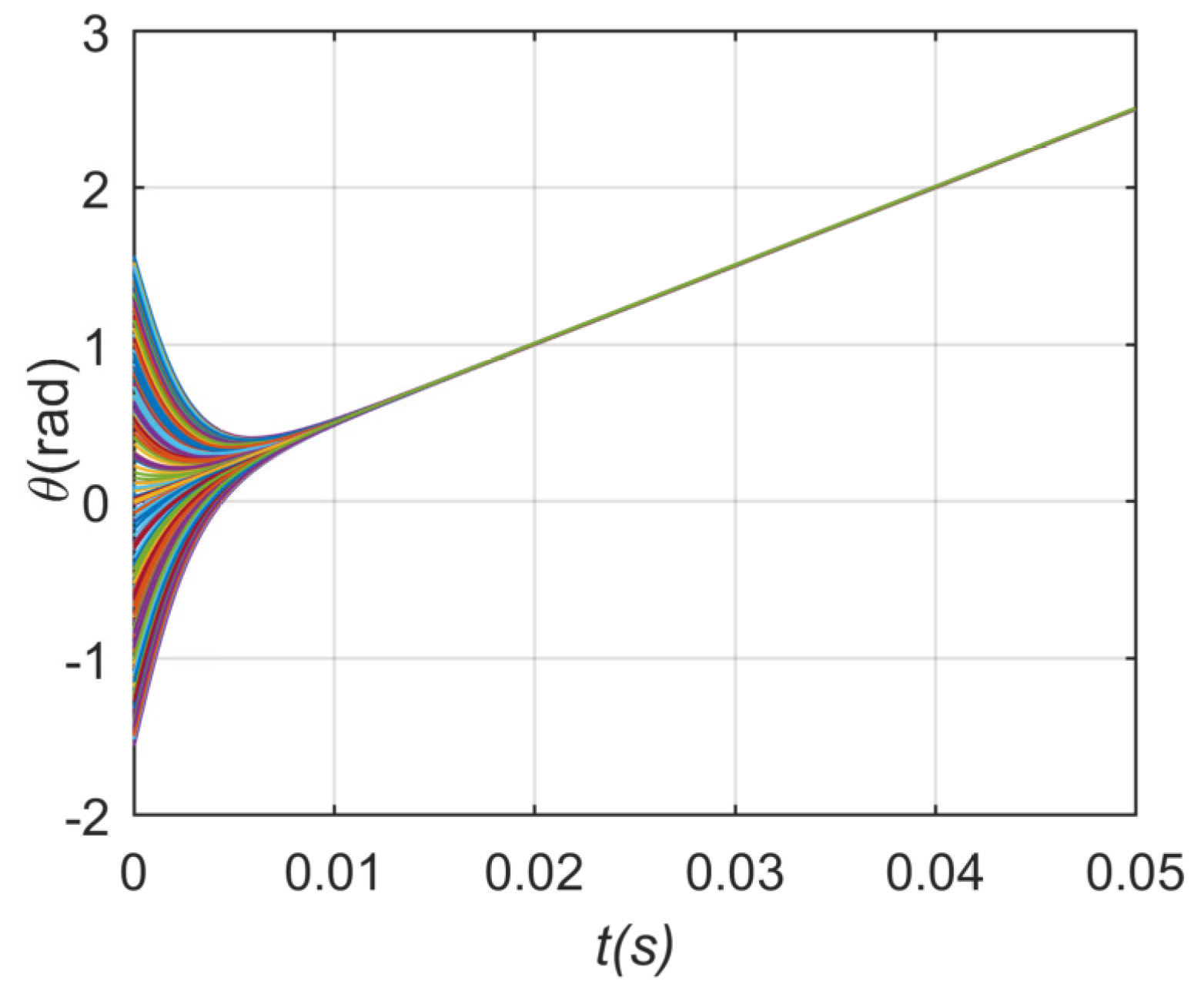
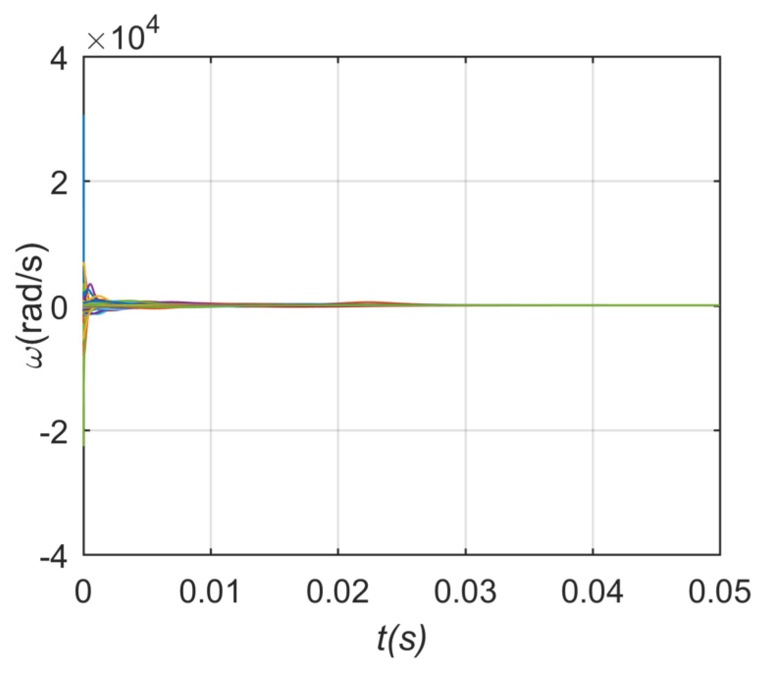
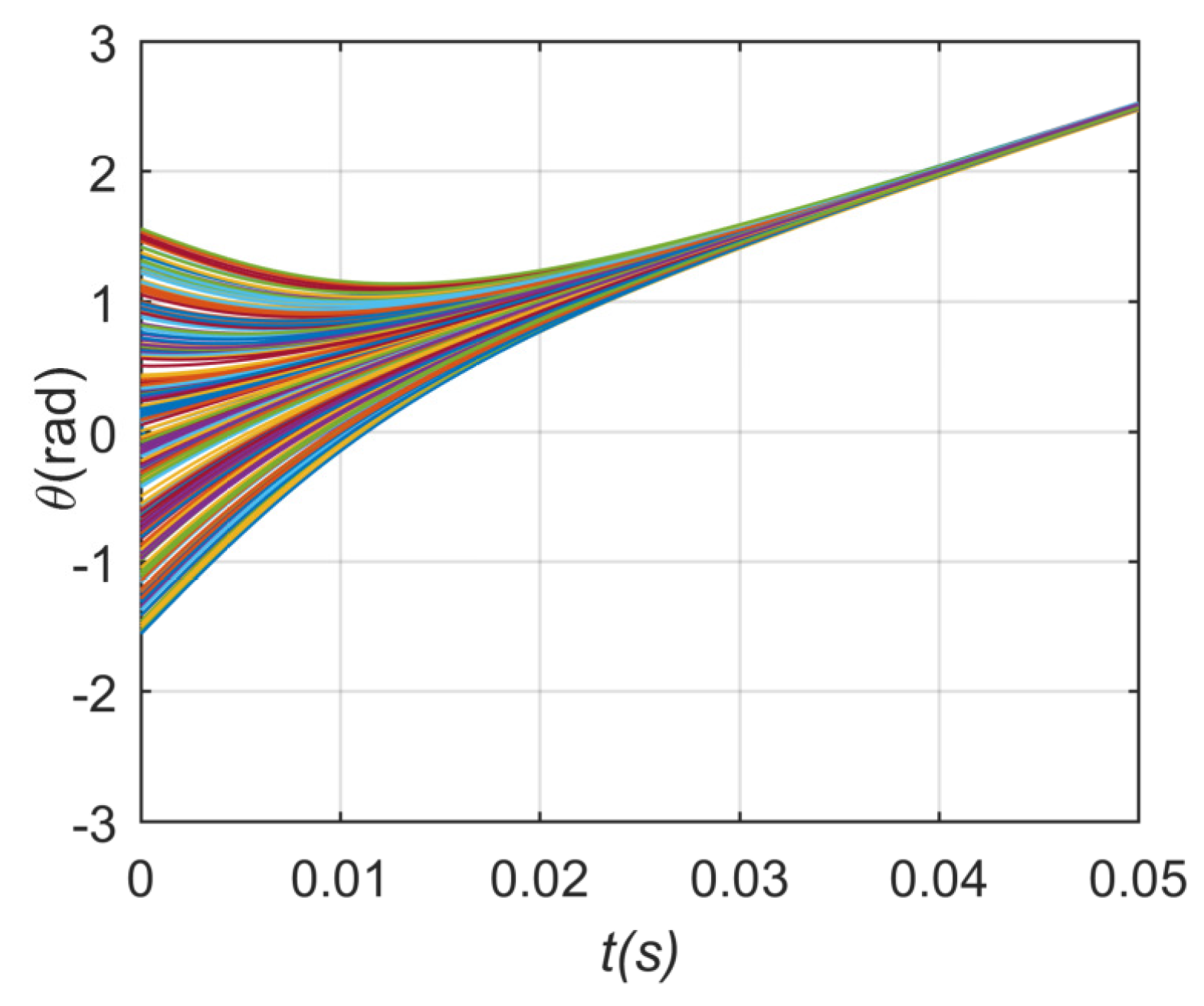
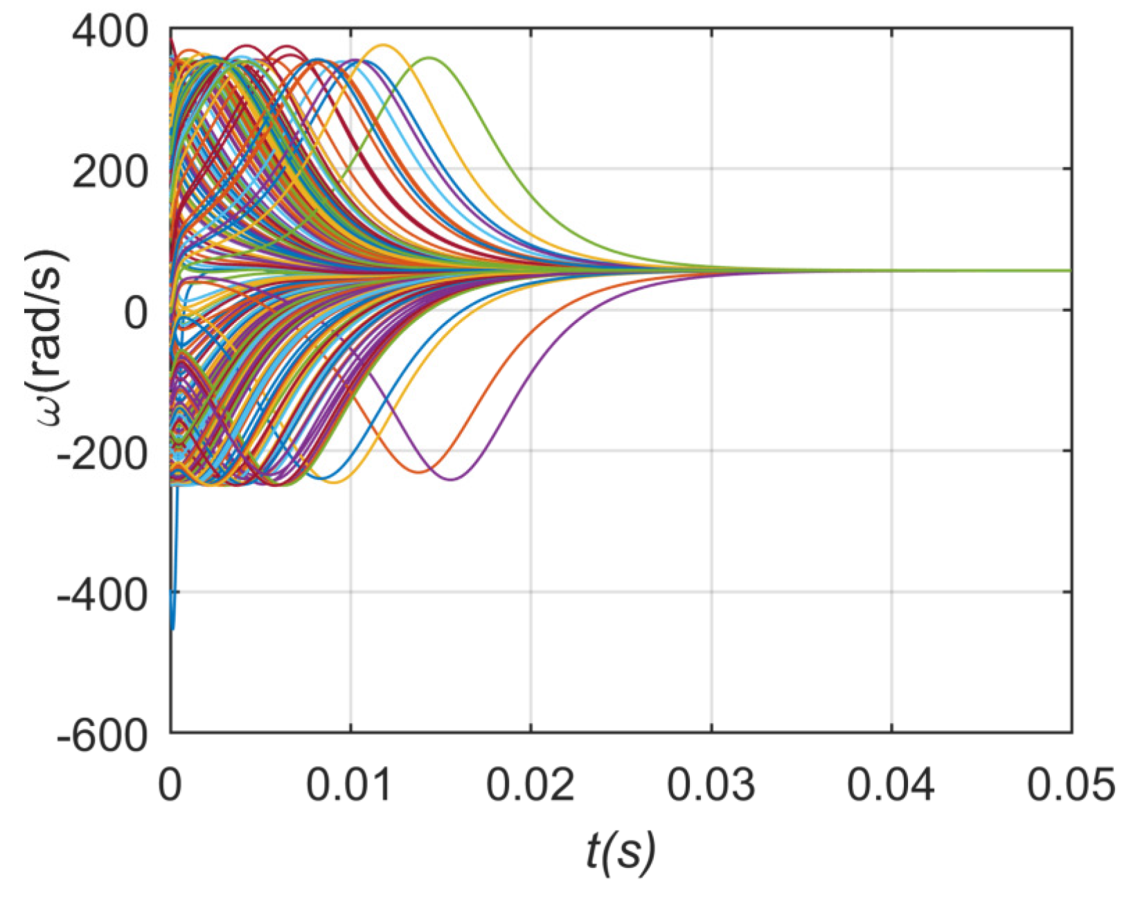
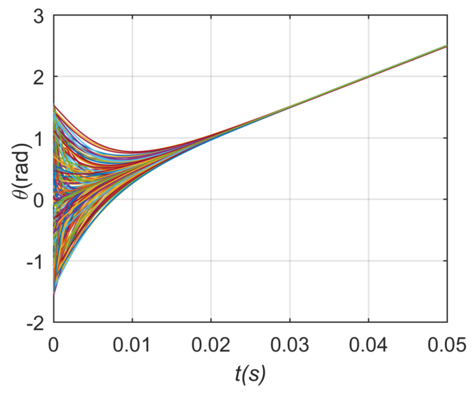
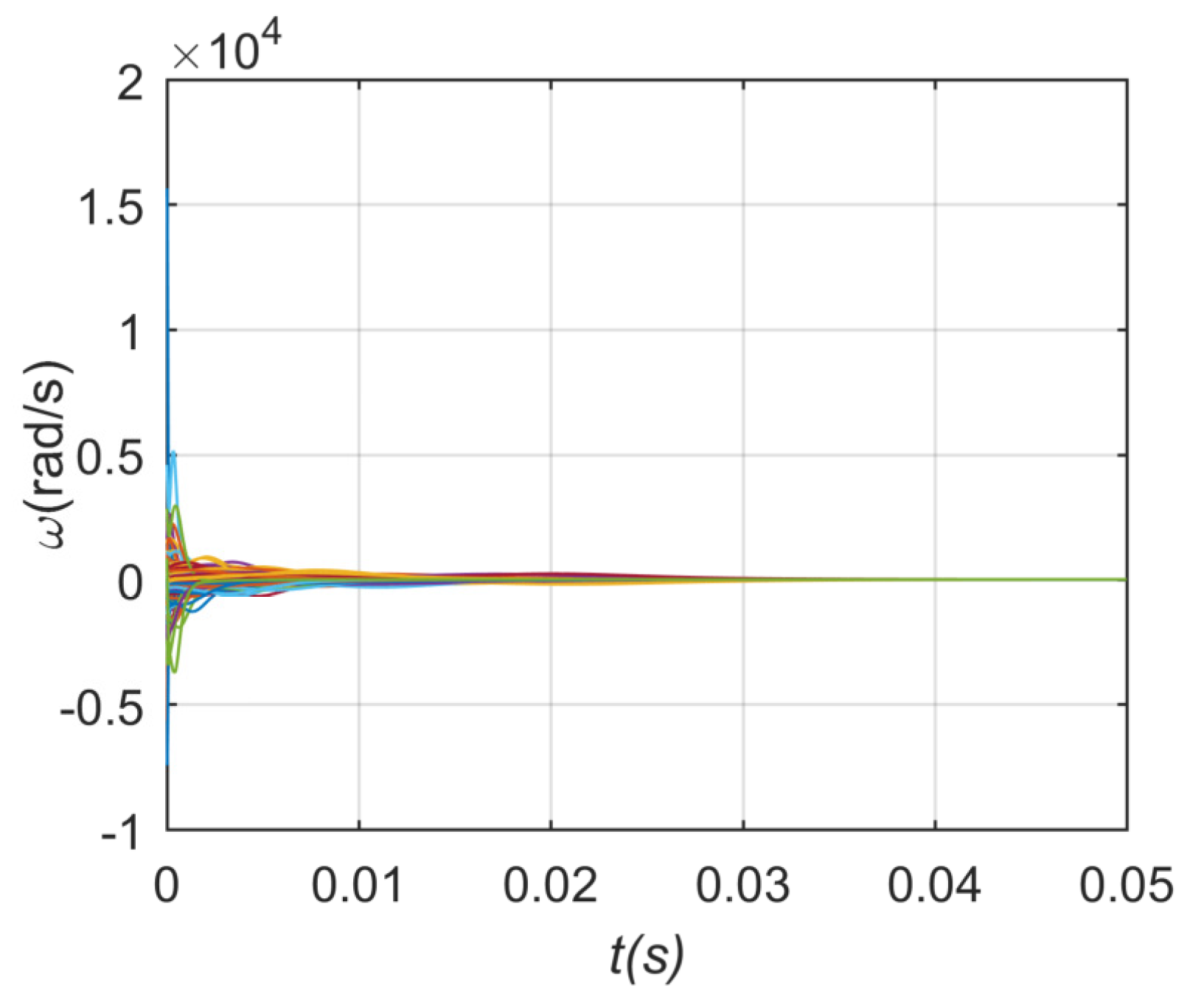
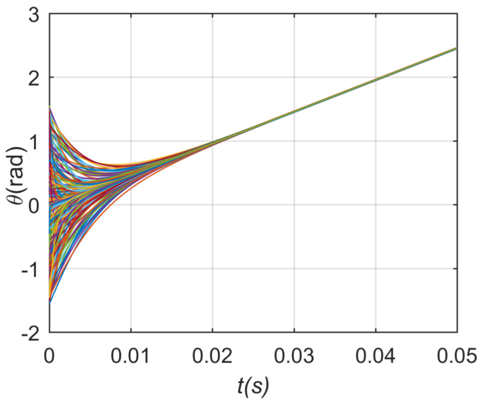
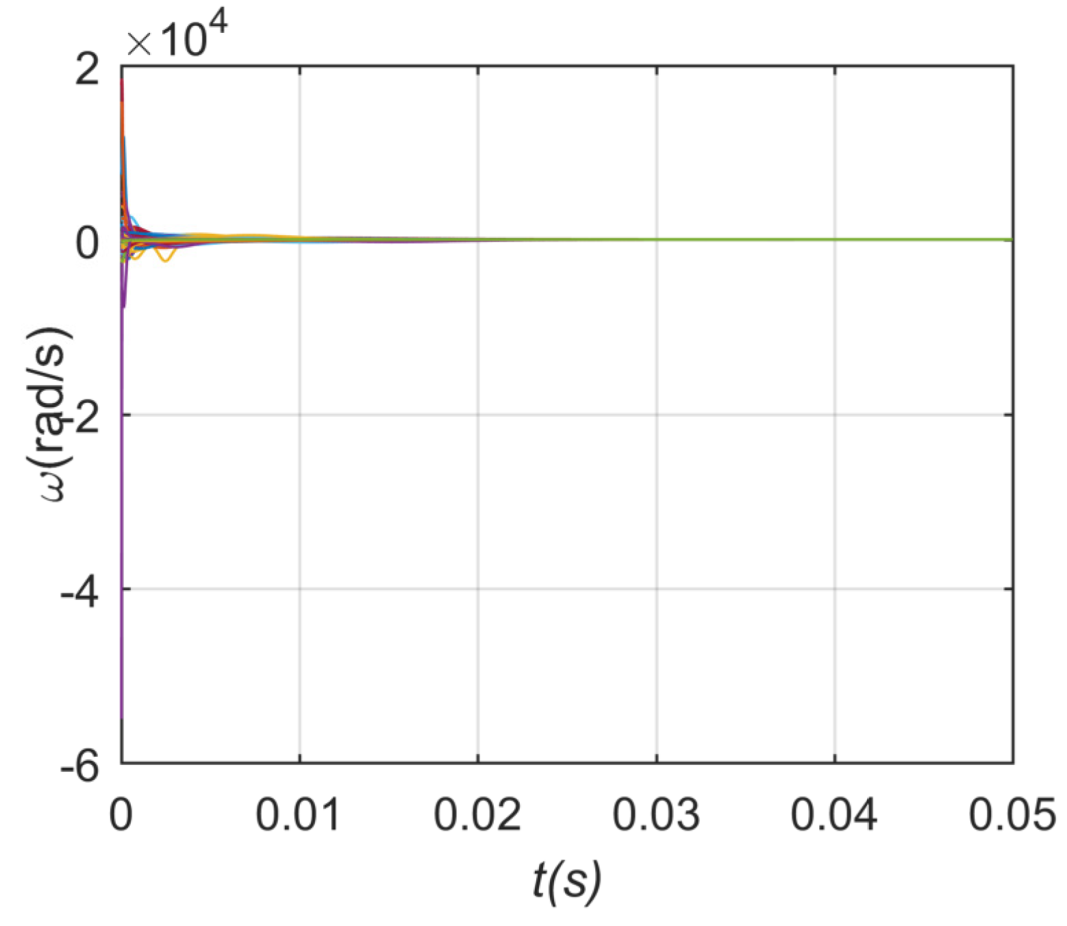
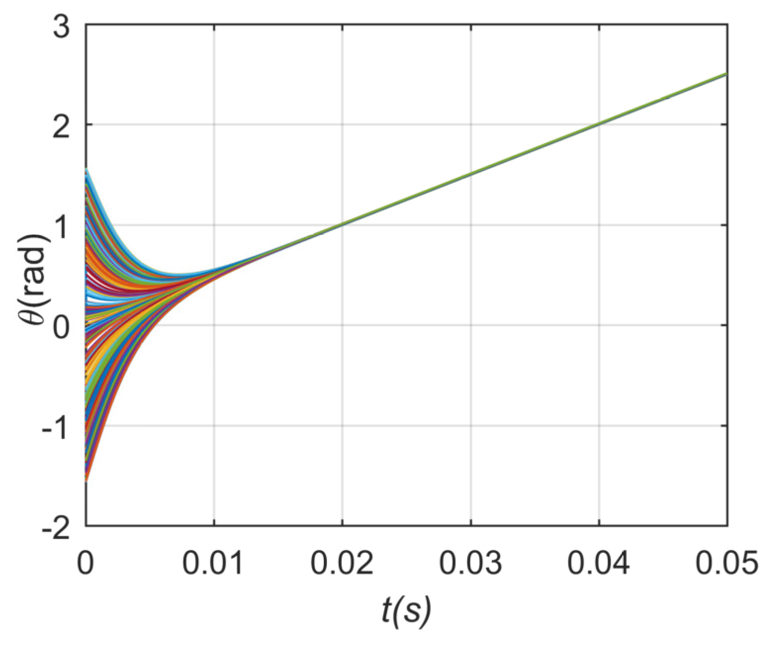
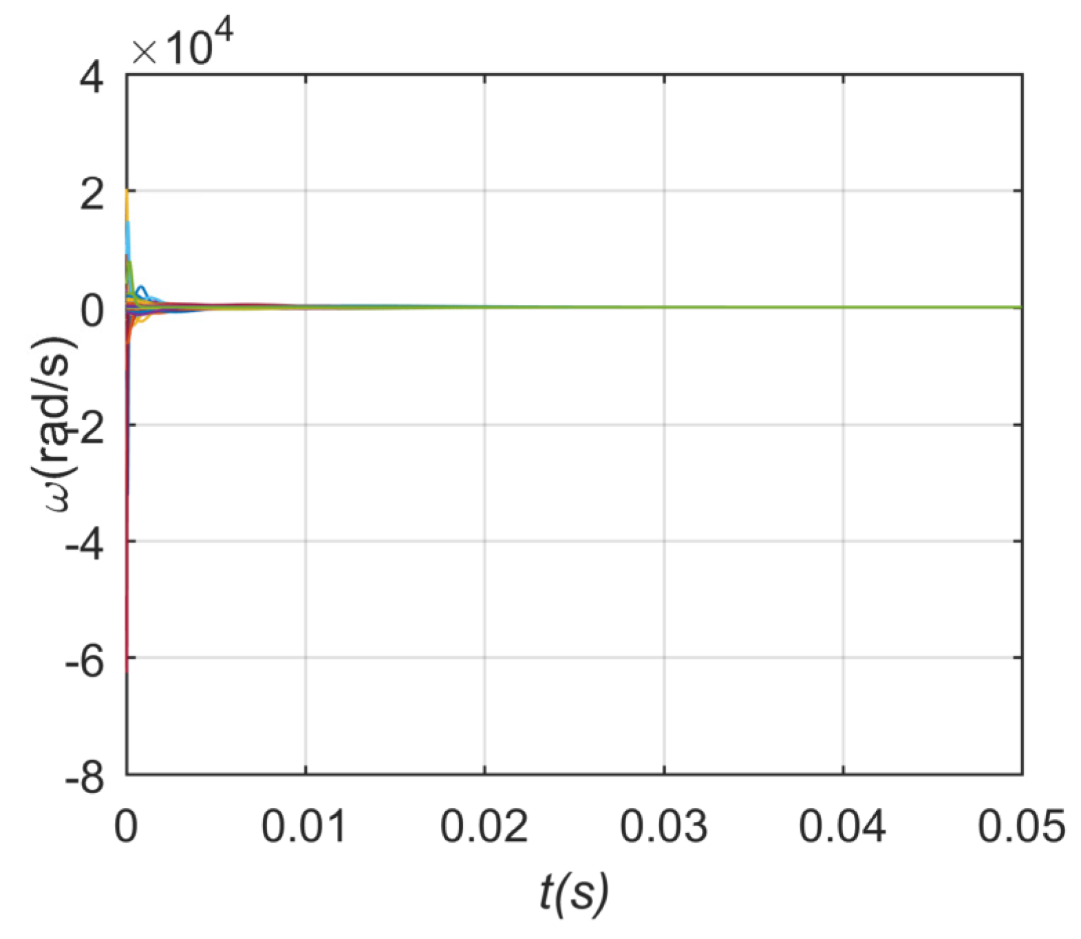
Specifically, the phase and frequency of all DG units tend to stabilize at a fixed value when $t\to \infty$. Therefore, we focus on the synchronization process of phase and frequency to research the system stability intuitively.

If the coupling strength K between the DG nodes in a complex network is larger than the critical value $K_{cr}$, the DG nodes will divide into two groups, the phase of one cluster is fixed at a stable specific frequency while the other oscillators have a drift.

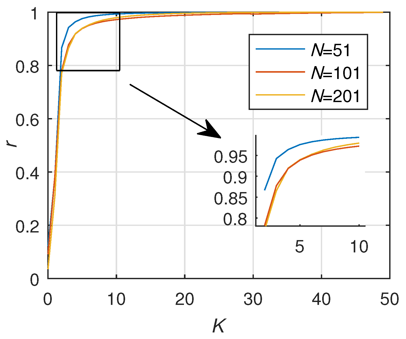
The order parameter is a visual signal to show the change of phase, whose definition is:

$$r{e}^{i\psi }=\frac{1}{N}\sum _{j=1}^N{e}^{i{\theta }_j}$$

(2)

The size of r shows the percentage of stable nodes. The value is:

$$\left|r\right|=\frac{1}{N}\left|\sum _{j=1}^N{e}^{i{\theta }_j}\right|$$

(3)

where $r=1$ means that a system enters a stable state absolutely while $r=0$ means that a system becomes unstable.

Criterion 1 [21]: For a complex network graph G with an incidence matrix B, each pair of interconnected oscillators $\{i,j\}\in \epsilon$ could enter frequency synchronization and phase convergence $\left|{\theta }_i-{\theta }_j\right|\le \gamma <\pi /2$ when satisfying

$${∥L^{†}\omega ∥}_{\epsilon ,\infty }:={∥B^T{L}^{†}\omega ∥}_{\infty }\le sin\left(\gamma \right)$$

(4)

where $L^{†}$ is the inverse of Laplace matrix L, $\omega =({\omega }_1,\cdots {\omega }_n{)}^T$ is the vector of the natural frequency of each oscillator in the network and ${∥·∥}_{\epsilon ,\infty }$ evaluates the worst-case dissimilarity of this weighted projection.

This paper will use this synchronization condition to obtain the critical coupling strength of network synchronization under weighted conditions.

2.3. Critical Coupling Strength

In the previous subsection, the synchronization conditions recently mentioned in [22] have been introduced. In different occasions, these conditions have been proven to be applicable to oscillator models. This paper takes the Kuramoto oscillator to express the nonlinear ordinary differential equations:

$${\dot{\theta }}_i={\omega }_i+\sum _{j\in N_i}{a}_{ij}sin({\theta }_j-{\theta }_i),i=1,2,3...N$$

(5)

The model can be expressed as a matrix:

$${\dot{\theta }}_i=\omega -BWsin\left(B^T{\theta }_i\right),i=1,2,3...N$$

(6)

$W:=diag\left(w\right)$ is the diagonal matrix of weights. In a complex network, which determines the stability of the system is not the absolute value of the phase but the phase difference. The network entry synchronizes only when two phases of coupled nodes ${\phi }_1$ and ${\phi }_2$ are locked at a certain ratio, which means $\left|n{\phi }_1-m{\phi }_2\right|<$constant. Therefore, the phase difference vector is $\phi \left(t\right):=B^T\theta$, and the Equation (6) can be expressed by the phase difference:

$$\dot{\phi }=B^T\omega -B^{T}BWsin\left(\phi \right)$$

(7)

In the above equation, the synchronous solution can be expressed as $\dot{\phi }=0$ or $\dot{\phi }={\phi }^{\ast }$ for a fixed point ${\phi }^{\ast }\in R^n$.

In an analysis of [23], Fazlyab found that all fixed points of Equation (7) can be expressed as:

$$sin\left({\phi }^{\ast }\right)=W^{r-1}{B}^T{\left(B{W}^r{B}^T\right)}^{†}\omega +W^{-1}Fy$$

(8)

where $F\in R^{m\times m-n+1}$ is a matrix whose columns span the null space of B, i.e., $BF=0$, $y\in R^{m-n+1}$, and r is an arbitrary real number.

When $F=0$ and the fixed point ${\phi }^{\ast }$ is unique, the particular solution $W^{r-1}{B}^T{\left(B{W}^r{B}^T\right)}^{†}\omega$ is independent of r. In the special case of $r=0$, we have that

$$sin\left({\phi }^{\ast }\right)=B^T{L}^{†}\omega$$

(9)

provided that ${∥B^T{L}^{†}\omega ∥}_{\infty }\le 1$.

This section has proposed the theory about synchronization. The next section will analyze the situation of different weighting methods in star topology through algebraic graph theory, and obtain the critical coupling strength by using the synchronization condition.

3. Weighted Distribution

The weighted distribution is not only helpful to describe the features of real networks but are also crucial for controlling network synchronization. Three different weighting methods will be discussed to research the phase synchronization of a large-scale islanded network in this section. This issue takes an ideal star topology as the research object. Furthermore, a critical coupling strength formula for the weighted star network would be proposed first in this paper.

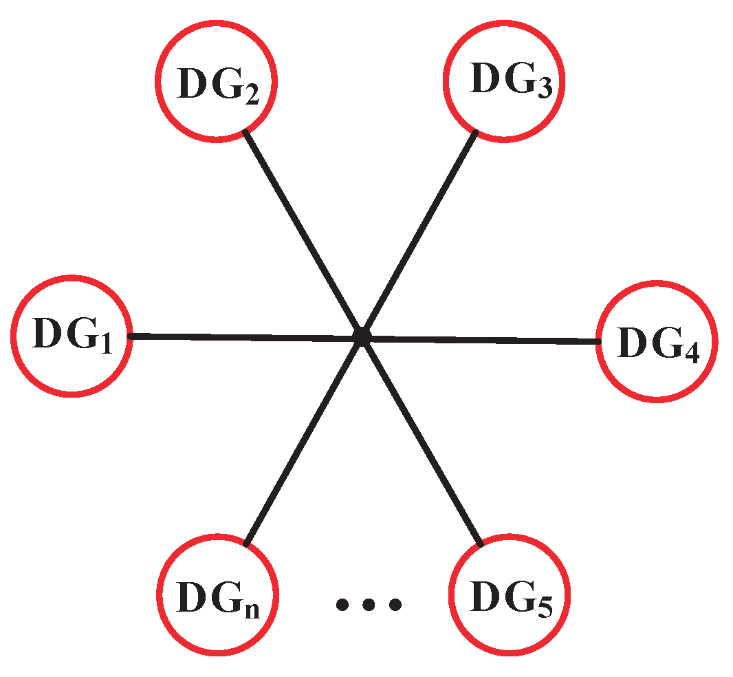
3.1. Star Topology

The purpose of this investigation is to explore the synchronization stability of large-scale grid-tied DG in islanded operation. Considering that most of the distribution networks are star topology [24,25], this paper chooses star topology as the object, as shown in Figure 1. The star network is shaped by one primary node and many branch nodes connected with it. It is characterized by high reliability, easy operation, and easy maintenance when the branch lines fail. However, this structure will consume a lot of metal and switchgear. Therefore, it is suitable for important construction sites with large capacity equipment or special places with concentrated load and wet, corrosive environments [21,26,27].

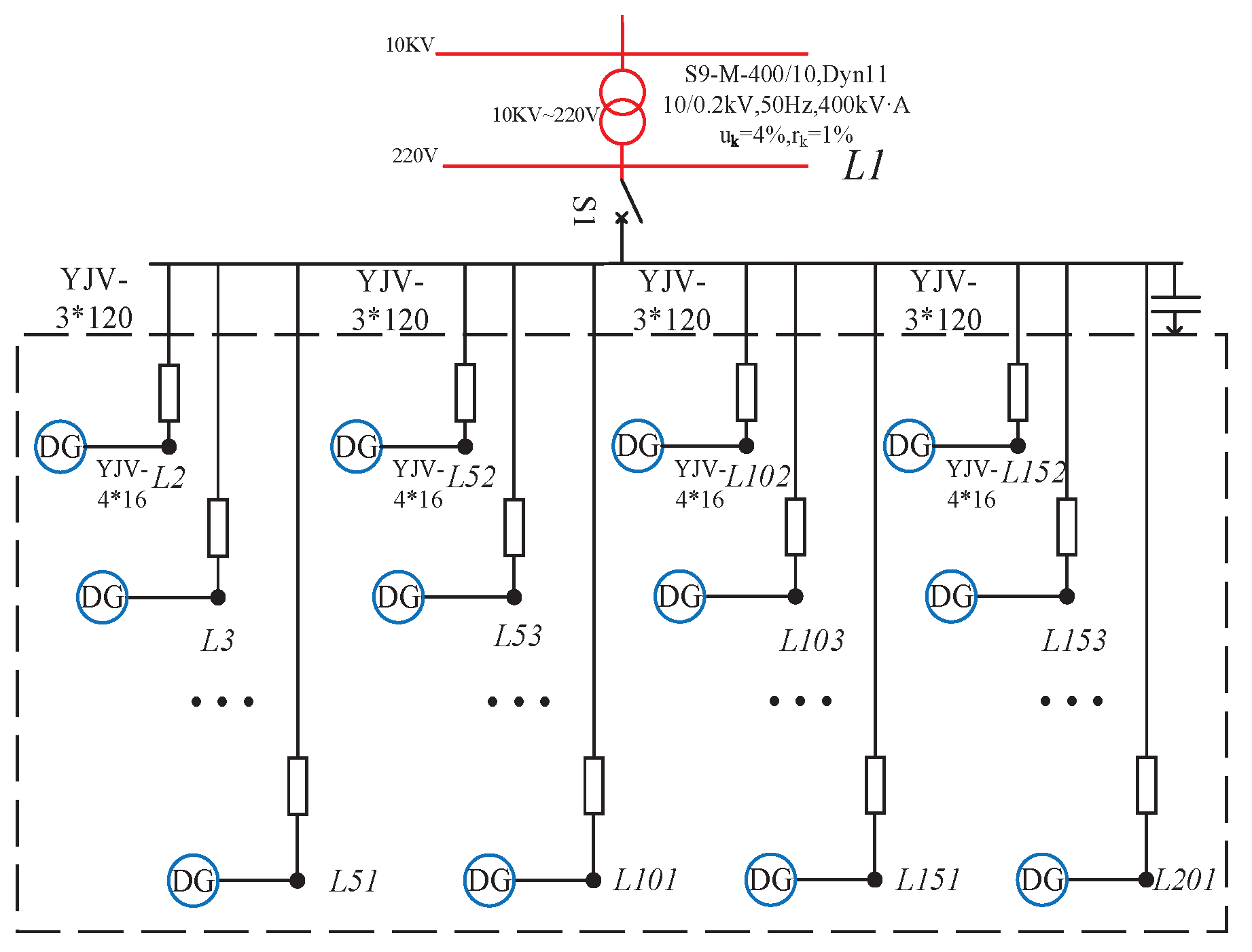
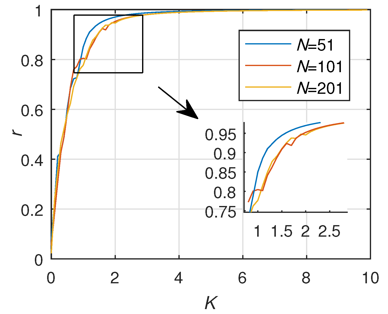
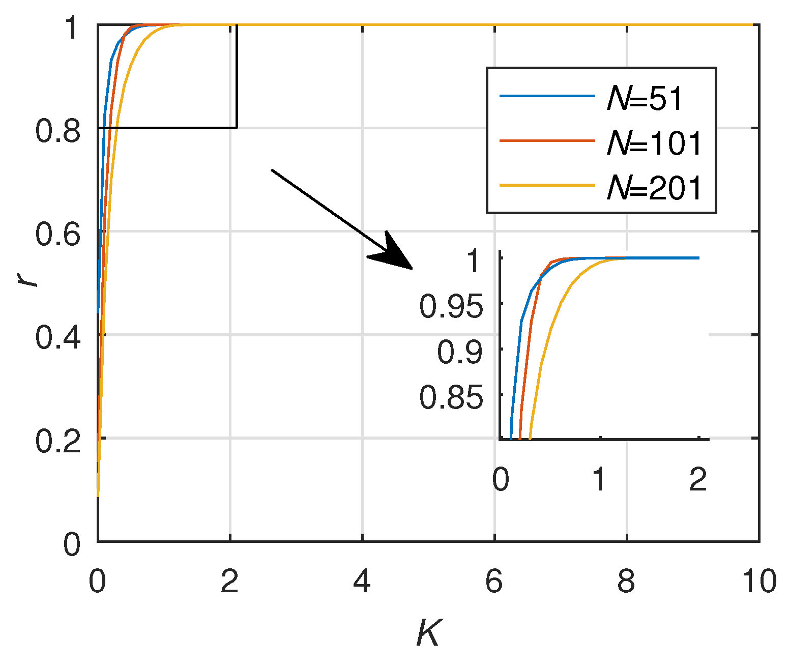
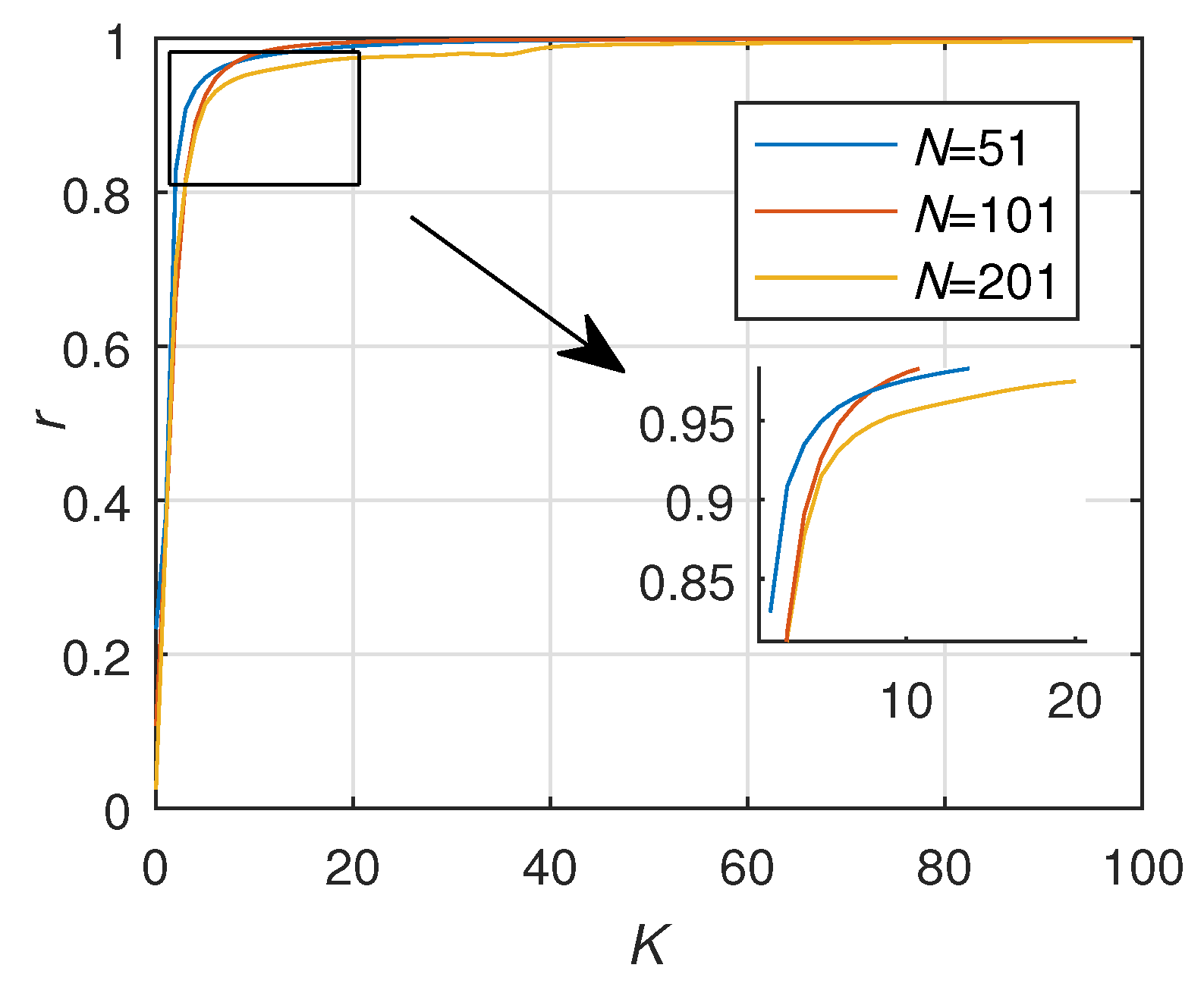
Due to the practical application of the power grid, the traditional research object of multi-machine (three to five machines) can no longer meet the actual needs. This is why this paper delivers an explicit analysis of the network stability with large-scale grid-tied DG. The number of DG N in a Large-scale model generally refers to $N\ge 200$, where this paper takes N as 201. There are no conventional generators with rotors used in this model, and all DGs are photovoltaic units. The photovoltaic community electrical diagram with star topology is depicted in Figure 2. We assume that the value of the line impedance between load nodes and the master node is consistent, and the inverter of each load node has the same impedance, so the impedance value between load node and the master node is equal. Therefore, $Z=Z_{line}+Z_{inv}$ and the admittance value is $Y=\frac{1}{Z}=\frac{1}{Z_{line}+Z_{inv}}$.

In Figure 2, each load node is only connected to the master node $L1$, and the impedance value between nodes $Z_{ij}=Z+Z_{inv}$ are equal. Therefore, the admittance matrix with star topology is

$$\begin{array}{c}\left|Y_{ij}\right|={\left[\begin{array}{cccc}0& \left|Y_{12}\right|& \cdots & \left|Y_{1N}\right|\\ \left|Y_{21}\right|& 0& \cdots & ⋮\\ ⋮& ⋮& ⋮& ⋮\\ \left|Y_{N1}\right|& \cdots & \cdots & 0\end{array}\right]}_{(N\times N)}\hfill \\ ={\left[\begin{array}{cccc}0& \left|\frac{1}{Z+Z_{inv}}\right|& \cdots & \left|\frac{1}{Z+Z_{inv}}\right|\\ \left|\frac{1}{Z+Z_{inv}}\right|& 0& \cdots & \dots \\ ⋮& ⋮& ⋮& ⋮\\ \left|\frac{1}{Z+Z_{inv}}\right|& \cdots & \cdots & 0\end{array}\right]}_{(N\times N)}\hfill \end{array}$$

(10)

3.2. The General Formula for Weighted Distribution

The DG units with droop control can be described as a Kuramoto oscillator [28,29,30]:

$$\begin{array}{c}\frac{d{\theta }_i}{dt}={\dot{\theta }}_t={\omega }_i-{\omega }_{\theta }=-m_i\left(p_i-p_{i\theta }\right)=m_i{p}_{i\theta }-m_i{p}_i\hfill \\ =m_i{p}_{i\theta }-m_i{E}_i{\sum }_{j=1}^n\left|Y_{ij}\right|E_{j}sin\left({\theta }_i-{\theta }_j\right)\hfill \end{array}$$

(11)

where $m_i{p}_{i\theta }={\omega }_i$, ${\omega }_i$ is the rated frequency of inverter in the ith DG node. In addition, the value of ${\omega }_i$ is chosen from the probability density function $g\left(\omega \right)$. When the standard frequency is 50 Hz, we take $g\left(\omega \right)$ as the symmetric normal distribution of 50, therefore $g\left(\omega \right)\sim (50,1)$.

In the above equation, the weight between $D{G}_i$ and $D{G}_j$ nodes is obtained by the droop coefficient $d_i$, the voltage of node $E_i$, $E_j$, and the admittance $\left|Y_{ij}\right|$. At this point, the coupling strength

$$K_i=d_i\left|Y_{ij}\right|E_i{E}_j=k{m}_i$$

For the sake of simplicity, we divide the weight between the DG nodes into two parts. One is the coupling strength k, and the other is the weight index $m_i$ that conforms to some kind of weighted distribution. Therefore, the weight of the directed edge $\{i,j\}$ is determined by the weight index $m_i$ while the weight of the edge $\{j,i\}$ is determined by the weight index $m_j$, so the weight distribution of one network can be decided by the distribution of weight index $m_i$. In addition, we can synchronously adjust the size of all $m_i$ values to change the size of the weight. Thus, we have the weight diagonal matrix $W=k\times diag\left(m\right)$, where $m_1$ is the weight when a load node is the sink node and the master node is the source node, $m_2\cdots m_n$ is the weight when the master node is the sink node and a load node is the source node. Thus, the weight distribution of the network can be simulated by adjusting the value of the weight index:

$$\begin{array}{c}A={\left[\begin{array}{cccc}0& k{m}_1& \cdots & k{m}_1\\ k{m}_2& 0& \cdots & 0\\ ⋮& ⋮& ⋮& ⋮\\ k{m}_n& 0& \cdots & 0\end{array}\right]}_{(201\times 201)}\hfill \\ D={\left[\begin{array}{cccc}(n-1)\times k{m}_1& 0& \cdots & 0\\ 0& k{m}_2& \cdots & 0\\ ⋮& ⋮& ⋮& ⋮\\ 0& \cdots & \cdots & k{m}_n\end{array}\right]}_{(201\times 201)}\hfill \\ L={\left[\begin{array}{cccc}(n-1)\times k{m}_1& k{m}_1& \cdots & k{m}_1\\ k{m}_2& -k{m}_2& \cdots & 0\\ ⋮& ⋮& ⋮& ⋮\\ k{m}_n& 0& \cdots & -k{m}_n\end{array}\right]}_{(201\times 201)}\hfill \end{array}$$

(12)

In a star topology whose N is 201, the incidence matrix is

$$B={\left[\begin{array}{ccccc}1& 1& \cdots & 1& 1\\ -1& 0& 0& \cdots & 0\\ ⋮& ⋮& ⋮& ⋮& ⋮\\ 0& 0& \cdots & -1& 0\\ 0& 0& \cdots & 0& -1\end{array}\right]}_{(201\times 200)}$$

(13)

3.3. Weighted Distribution Model

Different weighting methods have different performances in different topology, but the topology of an actual power grid is fixed and difficult to adjust. Thus, the weighting methods, which are associated with the degree distribution and node strength, are not considered in this paper. Only the weighting method associated with the distribution of coupling strength is considered in this paper.

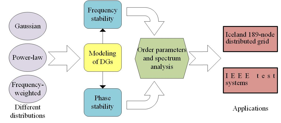
In practice, the error occurs in the installation process often obey Gaussian distribution, the weight distribution of complex network is mostly in line with the power-law distribution, and the frequency-weighted distribution can reflect some peculiarities of the actual network. Thus, this paper discusses the weighting methods of Gaussian distribution, power-law distribution, and frequency-weighted network, and the aforementioned methods can be simulated by adjusting the weight index.

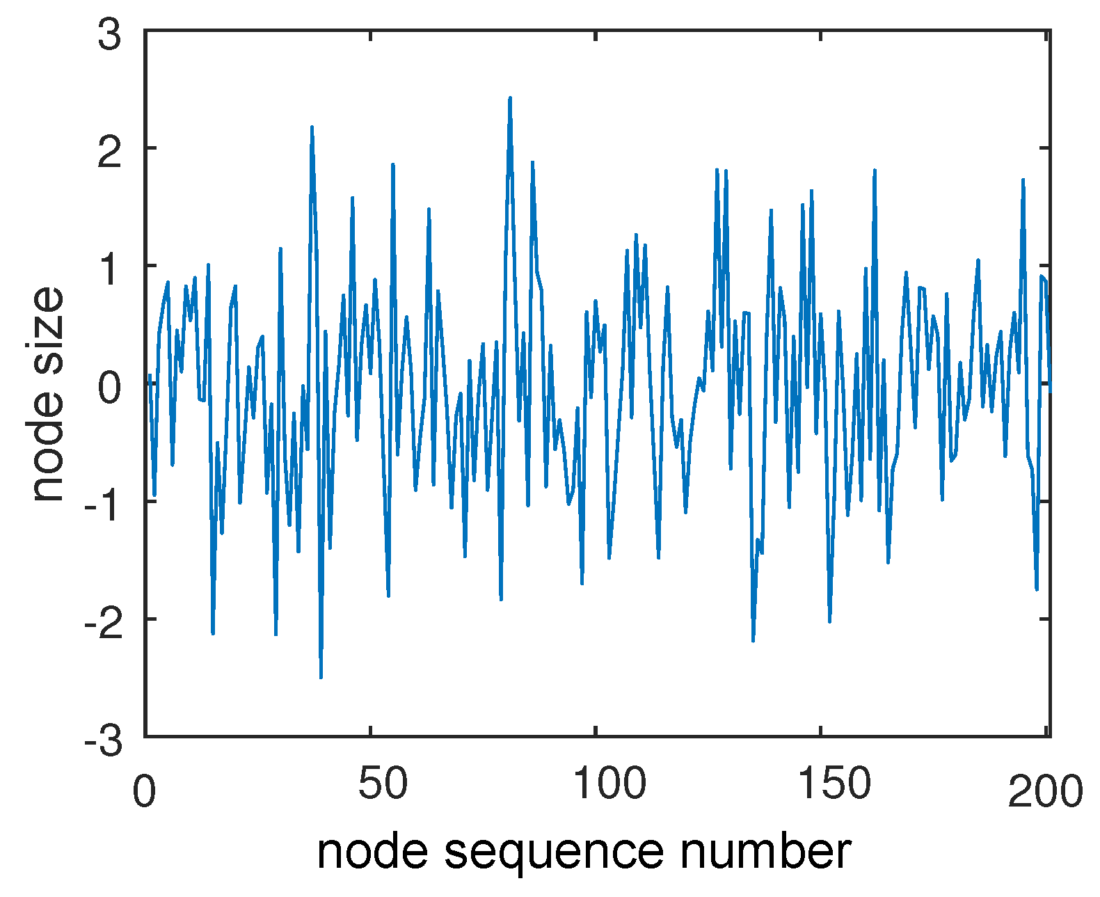
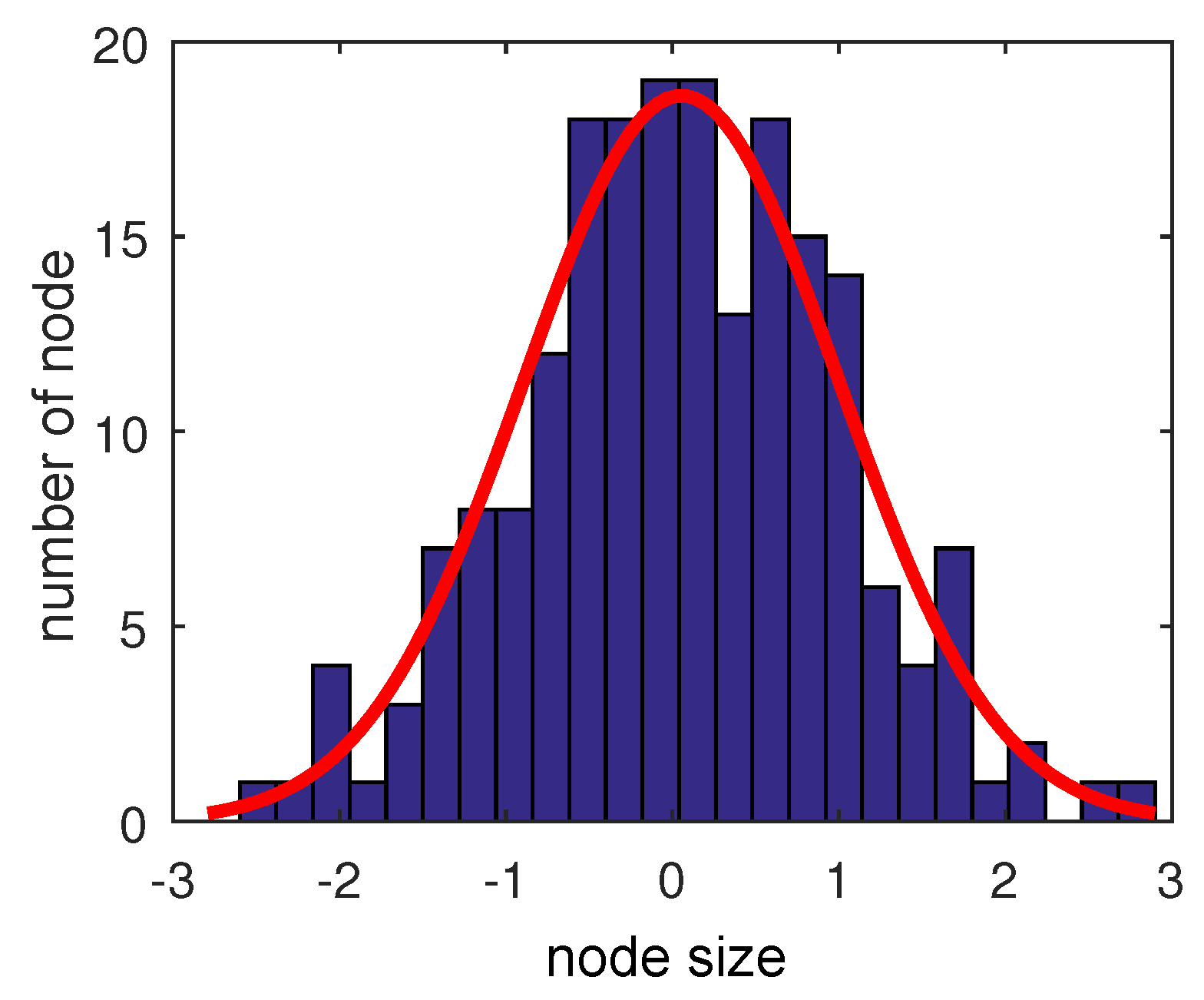
3.3.1. Gaussian Distribution

At first, this paper considers the case that the weight distribution method is the same as the rated frequency of an inverter distribution method so that the distribution function $g\left(m\right)$ of $m_i$ is the same as the distribution function $g\left(\omega \right)$ of ${\omega }_i$; both are Gaussian distribution. Unlike the rated frequency of the inverter being a symmetric normal distribution of 50, the weight distribution is a symmetric normal distribution of the y-axis. Its Kuramoto oscillator model is:

$$\begin{array}{c}{\dot{\theta }}_i={\omega }_i+kg\left(m\right){\displaystyle \sum _{j=1}^N}{a}_{ij}sin({\theta }_i-{\theta }_j),i=1,\dots ,N\hfill \\ ={\omega }_i+k\left|m_i\right|{\displaystyle \sum _{j=1}^N}{a}_{ij}sin({\theta }_i-{\theta }_j),i=1,\dots ,N.\hfill \end{array}$$

(14)

$a_{ij}=1$ when DG${}_i$ has coupling relationship with DG${}_j$, otherwise $a_{ij}=0$.

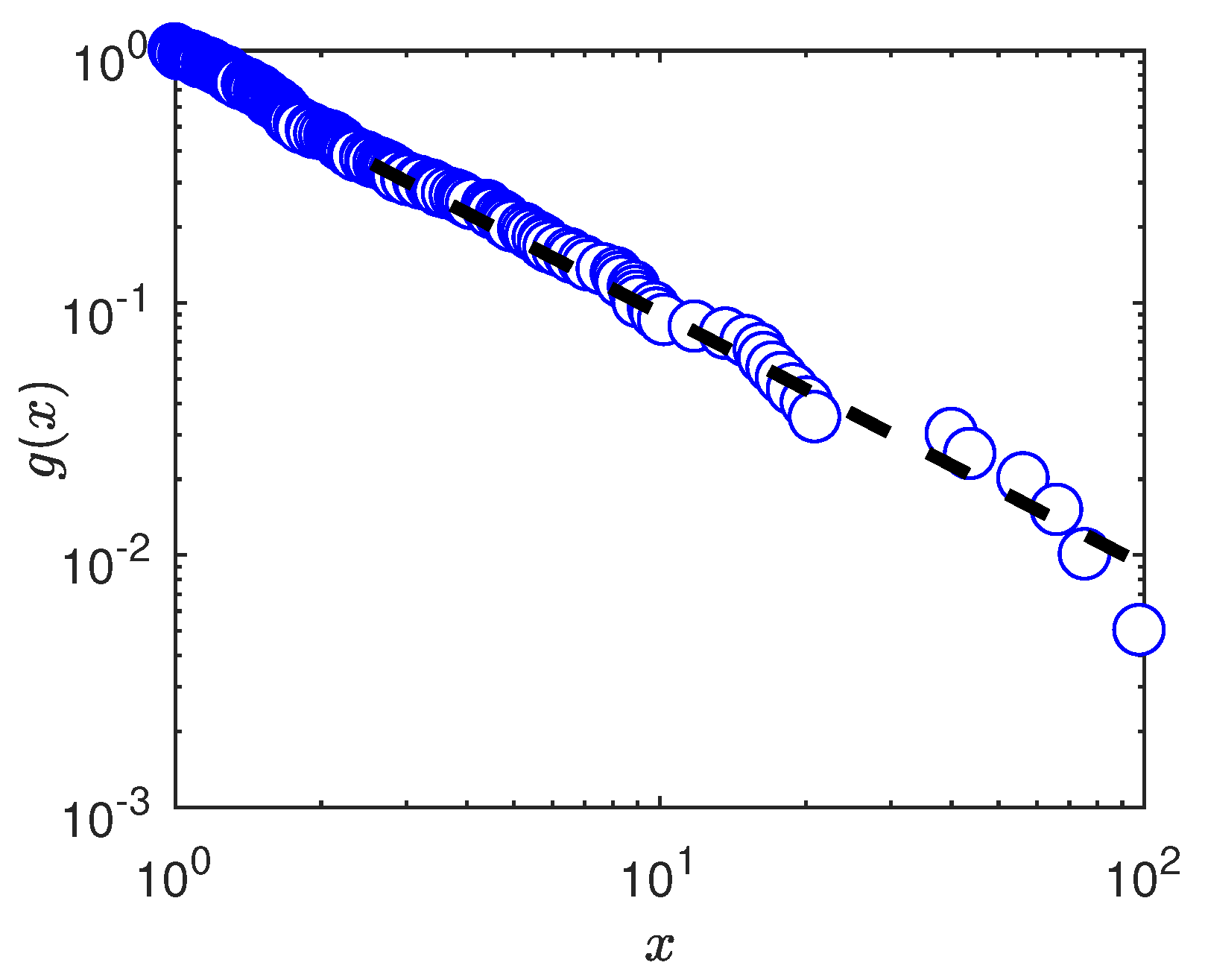
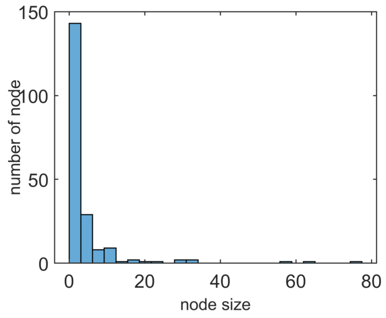
3.3.2. Power-Law Distribution

Power-law distribution has extensive application in complex network theory. Barabasi and Albert pointed out that the degree distribution of complex networks is the power-law distribution in [31]. Then, Chunguang Li and Guanrong Chen verified that the weight distribution is a power-law distribution in a general complex network. Furthermore, according to the research of Barrat et al. in [32], the node strength distribution in the weighted network obeys the power-law distribution as well. In this paper, only the weighted distribution of weights is discussed. Therefore, it is worth mentioning that the assumed distribution function $g\left(m\right)$ of $m_i$ satisfies the power-law distribution, which means $g\left(m\right)\sim m^{-\beta }$, and

$$\begin{array}{c}\dot{\theta }={\omega }_i+kg\left(m\right){\displaystyle \sum _{j=1}^N}{a}_{ij}sin({\theta }_i-{\theta }_j),i=1,\dots ,N\hfill \\ ={\omega }_i+k{m}_i{\displaystyle \sum _{j=1}^N}{a}_{ij}sin({\theta }_i-{\theta }_j),i=1,\dots ,N\hfill \end{array}$$

(15)

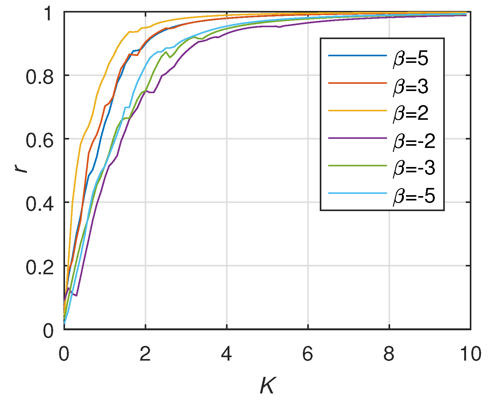
3.3.3. Frequency-Weighted Network

The frequency-weighted network reflects the feature of several natural and social networks. In fact, a power grid could be expressed as a Kuramoto oscillator model, and the weight of the coupling strengths are obtained by their natural frequency. In this case, the weighted coupling coefficients are related to DGs’ own inverter rated frequency rather than the topology of a network. We added the inverter rated frequency to the dynamic model as follows:

$${\dot{\theta }}_i={\omega }_i+\frac{k\left|{\omega }_i\right|}{{\sum }_{j=1}^N{a}_{ij}}\sum _{j=1}^N{a}_{ij}sin({\theta }_i-{\theta }_j),i=1,\dots ,N$$

(16)

3.4. Critical Coupling Strength Formula

Reference [23] pointed out that any fixed point in Equation (7) has local exponential stability when ${∥{\phi }^{\ast }∥}_{\infty }\le \pi /2$. For the sake of simplicity, we decompose the matrix $A=k\times A^{\prime }$, where $A^{\prime }$ is the adjacency matrix entirely determined by weight indexes, and k is the coupling strength. The in-degree matrix D is a diagonal matrix, whose values in each row are the row sum of corresponding rows of A matrix. Certainly, the D matrix can be decomposed into $D=k\times D^{\prime }$, where $D^{\prime }$ is the in-degree matrix entirely determined by weight indexes. At the same time, the Laplacian matrix $L=D-A$ can be decomposed into $L=k\times L^{\prime }$, where $L^{\prime }$ is the Laplacian matrix entirely determined by weight indexes. Furthermore, Equation (9) can be decomposed into:

$$sin\left({\phi }^{\ast }\right)=k^{-1}{B}^T{\left(L^{\prime }\right)}^{†}\omega$$

(17)

There is ${∥sin\left(B^T{\theta }^{\ast }\right)∥}_{\infty }=1$ when the network enters a critical stable state, and then the critical coupling values of star topology in different weighting methods can be transformed into the following formula:

$$k_c={∥B^T{\left(L^{\prime }\right)}^{†}\omega ∥}_{\infty }$$

(18)

The calculation of the critical coupling value in different weighting methods is described in detail in Section 4.

4. Simulation

In this section, three weighted methods from above are simulated, and the proposed formula of critical coupling (18) is verified.

4.1. Case 1

It is inevitable that deviations will generate in the process of installing the grid-tied DG inverters in an active distribution network, and the distribution of deviations often conforms to the Gaussian distribution.

In this case, the assumed actual parameters are reported in

Table 1. Related parameters in Case 1.

Type	Parameter
wire type	YJV-3
wire section	3 × 120 mm${}^2$
wire resistance	0.153/km
wire length	100 km
number of DG	51/101/201
wire type in inverter	YJV-4
wire section in inverter	4 × 16 mm${}^2$
wire resistance in inverter	1.15/km
wire length in inverter	10 km
rated frequency of inverter	50 Hz
distribution of inverter rated frequency	Gaussian distribution
distribution of weight index	Gaussian distribution
voltage classes	220 V

:

4.1.1. Weighted Undirected Network

Let us now turn to the case of the undirected situation, the weight distribution of edges in this situation conforms to the Gaussian distribution $X\sim N(0,1)$, and source point and sink point of each edge are arbitrary. When N takes 201, and the number of edges takes 200 in this case; meanwhile, the distribution is depicted in Figure 3. Furthermore, Figure 4 shows the probability density function of this Gaussian distribution, and it is obvious that the distribution law conforms to the (0,1) distribution.

Thus, the ordinary differential equation of oscillator ${\theta }_i$ is

$$\dot{\theta }={\omega }_i+kX\sum _{j=1}^N{a}_{ij}sin({\theta }_i-{\theta }_j),i=1,\dots ,N$$

(19)

where X is the weight of the corresponding edge.

Turn now to verifying the critical coupling strength formula of the weighted situation proposed in Section 3. In this case,

$$L={\left[\begin{array}{cccc}-{\displaystyle \sum _1^{200}}X& X_1& \cdots & X_{200}\\ X_1& -X_1& \cdots & 0\\ ⋮& ⋮& ⋮& ⋮\\ X_{200}& 0& \cdots & -X_{200}\end{array}\right]}_{(201\times 201)}$$

(20)

Furthermore, the related parameters in this case are depicted in Table 1, and the weight $k=\left|\frac{a}{Z+Z_{\mathrm{inv}}}\right|\times E^2=\frac{0.1\times {220}^2}{100\times 0.153+10\times 1.15}=180$. The phase and frequency stability are shown in Figure 5 and Figure 6, and it can be seen that the phases of DG nodes change at the same rate and the frequency of DG nodes fixed in one constant value.

In this paper, order parameters are used to reflect the synchronization of DGs in the network. Figure 7 shows the relationship between the coupling strength K and the order parameter r when N has different values, which reflect the change of network synchronization with the coupling strength. It is obvious that the network stability is the best when the value of N is 51, followed by 101. When N takes 201, the network has the worst stability. It can be seen that the stability of the network decreases with the increase of N, which is not consistent with the situation in which the stability does not change with the value of N when the star topology is an undirected network.

4.1.2. Weighted Directed Network

Thus far, this paper has focused on an ideal situation that the weighted distribution of the undirected edge in the network is Gaussian distribution. Let us now turn to consider the weighted directed case. In a power grid, each DG can become not only the power transmitter but also the power receiver. Therefore, it is of great practical value to consider the different weights of edges when they take different directions between coupling DG nodes. That is, the edge weight is the weight index of the master node when the master node is the source point, while the edge weight is the weight index of the load node when the load node is the source point:

Since the inverter rated frequency of the DG unit also conforms to the Gaussian distribution, this paper assumes that the weight distribution of edges is the same type as the distribution of inverter rated frequency. Namely, the ordinary differential equation with the oscillator ${\theta }_i$ is

$$\dot{\theta }={\omega }_i+k\left|{\omega }_i\right|\sum _{j=1}^N{a}_{ij}sin({\theta }_i-{\theta }_j),i=1,\dots ,N$$

(21)

This paper takes the weight index of the load node as the Gaussian distribution and the weight index of the master node as the mean value of the weight index of each load node to realize the power balance. Thus, there is

$$\begin{array}{c}L={\left[\begin{array}{cccc}(n-1)\ast m_1& m_1& \cdots & m_1\\ m_2& -m_2& \cdots & 0\\ ⋮& ⋮& ⋮& ⋮\\ m_n& 0& \cdots & -m_n\end{array}\right]}_{(201\times 201)}\hfill \\ ={\left[\begin{array}{cccc}-{\sum }_2^{201}{m}_i& \frac{{\sum }_2^{201}{m}_i}{200}& \cdots & \frac{{\sum }_2^{201}{m}_i}{200}\\ m_2& -m_2& \cdots & \cdots \\ ⋮& ⋮& ⋮& ⋮\\ m_n& 0& \cdots & -m_n\end{array}\right]}_{(201\times 201)}\hfill \end{array}$$

(22)

Frequency deviation will lead to power imbalance and even instability of the whole system. The phase and frequency stabilization processes in the directed situation are shown in Figure 8 and Figure 9 when k = 180. Obviously, the coupling strength k in this case is much greater than the critical coupling strength required for network stability. Let us now turn to the critical coupling strength in the case of Gaussian distribution. When N = 201, the value of L matrix can be substituted for formula (18) to obtain the critical coupling strength $K_C$ = 6.7; when N is 51 and 101, the critical coupling strength $K_C$ = 3.7 and 4.46 can be obtained from the calculation formula, respectively. Figure 10 shows that, when N takes 201, the network enters synchronization rapidly before $K<6.7$, while the network is nearly stable after $K>6.7$. This result is basically consistent with the result obtained by formula (4-1). Similarly, when the value of N is 51 and 101, the network becomes stable after $K_C$ = 3.7 and 4.46, respectively. Thus far, two conclusions have been shown. The first is that the validity of the critical coupling strength formula (18) in the directed weighted network is verified, and the second is that the network stability decreases with the increasing number of nodes in the island star topology directed weighted network.

4.2. Case 2

In particular, previous studies show that most of the nodes have a degree that is a less than average value while a few nodes have large connections in the real network. The study of Chunguang Li and Guanrong Chen [17] confirmed that the distribution of connection weights would follow the power-law distribution in general actual complex networks. Thus, it is important to research the stability of a weighting case that conforms to the power-law distribution.

In this case, the assumed actual parameters are reported in

Table 2. Related parameters in Case 2.

Type	Parameter
wire type	YJV-3
wire section	3 × 120 mm${}^2$
wire resistance	0.153/km
wire length	100 km
number of DG	51/101/201
wire type in inverter	YJV-4
wire section in inverter	4 × 16 mm${}^2$
wire resistance in inverter	1.15/km
wire length in inverter	10 km
rated frequency of inverter	50 Hz
distribution of inverter rated frequency	Gaussian distribution
distribution of weight index	Power-law distribution
voltage classes	220 V

:

4.2.1. Weighted Undirected Network

In this case, we assume that the weight distribution of 200 edges conforms to the power-law distribution, as shown in Figure 11. Then, Figure 12 shows the probability density function diagram. It can be seen that, with the increase of abscissa, the probability of weight distribution is lower. Furthermore, the probability of randomly selecting a node with greater weight is negatively correlated with the number of the same weight. The power-law index in Figure 11 is 2. The distribution of nodes depicted as a line whose slope is negative in the double logarithmic diagram, as demonstrated in Figure 12. This distribution has an asymptote of the black dotted line, where the exponent determines the rate of decay.

The weighted distribution in this case follows $g\left(X\right)\sim X^{-\beta }$, which means that the ordinary differential equation of oscillator ${\theta }_i$ is

$$\dot{\theta }={\omega }_i+kX\sum _{j=1}^N{a}_{ij}sin({\theta }_i-{\theta }_j),i=1,\dots ,N$$

(23)

where X is the weight of the corresponding edge.

Like the weighted undirected network in case 1, the weighted distribution in this case is reflected by the value of the edge weight, so the Laplace matrix is

$$L={\left[\begin{array}{cccc}-{\displaystyle \sum _1^{200}}X& X_1& \cdots & X_{200}\\ X_1& -X_1& \cdots & 0\\ ⋮& ⋮& ⋮& ⋮\\ X_{200}& 0& \cdots & -X_{200}\end{array}\right]}_{(201\times 201)}$$

(24)

The same as the coupling strength value of case 1, the phase and frequency stabilization process diagram are shown in Figure 13 and Figure 14. In addition, the influence of different power exponents on network stability is shown in Figure 15. Figure 15 shows the network synchronization process when power-law index $\beta$ grades –5, –3, –2, 2, 3, 5. It is obvious that the critical coupling strength of the system when the power-law index is positive does not differ greatly, while the positive power-law index values have significantly better stability than the negative values. This paper comes to a conclusion that the positive and negative value of power-law index rather than the size of the Power-law index has a key influence on the stability of the network when ignoring the deviations generated in the calculation process.

The simulation analysis of the different number of nodes N is shown in Figure 16. When the index is 2, the value of N is negatively correlated with network stability. The conclusion also reflects the analysis of the relationship between the node number and the network stability in the previous case.

4.2.2. Weighted Directed Network

Turn now to the directed weighted case. Similar to case 1, the method of adjusting the weight index is used to complete the weight distribution conforms to the power-law distribution $g\left(m\right)\sim m^{-\beta }$, and the ordinary differential equation is given in the formula (25):

$$\dot{\theta }={\omega }_i+kg\left(m\right)\sum _{j=1}^N{A}_{ij}sin({\theta }_i-{\theta }_j),i=1,\dots ,N$$

(25)

Similar to the weighted directed network in case 1, the weight index of the master node in this case is the mean value of the weight index of each load node considering the problem of power balance. Therefore, the Laplace matrix in the network with 201 nodes is:

$$\begin{array}{c}L={\left[\begin{array}{cccc}(n-1)\ast m_1& m_1& \cdots & m_1\\ m_2& -m_2& \cdots & 0\\ ⋮& ⋮& ⋮& ⋮\\ m_n& 0& \cdots & -m_n\end{array}\right]}_{(201\times 201)}\hfill \\ ={\left[\begin{array}{cccc}-{\sum }_2^{201}{m}_i& \frac{{\sum }_2^{201}{m}_i}{200}& \cdots & \frac{{\sum }_2^{201}{m}_i}{200}\\ m_2& -m_2& \cdots & \cdots \\ ⋮& ⋮& ⋮& ⋮\\ m_n& 0& \cdots & -m_n\end{array}\right]}_{(201\times 201)}\hfill \end{array}$$

(26)

The phase and frequency stabilization process in the directed situation are shown in Figure 17 and Figure 18 when the value of power-law index beta is 2, and coupling strength k is 180. When the value of the power-law index respectively takes –5, –3, –2, 2, 3, 5, the critical coupling strength $K_C$ of network is respectively 1.4976, 1.4353, 1.9639, 1.4976, 1.4353, and 0.7771 by formula (18). These critical coupling strengths are nearly consistent with the critical value depicted in Figure 19. In addition, the weighted directed network has similar performance to the weighted undirected network, which means that the positive power-law index value has better network stability performance than the negative one, while the size of the power-law index value has almost no effect. Apparently, in the case of power-law distribution, the stability of the network is obviously better than that in the case of Gaussian distribution. When the Power-law index is 2, the network can be stable only on the condition that the coupling strength is greater than the critical value $K_C$ = 0.5475.

Furthermore, the relationship between the number of DG nodes and network stability is shown in Figure 20. The negative correlation between DG number and critical coupling strength is still evident.

4.3. Case 3

The following case will discuss the Frequency-weighted situation. The natural frequency is inverter rated frequency in the Kuramoto oscillator model. Thus, case 3 chooses the absolute ratio between the inverter rated frequency of one DG node and its in-degree as the weight; there is the ordinary differential equation:

$$\dot{\theta }={\omega }_i+\frac{k\left|{\omega }_i\right|}{{\sum }_{j=1}^N{A}_{ij}}\sum _{j=1}^N{A}_{ij}sin({\theta }_i-{\theta }_j),i=1,\dots ,N$$

(27)

The weighted distribution in this case is different from the previous two cases, whose weight index is not a random value which obeys a certain distribution. The Laplace matrix in this case is

$$L={\left[\begin{array}{cccc}-\left|{\omega }_1\right|& \frac{\left|{\omega }_1\right|}{200}& \cdots & \frac{\left|{\omega }_1\right|}{200}\\ \left|{\omega }_2\right|& -\left|{\omega }_2\right|& 0& 0\\ ⋮& ⋮& ⋮& ⋮\\ \left|{\omega }_{n-1}\right|& 0& \cdots & 0\\ \left|{\omega }_n\right|& 0& \cdots & -\left|{\omega }_n\right|\end{array}\right]}_{(201\times 201)}$$

(28)

In case 3, the phase and frequency stabilization process diagram are shown in Figure 21 and Figure 22, which are similar to the above two cases. According to formula (18), the critical coupling strength of this case is $K_C$ = 12.89 when N = 201, and the network synchronization progress is shown in Figure 23. It can be seen that the weighted method in this case is not as stable as the Gaussian distribution and the power-law distribution.

4.4. Stability Analysis

Through comparing the critical coupling strength of three cases as illustrated in Figure 24, we find that the power-law distribution has the best stability in different weighted distribution methods. Moreover, the second largest eigenvalue ${\lambda }_2$ or the eigenvalue proportion ${\lambda }_N/{\lambda }_2$ in adjacency matrix A could describe the synchronization ability of the system. The network coherence is proportional to ${\lambda }_2$ and inversely proportional to ${\lambda }_N/{\lambda }_2$.

Table 3. Spectrum analysis.

Distribution Mode	${\mathit{\lambda }}_2$	${\mathit{\lambda }}_{\mathit{N}}$	${\mathit{\lambda }}_{\mathit{N}}/{\mathit{\lambda }}_2$
Gaussian distribution	–1.005	–557.16	554.38
Power-law distribution	–1.006	–436.59	433.98
Frequency-weighted	–1.0007	–686.99	686.51

shows that the ${\lambda }_2$ of power-law distribution has the smallest value, which means it has the best synchronization ability, followed by the Gaussian distribution and frequency-weighted distribution. Thus, the results of Table 3 and Figure 24 confirm each other. In addition, the contrastive analysis of weighted directed network and weighted undirected network show that the weighted directed network which conforms to the Gaussian distribution or power-law distribution is easier to get into synchronization than the weighted undirected network. Furthermore, by studying the network with different numbers of DG, this paper finds that the stability of the weighted network decreases with an increase of N, which is different from the average field. For the weighting method of power-law distribution, the size of the power-law index $\beta$ is not significant to the stability of the network, but the sign of the power-law index $\beta$ is not negligible to the stability of the network.

4.5. Further Analysis of Weighted Network in the Actually Distributed Network

Actually, the topology structure of an actual power grid network often isn’t a standard star topology. The standard star topology is an ideal assumption. In order to verify the stability analysis from the above subsection, we take the dynamic IEEE test systems [33] and the Iceland 189-node distributed grid [34] as a research object. The synchronizing processes of Gaussian distribution, power-law distribution, and frequency-weighted network are shown in Figure 25 and Figure 26.

4.5.1. Dynamic IEEE Test Systems

Three different weighted distribution methods have been applied to the dynamic IEEE models, including 9-bus, 14-bus, 57-bus, and 118-bus modified test systems. The diagram of coupling strength and order parameter is shown in Figure 25, where the labels G, P, and F represent Gaussian distribution, Power-law distribution and frequency-weighted distribution, respectively, and the network with the Power-law distribution method always enter the stable state at first. The value of the critical coupling strength of three weighted distribution methods in the dynamic IEEE test systems is shown in

Table 4. $K_c$ of three weighted distribution methods in different IEEE systems.

IEEE Test Systems	9-bus	14-bus	57-bus	118-bus
Gaussian distribution	3.4	4.2	47	56.1
Power-law distribution	1.1	1.5	10.7	16.1
Frequency-weighted	4.5	4.9	78.4	113.4

, where each value is calculated by Equation (18). It shows that the network with the power-law distribution method always has the least critical coupling strengths, which corresponds to the stability performance in Figure 25.

4.5.2. Iceland 189-Nodes Distribution Grid

Figure 26 shows the results of the stability performance of three distribution methods in an Iceland 189-nodes distribution grid. It can be seen that the power-law distribution undoubtedly has the best stability performance. Second is the frequency-weighted network. Moreover, the Gaussian distribution needs a long process to enter synchronization. These results further support the conclusions of the above subsection.

5. Conclusions

Above all, this paper analyzes the stability of large-scale grid-tied DG in a non-homogeneous active power network by using complex networks theory.

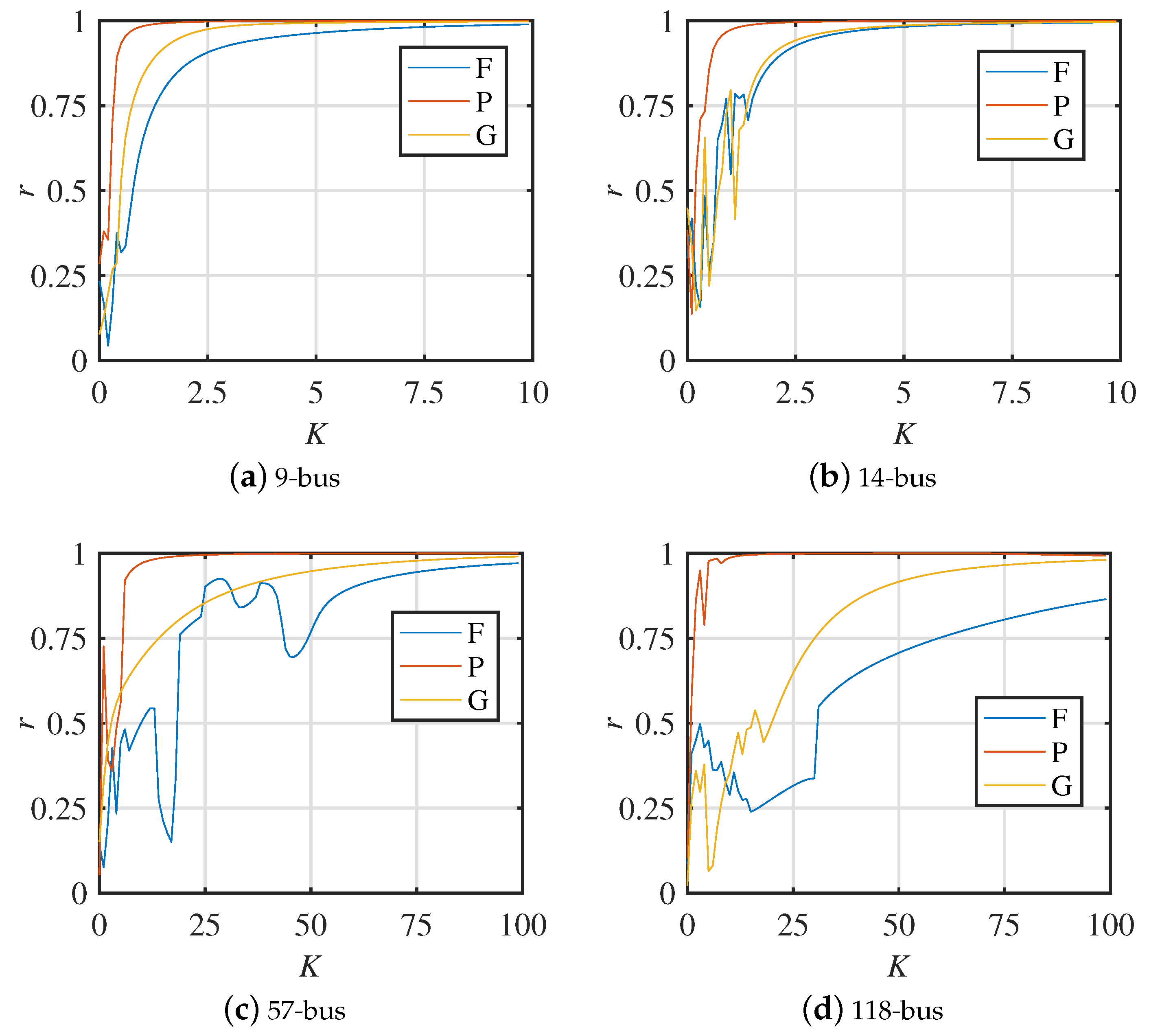
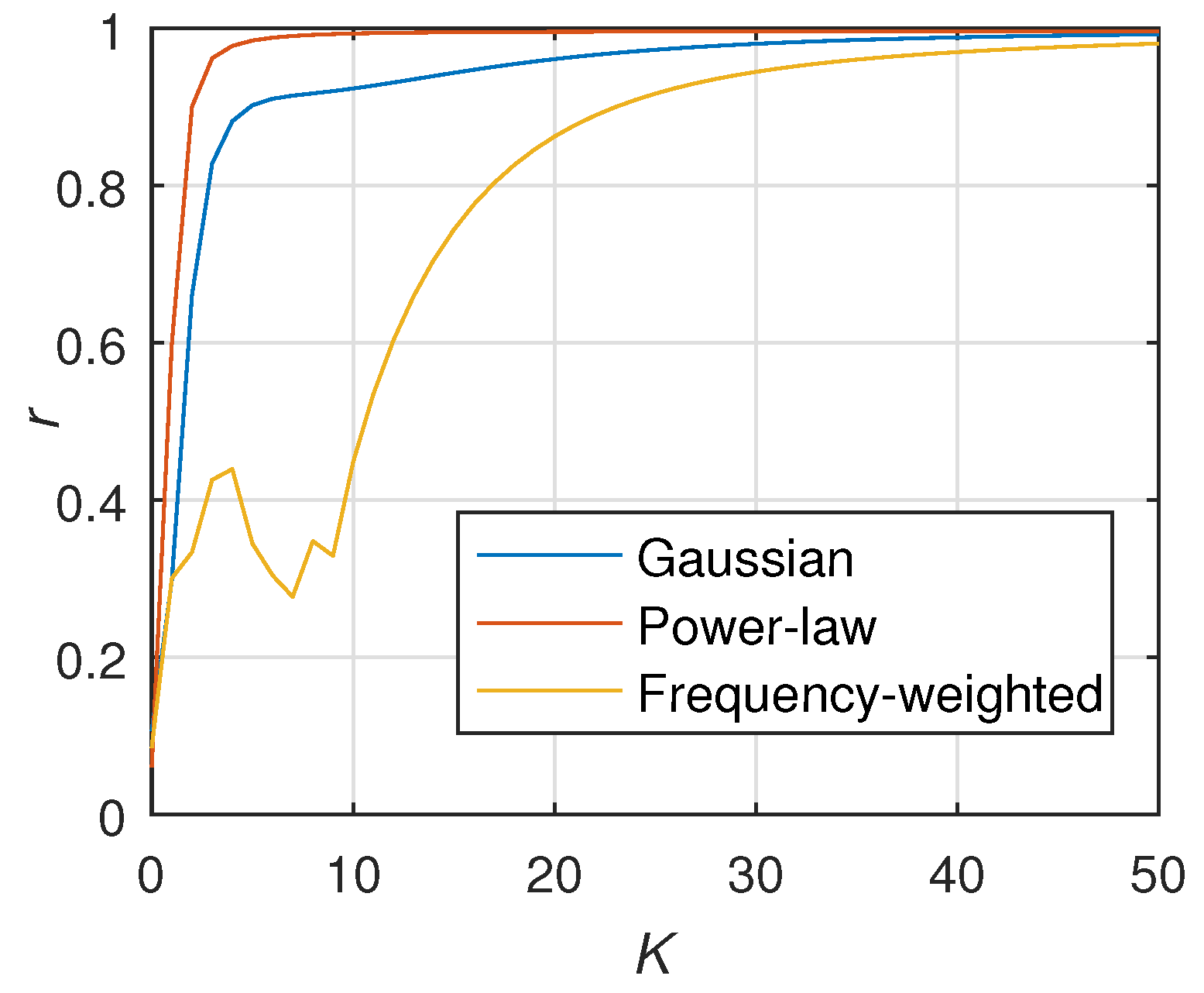
Then, three different weighting distribution methods, including Gaussian distribution, power-law distribution, and frequency-weighted distribution, are analyzed. In addition, the critical coupling strength formula for the weighted situation $k_c={∥B^T{\left(L\right)}^{†}\omega ∥}_{\infty }$ has been proposed and verified. The critical coupling strength obtained from this formula conforms to the reality when ignoring tiny deviation.

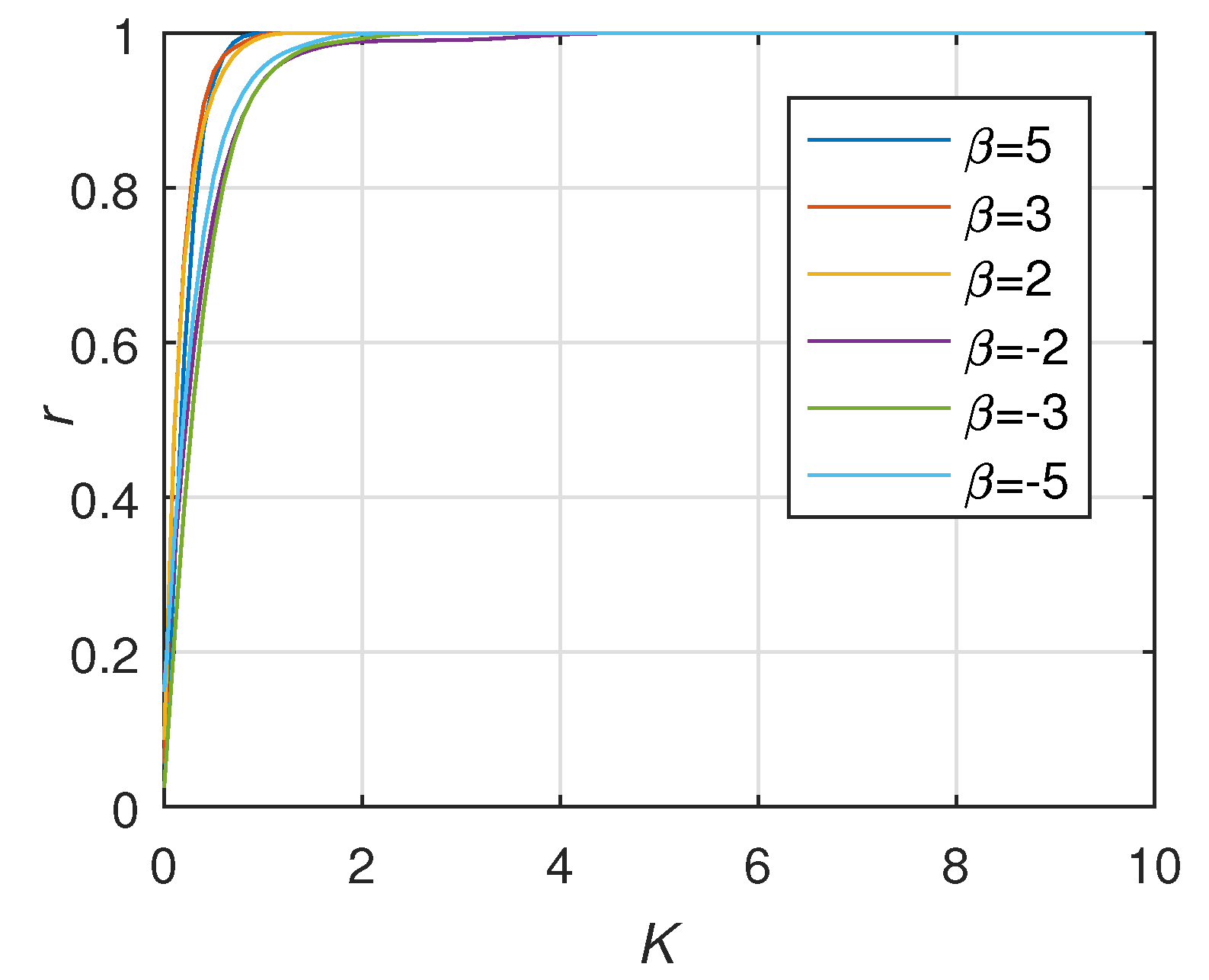
Among the three different weighting methods, the power-law distribution has the best stability. Moreover, the difference of power-law index value has little effect on the network stability, but the sign of power-law index has quite an effect on the system stability. The second is the Gaussian distribution, which is obviously less stable than the power-law distribution. Finally, the frequency-weighted network has the worst synchronization performance, which is significantly inferior to the other two. In addition, further analysis of the IEEE dynamic test systems and the Iceland 189-node distributed grid has proved the better stability of power-law distribution in this paper.

References

1. Uriarte, F.M.; Smith, C.; VanBroekhoven, S.; Hebner, R.E. Microgrid ramp rates and the inertial stability margin. IEEE Trans. Power Syst. 2015, 30, 3209–3216. [Google Scholar] [CrossRef]
2. Mendis, N.; Muttaqi, K.M.; Perera, S. Management of battery-supercapacitor hybrid energy storage and synchronous condenser for isolated operation of PMSG based variable-speed wind turbine generating systems. IEEE Trans. Smart Grid 2014, 5, 944–953. [Google Scholar] [CrossRef]
3. Lai, J.; Lu, X.; Yu, X.; Monti, A. Cluster-Oriented Distributed Cooperative Control for Multiple AC Microgrids. IEEE Trans. Ind. Inform. 2019, 15, 5906–5918. [Google Scholar] [CrossRef]
4. Lai, J.; Lu, X.; Yu, X.; Monti, A. Stochastic Distributed Secondary Control for AC Microgrids via Event-Triggered Communication. IEEE Trans. Smart Grid 2020. to be published. [Google Scholar] [CrossRef]
5. Lai, J.; Lu, X.; Yu, X.; Monti, A.; Zhou, H. Distributed Voltage Regulation for Cyber-Physical Microgrids with Coupling Delays and Slow Switching Topologies. IEEE Trans. Syst. Man Cybernet. Syst. 2020, 50, 100–110. [Google Scholar] [CrossRef]
6. Lai, J.; Lu, X. Nonlinear Mean-Square Power Sharing Control for AC Microgrids under Distributed Event Detection. IEEE Trans. Ind. Inform. 2020. to be published. [Google Scholar] [CrossRef]
7. Refaat, S.S.; Abu-Rub, H.; Sanfilippo, A.P.; Mohamed, A. Impact of grid-tied large-scale photovoltaic system on dynamic voltage stability of electric power grids. IET Renew. Power Gener. 2018, 12, 157–164. [Google Scholar] [CrossRef]
8. Byshkin, M.; Stivala, A.; Mira, A.; Robins, G.; Lomi, A. Fast Maximum Likelihood estimation via Equilibrium Expectation for Large Network Data. Nature 2013, 31, 1. [Google Scholar] [CrossRef]
9. Brockmann, D.; Helbing, D. The Hidden Geometry of Complex, Network-Driven Contagion Phenomena. Science 2013, 342, 1337–1342. [Google Scholar] [CrossRef] [Green Version]
10. Centola, D. The Spread of Behavior in an Online Social Network Experiment. Science 2010, 329, 1194–1197. [Google Scholar] [CrossRef]
11. Li, X. The role of degree-weighted couplings in the synchronous onset of Kuramoto oscillator networks. Physica A Stat. Mech. Its Appl. 2008, 387, 6624–6630. [Google Scholar] [CrossRef]
12. Wu, C.W. Synchronizability of networks of chaotic systems coupled via a graph with a prescribed degree sequence. Phys. Lett. A 2005, 346, 281–287. [Google Scholar] [CrossRef]
13. Sorrentino, F.; di Bernardo, M.; Garofalo, F. Synchronizability In addition, Synchronization Dynamics Of Weighed And Unweighed Scale Free Networks With Degree Mixing. Int. J. Bifurc. Chaos 2007, 17, 2419–2434. [Google Scholar] [CrossRef] [Green Version]
14. Leyva, I.; Sendinanadal, I.; Almendral, J.A. Explosive synchronization in weighted complex networks. Phys. Rev. E Stat. Nonlinear Soft Matter Phys. 2013, 88, 042808. [Google Scholar] [CrossRef] [Green Version]
15. Zhu, L.; Tian, L.; Zhu, C.; Shi, D. Effects of coupling-frequency correlations on synchronization of complete graphs. Phys. Lett. A 2013, 377, 2749–2753. [Google Scholar] [CrossRef]
16. Chavez, M.; Hwang, D.U.; Amann, A. Synchronization is enhanced in weighted complex networks. Phys. Rev. Lett. 2005, 94, 218701. [Google Scholar] [CrossRef]
17. Jalili, M.; Mazloomian, A. Weighted coupling for geographical networks: Application to reducing consensus time in sensor networks. Phys. Lett. A 2010, 374, 3920–3925. [Google Scholar] [CrossRef]
18. Qin, B.Z.; Lu, X.B. Adaptive approach to global synchronization of directed networks with fast switching topologies. Phys. Lett. A 2010, 374, 3942–3950. [Google Scholar] [CrossRef]
19. Dong, Z.; Tian, M.; Lu, Y.; Lai, J.; Tang, R.; Li, X. Impact of core-periphery structure on cascading failures in interdependent scale-free networks. Phys. Lett. A 2019, 383, 607–616. [Google Scholar] [CrossRef]
20. Tian, M.; Dong, Z.; Cui, M.; Wang, J.; Wang, X.; Zhao, L. Energy-supported cascading failure model on interdependent networks considering control nodes. Physica A Stat. Mech. Its Appl. 2019, 522, 195–204. [Google Scholar] [CrossRef]
21. Dorfler, F.; Chertkov, M.; Bullo, F. Synchronization in complex oscillator networks and smart grids. Proc. Natl. Acad. Sci. USA 2013, 110, 2005–2010. [Google Scholar] [CrossRef] [PubMed] [Green Version]
22. Bidram, A.; Davoudi, A.; Lewis, F.L.; Nasirian, V. Cooperative Synchronization in Distributed Microgrid Control; Springer: Cham, Switzerland, 2017. [Google Scholar]
23. Fazlyab, M.; Dorfler, F.; Preciado, V.M. Optimal Design for Synchronization of Kuramoto Oscillators in Tree Networks. Physics 2005, 92, 181–189. [Google Scholar]
24. Gu, Y.Q.; Shao, C.; Fu, X.C. Complete synchronization and stability of star-shaped complex networks. Chaos Solitons Fractals 2006, 28, 480–488. [Google Scholar] [CrossRef]
25. Dekker, A.H.; Taylor, R. Synchronisation Properties of Trees in the Kuramoto Model. Siam J. Appl. Dynam. Syst. 2012, 12, 97–100. [Google Scholar]
26. Zhai, M. Transmission characteristics of low-voltage distribution networks in china under the smart grids environment. IEEE Trans. Power Deliv. 2011, 26, 173–180. [Google Scholar] [CrossRef]
27. Dorfler, F.; Bullo, F. Synchronization in complex networks of phase oscillators: A survey. Automatica 2014, 50, 1539–1564. [Google Scholar] [CrossRef] [Green Version]
28. Simpson-Porco, J.; Dorfler, F.; Bullo, F. Synchronization and power sharing for droop-controlled inverters in islanded microgrids. Automatica 2013, 49, 2603–2611. [Google Scholar] [CrossRef] [Green Version]
29. Pagani, G.; Aiello, M. Towards decentralization: A topological investigation of the medium and low voltage grids. IEEE Trans. Smart Grid 2011, 2, 538–547. [Google Scholar] [CrossRef]
30. Wu, Y.; Lee, C.; Liu, L. Study of reconfiguration for the distribution system with distributed generators. IEEE Trans. Power Deliv. 2010, 25, 1678–1685. [Google Scholar] [CrossRef]
31. Li, C.; Chen, G. Network connection strengths: Another power-law? arXiv 2003, arXiv:cond-mat/0311333. [Google Scholar]
32. Barrat, A.; Barth, M.; Pastorsatorras, R. The architecture of complex weighted networks. Proc. Natl. Acad. Sci. USA 2004, 101, 3747–3752. [Google Scholar] [CrossRef] [PubMed] [Green Version]
33. Dynamic IEEE Test Systems. 2019. Available online: https://www.kios.ucy.ac.cy/testsystems/index.php/dynamic-ieee-test-systems (accessed on 13 October 2019).
34. Power Systems Test Case Archive. 2013. Available online: http://www.maths.ed.ac.uk/optenergy/NetworkData/iceland/ (accessed on 13 October 2019).
Figure 1. Star topology.
Energies 13 01257 g001
Figure 2. Star topology electrical diagram.
Energies 13 01257 g002
Figure 3. Nodes in Gaussian distribution.
Energies 13 01257 g003
Figure 4. Probability density function of Gaussian distribution.
Energies 13 01257 g004
Figure 5. Phase stabilization process of undirected network in case 1.
Energies 13 01257 g005
Figure 6. Frequency stabilization process of undirected network in case 1.
Energies 13 01257 g006
Figure 7. The stability of the weighted undirected network when N is 51,101,201.
Energies 13 01257 g007
Figure 8. Phase stabilization process of directed network in case 1.
Energies 13 01257 g008
Figure 9. Frequency stabilization process of directed network in case 1.
Energies 13 01257 g009
Figure 10. The stability of the weighted directed network when N is 51,101,201.
Energies 13 01257 g010
Figure 11. Nodes in power-law distribution.
Energies 13 01257 g011
Figure 12. Probability density function of power-law distribution.
Energies 13 01257 g012
Figure 13. Phase stabilization process of undirected network in case 2.
Energies 13 01257 g013
Figure 14. Frequency stabilization process of undirected network in case 2.
Energies 13 01257 g014
Figure 15. The stability of the weighted undirected network when β is ± 2 , ± 3 , ± 5 .
Energies 13 01257 g015
Figure 16. The stability of the weighted undirected network when N is 51,101,201( β = 2 ).
Energies 13 01257 g016
Figure 17. Phase stabilization process of directed network in case 2.
Energies 13 01257 g017
Figure 18. Frequency stabilization process of directed network in case 2.
Energies 13 01257 g018
Figure 19. The stability of the weighted directed network when β is ± 2 , ± 3 , ± 5 ).
Energies 13 01257 g019
Figure 20. The stability of the weighted directed network when N is 51,101,201 ( β = 2 ).
Energies 13 01257 g020
Figure 21. Phase stabilization process in case 3.
Energies 13 01257 g021
Figure 22. Frequency stabilization process in case 3.
Energies 13 01257 g022
Figure 23. Synchronization progress when N is 51,101,201 in case 3.
Energies 13 01257 g023
Figure 24. Synchronization progress of different weighting distributions.
Energies 13 01257 g024
Figure 25. Synchronization progress of different weighting methods in the dynamic IEEE test systems.
Energies 13 01257 g025
Figure 26. Synchronization progress of different weighting methods in the Iceland 189-node distributed grid.
Energies 13 01257 g026