An Analytical Solution for Transient Productivity Prediction of Multi-Fractured Horizontal Wells in Tight Gas Reservoirs Considering Nonlinear Porous Flow Mechanisms

Abstract

Multi-fractured horizontal wells (MFHW) is one of the most effective technologies to develop tight gas reservoirs. The gas seepage from tight formations in MFHW can be divided into three stages: early stage with high productivity, transitional stage with declined productivity, and final stage with stable productivity. Considering the characteristics and mechanisms of porous flows in different regions and at different stages, we derive three coupled equations, namely the equations of porous flow from matrix to fracture, from fracture to near wellbore region, and from new wellbore region to wellbore then an unstable productivity prediction model for a MFHW in a tight gas reservoir is well established. Then, the reliability of this new model, which considers the multi-fracture interference, is verified using a commercial simulator (CMG). Finally, using this transient productivity prediction model, the sensitivity of horizontal well’s productivity to several relevant factors is analyzed. The results illustrate that threshold pressure gradient has the most significant influence on well productivity, followed by stress sensitivity, turbulence flow, and slippage flow. To summarize, the proposed model has demonstrated a potential practical usage to predict the productivity of multi-stage fractured horizontal wells and to analyze the effects of certain factors on gas production in tight gas reservoirs.

1. Introduction

Natural gas is an indispensable energy resource which plays an important role on the world’s energy map. As global demand continues to increase, conventional sources of natural gas will not be able to meet the world’s requirements. Consequently, the oil industry has shifted its research focus from conventional gas to unconventional natural gas, especially tight gas. Recently, alongside continuous developments in petroleum geology and the boost to oil and gas industry technologies, the exploitation and development of tight gas reservoirs has made considerable breakthrough and become the primary growth point for oil and gas production [1,2,3,4,5,6]. Because of its strong heterogeneity, complicated microscopic pore structure, and poor connectivity of the effective sand bodies, the porous flow mechanism of tight gas reservoirs is obviously distinct from those of conventional reservoirs. Moreover, because of poor reservoir physical properties, small discharging radius, lack of or low natural productivity, high development difficulty, and some other potential disadvantages, a MFHW with hydraulic stimulations is extensively used for developing tight gas reservoirs [7,8,9,10,11,12,13,14,15,16].

To date, many scholars are dedicated to the transient productivity of fractured wells in unconventional hydrocarbon reservoirs, considering the different characteristics of nonlinear flows compared to multi-scale flows. The methods to calculate the transient productivity of fractured horizontal wells primarily include analytical and numerical solutions, among which the analytical solution includes the complex potential theory, conformal transformation, and the equivalent flow resistance method [14,17,18]. Research on the transient productivity of tight gas reservoirs is increasingly wide. Through an iterative algorithm, Zheng et al. [19] quantified the correlation between saturation and pressure of the infinitesimal coal. They used the Corey relative permeability model to describe relative gas/water permeability as a function of the pressure. By applying the inter-porosity flow equation based on a pseudo-pressure, Zhenzihao et al. [20] developed a density-based rate-transient analysis technique, using which they predicted the gas production rate and were able to assess initial gas content in the system. This methodology is also capable of accurately forecasting gas production rates by converting the response of the corresponding liquid (separating pressure-dependent effects), which was performed using dimensionless depletion-driven parameters. Feng et al. [21] also developed a model thoroughly analyzing MFHWs in heterogeneous gas reservoirs. For this purpose, they used source functions, Green’s solution, and the element method to constrain a model in Laplace coordinates. However, by combining the pseudo-function method and material balance to describe homogeneous gas reservoirs, one cannot eliminate the nonlinearity of non-homogeneous gas reservoirs. To solve this issue, they calculated material balance by taking into account heterogeneous gas reservoirs from different regions. Jie et al. [22] created a new analytical model, which considers fracture damage and complex gas transport mechanisms as well as the shale gas stimulated reservoir volume (SRV). Berawala et al. [23] presented a mathematical 1D + 1D model to investigate the main controlling factors during a continuum-flow regime in shale-gas production in the context of well-induced fractures. Wenxi et al. [24] simulated shale gas production using a multi-stage fractured horizontal well using another model established in their study, which was based on a trilinear flow and did not assume that the secondary fracture length was equal to half the distance between hydraulic fractures. Jinzhou et al. [9] calculated gas productivity for the multi-staged horizontal wells in fractured tight sandstone gas reservoirs using a semi-analytical mathematical approach. Their model considered how flow in the fracture network (natural fracture system) affected the outcome. This helped to create a production forecast model of complex hydraulics with simulated impacts arising from natural fractures. As a result, after using the Gaussian elimination method, they obtained a semi-analytical solution.

Most previous studies simplified the nonlinear flow mechanisms of tight reservoirs to some extent. It is difficult to accurately and comprehensively reflect the actual flow state of fluid flowing into horizontal wells. To fill this gap, considering the seepage properties of the tight gas reservoirs and the steady-state seepage of fractured horizontal wells, we introduce the transient model of a matrix gas discharge radius. Considering the influence of various factors of tight reservoirs on the productivity, we also introduce the equivalent well diameter model. Under the same conditions, the pressure distribution equation of a single fracture is equivalent to the vertical well pressure distribution equation. Moreover, the transient productivity model describing a multi-stage fractured horizontal well is obtained. The actual data from a gas field in China were applied to verify the productivity model. It was demonstrated that two results obtained by the method proposed in this paper and dominant commercial software have an error of less than 1.62%, and the single parameter sensitivity analysis was also carried out. This paper provides a useful and feasible tool for reservoir engineers to predict, evaluate, and optimize the productivity of multi-fractured horizontal wells in tight gas reservoirs.

2. Reservoir Characteristics Analysis and Physical Model Assumptions

2.1. Productivity Forecast Model for Individual Horizontal Wells

As shown in Figure 1, for fractured horizontal wells, different production stages occur in different seepage areas within different flow media. Within the control area of individual wells, gas located in the fracture first flows to the wellbore. Next, the matrix near the wellbore area re-supplies the fracture. Therefore, the gas in the matrix flows toward the wellbore through the fracture. Then, the matrix far from the wellbore area supplies the matrix near the wellbore, and gas in the far wellbore area flows to the fracture through the matrix throat near the wellbore.

To achieve an accurate productivity prediction, based on the characteristics of different production stages of fractured horizontal wells in tight gas reservoirs, different flow media in each seepage area, and different seepage mechanisms, it is therefore necessary to establish corresponding productivity equations by considering the influence of factors such as: (a) threshold pressure gradient; (b) stress sensitivity effect; (c) slippage effect; and (d) high-speed non-Darcy effect. This comprehensive model is able to predict the productivity of the fractured horizontal wells accurately.

In the initial high-production stage, the artificial fractures are the primary flow medium, and hence the gas seepage occurs primarily in the artificial fractures. During this stage, the high-speed non-Darcy seepage cannot be ignored. Moreover, both stress-sensitive effects in artificial fractures and slippage effects play important roles. In the transition period, the gas seepage area is primarily in the proximity of the wellbore (SRV) and the flow medium is the matrix near the wellbore. In this stage, low-speed non-Darcy seepage plays a significant role, which is primarily affected by the threshold pressure gradient and the stress sensitive effect in the matrix. In the final stage of production, the seepage area is far from the wellbore (outside the SRV), and the flow medium is primarily the matrix far from the wellbore. In this stage, low-speed non-Darcy seepage plays a predominant role. However, the influence of the threshold pressure gradient, slippage effect, and stress sensitive effect in the matrix should be considered as well.

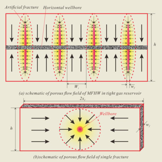
2.2. Physical Model Assumption

As shown in Figure 2, a fractured horizontal well with perforation completion is bored in a horizontal, infinite, homogeneous, and equal thickness tight gas reservoir. Some basic assumptions made for multi-stage fractured horizontal wells are as follows:

(1)

This model is applicable for isothermal single-phase unstable flows and the influence of gravity is neglected.

(2)

Fractures completely penetrate the target zone. Fractures and wellbores are arranged both symmetrically and equidistantly, and the fractures are perpendicular to the horizontal wellbore.

(3)

Gas flows evenly into fracture along the fracture wall and then into the horizontal wellbore through the fracture.

(4)

Mutual interference exists between the fractures and the pressure loss in the wellbore is neglected.

(5)

Contamination of the fracture wall is neglected.

(6)

Pressure loss in the horizontal wellbore is neglected.

3. Mathematical Model

3.1. Mathematical Model for Nonlinear Flow Mechanisms

Considering the threshold pressure gradient, stress sensitive effect, and slippage effect, the nonlinear flow mathematical model of tight gas reservoirs can be derived through the generalized form of Darcy’s Law [25,26].

3.1.1. Threshold Pressure Gradient Effect

Because of the differences of porosity structure characteristics, when gas receive the effect of surface molecules force, this will in turn contribute to the threshold pressure phenomena. Consequently, gas flow in low tight gas reservoirs obviously differs from that in conventional gas reservoirs with medium or high permeability [27]. The threshold pressure gradient, which is associated with non-Darcy flow in low-permeability reservoirs, is defined as the level of pressure gradient that must be attained to enable the fluid to flow.

$$v_{\mathrm{g}}=\frac{K_{\mathrm{g}}}{{\mu }_{\mathrm{g}}}(\frac{dp}{d\overline{y}}-\lambda )$$

(1)

where $v_{\mathrm{g}}$ is velocity of gas, m/s; $K_{\mathrm{g}}$ is permeability measured by gas, mD; ${\mu }_{\mathrm{g}}$ is gas viscosity, $\mathrm{mPa}·\mathrm{s}$; $p$ is the pressure in the matrix, $\mathrm{MPa}$; and $\lambda$ is the threshold pressure gradient factor, $\mathrm{MPa}$.

3.1.2. Stress Sensitivity Effect

Pressure depletion easily causes the deformation of the pores across different scales. When affected by the failure of the propellant, the artificial fracture is deformed or even completely closed [28,29]. The relation of permeability stress sensitivity because of matrix pore throat deformation is as follows [30]:

$$K_{\mathrm{m}}=K_{\mathrm{m}0}{e}^{-{\alpha }_F(p_i-p)}$$

(2)

where $K_{\mathrm{m}}$ is permeability of matrix, mD; $K_{\mathrm{m}0}$ is the initial permeability of matrix, mD; ${\alpha }_F$ is the coefficient of stress sensitivity, ${\mathrm{MPa}}^{-1}$; $p_i$ is the initial formation pressure, $\mathrm{MPa}$; and $p$ is current pressure, $\mathrm{MPa}$.

3.1.3. Gas Slippage Effect

Slippage is a phenomenon in which natural gas from a reservoir bypasses crude oil and water that is released from the capillary opening of porous oil formations and approaches to the mean free path of the natural gas. Gas slippage can be defined as the gas movement through liquid phase of the reservoir front. The gas slippage effect is an important factor affecting gas flow in compact porous media [31,32,33]. We used the Klinkenberg equation to describe its dynamic characteristics [34,35]:

$$K_{\mathrm{g}}=K(1+b/\overline{p})$$

(3)

where $K_{\mathrm{g}}$ is the permeability measured by gas, mD; $b$ is the slippage factor, $\mathrm{MPa}$; $\overline{p}$ is the average gas reservoir pressure, $\mathrm{MPa}$; and $K$ is the permeability of a different medium, mD.

3.2. Productivity Model for Porous Flow between Matrix and Fractures

3.2.1. Steady-state Productivity Model

There are two different porous flow zones: the matrix porous flow zone and the fracture porous flow zone. In the process of porous flow from matrix to fracture, the porous flow medium is the matrix. Each fracture can be simplified as a linear source. The two-dimensional non-Darcy elliptic flow model is assumed to occur in the formation; i.e., the conjugate isopiestic elliptic cylinder and hyperboloid streamline with the well as the center and fracture endpoint as focus is achieved [36]. When a well starts producing, an equal pressure elliptic cylinder is created in the formation (Figure 3), and the relationship between the rectangular coordinate and elliptical coordinate is defined as follows:

$$x=a\cos \eta ,y=b\sin \eta$$

(4)

$$a=x_F\cosh \xi ,b=\sinh \xi$$

(5)

where $x$ and $y$ are Cartesian coordinates; $a$ and $b$ are major axis and minor axis, respectively; $x_F$ is the half length of fracture, m; and $\eta$ and $\xi$ are elliptical coordinates, m.

By combining Equations (4) and (5), an isobaric elliptical equation and hyperbolic streamline equations can be expressed as Equation (6) and (7), and its flow field is illustrated in Figure 3:

$$\frac{x^2}{a^2}+\frac{y^2}{b^2}=1$$

(6)

$$\frac{x^2}{{(x_F\cos \eta )}^2}-\frac{y^2}{{(x_F\sin \eta )}^2}=1$$

(7)

Combining Equations (4) and (5), the relationship between $p$ and $y$ under Cartesian coordinates can be transformed to the relationship between $p$ and $\xi$ under elliptical coordinates.

$$\frac{dp}{dy}=\frac{dp}{d\xi }·\frac{d\xi }{dy}=\frac{\pi }{2x_F\cosh \xi }·\frac{dp}{d\xi }$$

(8)

The average mass flow rate of the cross section of the elliptical column in y direction is as follows:

$$q=\frac{45\pi a}{32}h·v_{\mathrm{m}}$$

(9)

where $q$ is the gas flow rate, ${\mathrm{m}}^3/\mathrm{s}$; $h$ is the reservoir thickness, m; and $v_{\mathrm{m}}$ is the gas velocity, m/s.

By combining Equations (8)–(10), a porous flow equation considering stress sensitivity, threshold pressure gradient, and slippage effect can be expressed as follows:

$$\frac{K_{\mathrm{m}0}\exp [-\alpha (p_i-p)]}{\mu }·(1+b/\overline{p})·(\frac{\pi }{2x_F\cosh \xi }·\frac{\mathrm{d}p}{\mathrm{d}\xi }-\lambda )=\frac{ZT}{p}\frac{p_{sc}}{Z_{sc}{T}_{sc}}\frac{32q_{sc}}{45\pi x_{F}h\cosh \xi }$$

(10)

where $Z$ is the gas compressibility factor, dimensionless; $T$ is the reservoir temperature, $K$; $Z_{sc}$ is the gas compressibility factor under standard conditions, dimensionless; $T_{sc}$ is the standard temperature, $K$; and $p_{sc}$ is the standard pressure, $\mathrm{MPa}$.

Assuming $f(p)=\frac{p{\exp }^{\alpha (p-p_i)}}{\mu Z}$, the pseudo-pressure function equation is obtained.

$$\psi (p)={\displaystyle {\int }_{p_0}^{p}f(\delta )d\delta }$$

(11)

where $\delta$ is variable, $\mathrm{MPa}$; $p_0$ is the initial pressure, $\mathrm{MPa}$; and $p$ is the current pressure, $\mathrm{MPa}$.

By substituting Equation (11) into Equation (10), a simplified porous flow equation is derived as follows:

$$\psi (p_i)-\psi (p)=\frac{64p_{sc}T·{\displaystyle {\int }_{\xi (0)}^{\xi (r_e)}d\xi }}{45{\pi }^2{K}_{\mathrm{m}0}{Z}_{sc}{T}_{sc}(1+b/\overline{p})h}·q_{sc}+\frac{2x_F}{\pi }{\displaystyle {\int }_{\xi (0)}^{\xi (r_e)}\lambda f(\overline{p})\cosh \xi d\xi }$$

(12)

where $\psi (p_i)$ is the initial pseudo-pressure, MPa²/(mPa·s); $\xi (r_e)$ is variable upper limit, dimensionless; and $\xi (0)$ is variable lower limit, dimensionless.

3.2.2. Transient Model of Discharge Radius in the Matrix

The discharge radius of the tight gas reservoir matrix has a non-transient effect and will expand as the pressure wave propagates. The entire area of gas flow at each instant actually involves the whole formation. Thus, the gas reservoir can be divided into two zones: the pressure-related zone and the un-flushed zone. The radius of the excitation zone (i.e., the radius of the matrix’s deflation) increases with time. The motion law of the dynamic zone and the non-excited zone can be obtained using the material balance equation with boundary conditions.

From Equations (4) and (5), the relationship between $\xi$ and $a$ can be expressed as follows:

$$\xi =\ln [(a+\sqrt{a^2-x_F^2})/x_F]$$

(13)

Figure 4 is the schematic of elliptical flow area which illustrates the relationship between the major axis of ellipse $a$ and the discharge radius of matrix $R(t)$. Note that $a$ and $R(t)$ can be expressed as follows:

$$a=x_F+R(t)$$

(14)

Note that the discharge radius of matrix $R(t)$ is a transient value, which increases over time t, and the material balance equation is then used to determine $R(t)$.

The original gas reserves in the region with radius $R(t)$ can be calculated as follows:

$$M_0=\pi [R^2(t)-r_w^2]h\varphi \frac{{\rho }_{aT}}{p_{aT}}{p}_a$$

(15)

where $M_0$ is the initial reserve in place, $\mathrm{kg}$; $r_w$ is the well radius, m; $\varphi$ is the porosity, dimensionless; ${\rho }_{aT}$ is the gas density at standard condition, ${\mathrm{kg}/\mathrm{m}}^3$; $p_{aT}$ is the standard pressure, $\mathrm{MPa}$; and $p_a$ is the real formation pressure, $\mathrm{MPa}$.

The current reserves can be expressed using the average formation pressure $\overline{p}$:

$$M_t=\pi [R^2(t)-r_w^2]h\varphi \frac{{\rho }_{aT}}{p_{aT}}\overline{p}$$

(16)

Moreover, the average formation pressure $\overline{p}$ can be calculated using the following equation:

$$\overline{p}=p_i-\frac{p_i^2-p_{wf}^2}{4p_i\ln [R(t)/r_w]}$$

(17)

where $p_{wf}$ is the bottom hole flow pressure, $\mathrm{MPa}$.

Because the gas production rate is constant at $Q_{aT}$, the total mass of production gas is equal to ${\rho }_{aT}{Q}_{aT}t$ at time $t$. Therefore, the conservation law of matter can be expressed as follows:

$$M_0-M_t={\rho }_{aT}{Q}_{aT}t$$

(18)

Furthermore, the productivity equation of steady state seepage of tight gas reservoirs considering the threshold pressure gradient can be obtained as follows:

$$Q_{aT}=\frac{\pi kh\left[p_i^2-p_{wf}^2-\lambda \overline{p}(R(t)-r_w)\right]}{\mu p_{aT}\ln [R(t)/r_w]}$$

(19)

Combining Equations (16)–(19), the discharge radius equation, which considers the threshold pressure gradient, can be obtained as follows:

$$R^2(t)-r_w^2=\frac{4k{p}_i}{u\varphi }·\frac{p_i^2-p_{wf}^2}{\lambda \overline{p}[R(t)-r_w]}t$$

(20)

Moreover, taking the stress sensitivity effect into consideration, the relationship between $R(t)$ and $t$ is expressed as:

$$R^2(t)-r_w^2=\frac{4k_{\mathrm{m}0}{e}^{-\alpha (p_i-\overline{p})}{p}_i}{u\varphi }·\frac{(p_i^2-p_{wf}^2)-\lambda \overline{p}[R(t)-r_w]}{p_i^2-p_{wf}^2}t$$

(21)

Placing $R(t)=e^{\xi (t)}$ and $r_w=1$ into Equation (21), the relationship between $\xi (t)$ and $t$ can thus be written as:

$$e^{2{\xi }_e(t)}-1=\frac{4k_{\mathrm{m}0}{e}^{-\alpha (p_i-\overline{p})}{p}_i}{u\varphi }·\frac{(p_i^2-p_{wf}^2)-\lambda \overline{p}[e^{{\xi }_e(t)}-1]}{p_i^2-p_{wf}^2}t$$

(22)

$$\overline{p}=p_i-\frac{p_i^2-p_{wf}^2}{4p_i{\xi }_e(t)}$$

(23)

Combining Equations (12), (22), and (23), an unstable-state productivity model from matrix to fracture can be obtained as follows:

$$\psi (p_i)-\psi (p)=\frac{64p_{sc}T·{\displaystyle {\int }_0^{{\xi }_e(t)}d\xi }}{45{\pi }^2{K}_{\mathrm{m}0}{Z}_{sc}{T}_{sc}(1+b/\overline{p})h}·q_{sc}+\frac{2x_F}{\pi }{\displaystyle {\int }_0^{{\xi }_e(t)}\lambda f(\overline{p})\cosh \xi d\xi }$$

(24)

3.2.3. Transient Productivity Model for Fractured Horizontal Wells

The transient productivity model for fractured horizontal wells can be obtained by introducing the transient model of the discharge radius in the matrix. Assuming that the flow rate of gas in the gas reservoir-fracture is $q_{sc1}$ (converted to ground standard condition), the pressure at the edge of the fracture is $p_1$ and the corresponding pseudo-pressure is $\psi (p_1)$. Moreover, the pseudo-pressure distribution equation of transient seepage flow in gas reservoir-fracture is expressed as [37,38,39]:

$$\psi (p_i)-\psi (p_1)=\frac{64p_{sc}T·{\xi }_e(t)}{45{\pi }^2{K}_{\mathrm{m}0}{Z}_{sc}{T}_{sc}(1+b/\overline{p})h}·q_{sc1}+\frac{2x_F}{\pi }{\displaystyle {\int }_0^{{\xi }_e(t)}\lambda f(\overline{p})\cosh \xi d\xi }$$

(25)

3.3. Productivity Model for Porous Flows between the Fracture and Near the Wellbore Area

In the fracture that is near wellbore seepage, the flowing medium is the fracture itself. Because of a high permeability of the fracture and the high velocity of gas flow in the fracture, Darcy’s equation is not applicable, and rather the Forchheimer equation is required to describe the gas flow. Considering the effects of high velocity turbulence, stress sensitivity, and slippage, the mathematical model of gas seepage in rocks can be calculated using the following equations.

Because of high conductivity in artificial fractures, the gas flows quickly inside the fracture with characteristics of a turbulent flow, which conforms to the high-speed non-Darcy seepage principle [8]. The kinematic equation is then obtained as follows:

$$\frac{dp}{dx}=\frac{\mu }{K_F}{v}_F+{\beta }_g{\rho }_g{v}_F^2$$

(26)

where $K_F$ is the permeability of fracture, mD; $v_F$ is the seepage velocity of gas in fractures, $\mathrm{m}/\mathrm{s}$; ${\beta }_g$ is the turbulence coefficient, ${\mathrm{m}}^{-1}$; and ${\rho }_g$ is the gas density, ${\mathrm{g}/\mathrm{m}}^3$.

The stress-sensitive equation of fractures can be expressed as follows:

$$K_F=K_{F0}{e}^{-{\alpha }_F(p_i-p)}$$

(27)

where $K_F$ is the permeability of the fracture, mD; $K_{F0}$ is the initial permeability of the fracture, mD; and ${\alpha }_F$ is the coefficient of stress sensitivity, ${\mathrm{MPa}}^{-1}$.

The velocity of gas flows in the fracture can be obtained as follows:

$$v_F=\frac{q_2}{2w_{F}h}=\frac{Z}{P}·\frac{p_{sc}T}{Z_{sc}{T}_{sc}}·\frac{q_{sc2}}{2w_{F}h}$$

(28)

where $q_{sc2}$ is the flow velocity of the linear flow zone in the fracture, ${\mathrm{m}}^3/\mathrm{d}$; and $w_F$ is the width of fracture, $\mathrm{m}$.

Assuming that the flow rate in linear flow zone is $q_{sc2}$ (converted to standard surface conditions), the pressure at the interface between the linear flow zone and the radial flow zone (radius is h/2) is $p_2$, and the pseudo-pressure is $\psi (p_2)$, the pseudo-pressure distribution equation of the gas reservoir near the wellbore unstable seepage flow is obtained as follows:

$$\psi (p_1)-\psi (p_2)=\frac{p_{sc}T(x_F-h/2)}{2K_{F0}{w}_{F}h{Z}_{sc}{T}_{sc}}·q_{sc2}+{\beta }_g\frac{MTZ{p}_{sc}^2(x_F-h/2)f(\overline{p})}{4R\overline{p}{w}_F^2{h}^2{Z}_{sc}^2{T}_{sc}^2}·q_{sc2}^2$$

(29)

where $q_{sc2}$ is the flow rate in linear flow zone under standard surface conditions, ${\mathrm{m}}^3/\mathrm{d}$.

${\beta }_g\frac{MTZ{p}_{sc}^2(x_F-h/2)f(\overline{p})}{4R\overline{p}{w}_F^2{h}^2{Z}_{sc}^2{T}_{sc}^2}·q_{sc2}^2$ is the additional pseudo-pressure drop caused by the high-speed turbulent velocity.

3.4. Radial Porous Flow Model from Fracture to Wellbore

When gas accumulates around the wellbore at the edge of fracture, the radial flow leads to an additional pressure drop near the wellbore. As shown in Figure 5, this phenomenon is called the radial concentration effect.

Assuming that the flow rate in radial flow zone is $q_{sc3}$ (converted to standard surface conditions), the velocity of the radial flow can be calculated as follows:

$$v_3=\frac{q_3}{2\pi r{w}_F}=\frac{Z}{p}·\frac{p_{sc}T}{Z_{sc}{T}_{sc}}·\frac{q_{sc3}}{2\pi r{w}_F}$$

(30)

where $v_3$ is the velocity of radial flow in the fracture, $\mathrm{m}/\mathrm{s}$; $q_3$ is the flow rate in the fracture under reservoir conditions, ${\mathrm{m}}^3/\mathrm{d}$; and $q_{sc3}$ is the flow rate in the fracture under surface condition, ${\mathrm{m}}^3/\mathrm{d}$.

Combining Equations (25)–(30), the pseudo-pressure equation of fracture-wellbore transient flow is obtained.

$$\psi (p_2)-\psi (p_{wf})=\frac{p_{sc}T\ln (h/2r_w)}{2\pi K_{F0}{w}_F{Z}_{sc}{T}_{sc}}·q_{sc3}+{\beta }_g\frac{MTZ(1/r_w-2/h)p_{sc}^2}{4{\pi }^{2}R\overline{p}{Z}_{sc}^2{T}_{sc}^2{w}_F^2}·q_{sc3}^2$$

(31)

3.5. Productivity Model of a Single Fracture in Horizontal Wells

The flow field of the fractured horizontal wells can be divided into two parts: (a) external seepage field (reservoir-fracture); and (b) internal seepage field (fracture-horizontal wellbore). According to the principle of hydropower similarity, the external seepage field will continuously supply gas to the internal seepage field. Therefore, the interfacial pressure and rate will be equal.

Considering the slippage effect, pressure sensitive effect, threshold pressure gradient, and high-speed non-Darcy turbulence effect, the productivity equation can be expressed by Combining Equations (25), (29), and (31).

$$\begin{array}{l}\psi (p_i)-\psi (p_{wf})=\frac{2x_F}{\pi }{\displaystyle {\int }_0^{{\xi }_e(t)}\lambda f(\overline{p})\cosh \xi d\xi }+\frac{p_{sc}T}{Z_{sc}{T}_{sc}}[\frac{64{\xi }_e(t)}{45{\pi }^2{K}_{\mathrm{m}0}(1+b/\overline{p})h}+\frac{x_F-h/2}{2K_{F0}{w}_{F}h}+\frac{\ln (h/2r_w)}{2\pi K_{F0}{w}_F}]·q_{sc}\\ +{\beta }_g\frac{MTZ{p}_{sc}^2}{4R\overline{p}{w}_F^2{Z}_{sc}^2{T}_{sc}^2}[\frac{(x_F-h/2)f(\overline{p})}{h^2}+\frac{(1/r_w-2/h)}{{\pi }^2}]·q_{sc}^2\end{array}$$

(32)

3.6. Equivalent Wellbore Radius Model

The productivity equation of a complex well pattern under complex conditions, e.g., non-Darcy, can be obtained analogous to ordinary vertical wells under Darcy seepage conditions. Therefore, the equivalent diameter of a single fracture in a horizontal well with transverse fracturing can be obtained by combining Equation (32) with the ordinary vertical well productivity equation after considering the threshold pressure gradient, stress sensitivity effect, and slippage effect under generalized Darcy percolation conditions [40].

The pressure distribution equation of normal vertical wells is obtained from the generalized Darcy equation, stress sensitivity, and the slippage effect equation:

$$\psi (p_i)-\psi (p)=\frac{p_{sc}T\ln (R_e/r)·q_{sc}}{2\pi K_{F0}{Z}_{sc}{T}_{sc}(1+b/\overline{p})h}+\lambda f(\overline{p})(R_e-r)$$

(33)

The pressure distribution equation of a normal vertical well can be expressed as follows:

$$\psi (p_i)-\psi (p_{wf})=\frac{p_{sc}T\ln (R_e/r_{equ})·q_{sc}}{2\pi K_{F0}{Z}_{sc}{T}_{sc}(1+b/\overline{p})h}+\lambda f(\overline{p})(R_e-r_{equ})$$

(34)

Combining Equations (33) and (34), the equivalent diameter, $r_{equ}$, of a single fracture in the horizontal well is obtained.

3.7. Productivity Model of Multi-fractured Horizontal Wells

Multiplied vertical fractures in a horizontal well will interfere with each other, and the degree of mutual influence depends on the location of the fracture as well.

According to the superposition theory of the pseudo-pressure drop, MFHWs are equivalent to multiple vertical wells using the equivalent radius model [41,42]. Thus, the seepage flow of MFHW is transformed into the superposition of multi-fractured vertical wells. According to the pseudo-pressure superposition principle, the pseudo-pressure of each fracture at fracture j is as follows:

$$\{\begin{array}{l}\psi (p_i)-\psi (p_{wf1})=\Delta \psi {(p)}_{11}\left(q_{sc1}\right)+\Delta \psi {(p)}_{21}\left(q_{sc2}\right)+\Delta \psi {(p)}_{31}\left(q_{sc3}\right)+\cdots +\Delta \psi {(p)}_{n1}\left(q_{scn}\right)\\ \psi (p_i)-\psi (p_{wf2})=\Delta \psi {(p)}_{12}\left(q_{sc1}\right)+\Delta \psi {(p)}_{22}\left(q_{sc2}\right)+\Delta \psi {(p)}_{32}\left(q_{sc3}\right)+\cdots +\Delta \psi {(p)}_{n2}\left(q_{scn}\right)\\ \psi (p_i)-\psi (p_{wf3})=\Delta \psi {(p)}_{13}\left(q_{sc1}\right)+\Delta \psi {(p)}_{23}\left(q_{sc2}\right)+\Delta \psi {(p)}_{33}\left(q_{sc3}\right)+\cdots +\Delta \psi {(p)}_{n3}\left(q_{scn}\right)\\ \begin{array}{cccc}& & & ⋮\end{array}\\ \psi (p_i)-\psi (p_{wfn})=\Delta \psi {(p)}_{1n}\left(q_{sc1}\right)+\Delta \psi {(p)}_{2n}\left(q_{sc2}\right)+\Delta \psi {(p)}_{3n}\left(q_{sc3}\right)+\cdots +\Delta \psi {(p)}_{nn}\left(q_{scn}\right)\end{array}$$

(35)

Assuming that gas seepage in the horizontal wellbore is infinite and that pressure in the horizontal wellbore is balanced,

$$\psi (p_{wf1})=\psi (p_{wf2})=\dots =\psi (p_{wfn})$$

(36)

Thus, the productivity of a fractured horizontal well is as follows:

$$q_{sc}=q_{sc1}+q_{sc2}+\dots +q_{sci}={\displaystyle \sum _{i=1}^n{q}_{sci}}$$

(37)

Rewriting Equation (35) for each fracture allows us to form a closed system equation, which can be solved to obtain the gas productivity of a multi-stage fractured horizontal well in a tight gas reservoir.

4. Results and Analysis

4.1. Model Validation

To verify the accuracy of the transient productivity forecast model, a numerical model of MFHW was established using CMG. By assuming the same parameters for a certain tight gas reservoir (

Table 1. Fundamental parameters of a gas field at Jilin Oilfield in China.

Parameters (Unit)	Value
Initial formation pressure ($\mathrm{MPa}$)	52
Bottom hole flow pressure ($\mathrm{MPa}$)	44
Porosity (-)	0.06
Initial permeability of matrix (${10}^{-3}{\mathsf{\mu }\mathrm{m}}^2$)	0.4
Initial permeability of fracture (${10}^{-3}{\mathsf{\mu }\mathrm{m}}^2$)	5000
Viscosity ($\mathrm{mPa}·\mathrm{s}$)	0.8
z-factor (-)	1.2
Thickness of formation (m)	15
Horizontal length (m)	850
Width of fracture (m)	0.003
Spacing of fracture (m)	80
Molecular mass ($\mathrm{g}/\mathrm{mol}$)	17.28
Comprehensive compression coefficient of formation (${\mathrm{MPa}}^{-1}$)	0.0023
Stress sensitivity coefficient of matrix (${\mathrm{MPa}}^{-1}$)	0.3
Stress sensitivity coefficient of fracture (${\mathrm{MPa}}^{-1}$)	0.3
Gas slippage factor ($\mathrm{MPa}$)	2
Reservoir temperature ($\mathrm{K}$)	293
Borehole radius (m)	0.1

), the daily production rate, cumulative production of the model established in this study, and CMG were obtained.

Figure 6 shows the daily production rate and cumulative production simulated by the model proposed in this paper and CMG, as well as the field production data. The data simulated by the proposed model and CMG are in good agreement with the field data. Meanwhile, the curves of the daily production rate simulated by the proposed model and CMG have a high degree of conformity and a consistent declining trend. At the end of simulation (1500 days), cumulative production simulated by the proposed model and CMG is 11,222 × 10⁴ m³ 11,404 × 10⁴ m³, respectively. The results obtained by the two methods have an error of less than 1.62%. In this way, we demonstrated that the proposed model is accurate enough to simulate production of a multi-stage fractured horizontal well in tight gas reservoirs. During the field production process, the gas well is sometimes shut down. Therefore, when production begins again, the actual production rate is slightly higher than the simulated results because of the recovery of formation pressure facilitated by the shutdown.

Figure 7 shows the reservoir pressure distribution of the transient productivity model after 1800 days of production. The gas seepage shows an elliptical flow pattern around the fractures. With continuous production, the pressure wave continues to spread outwards and the discharge radius continues to expand, gradually forming an elliptical stimulated zone that considers the horizontal wellbore as the horizontal major axis and the fractures as the vertical minor axis.

In this case, we introduce a new concept called the contribution degree to evaluate the influence of different factors to productivity growth. Contribution degree (a dimensionless quantity) is defined as the increase in production rate caused by certain factors divided by the production rate when the factor is neglected. The contribution degree of different factors to productivity growth at different times was analyzed, as illustrated in Figure 8. Except for the seepage effect, all of these factors have a negative effect on the output growth. In the early stage of production, the turbulence effect and the stress sensitive effect have considerable influence over gas production, while the effect of a threshold pressure gradient is insignificant. With continuous gas production, the effect of the threshold pressure gradient becomes significant, while the turbulence and stress sensitive effects weaken. It is practical to consider the turbulence effect due to high-speed seepage in the artificial fractures. In general, the increasing influence of contributing factors of production is as follows: (a) threshold pressure gradient; (b) stress sensitivity; (c) turbulence effect; and (d) slippage effect. The slippage effect of gas only works in the low-pressure stage, and its influence is small.

4.2. The Influence of Seepage Mechanisms on Gas Production

Different threshold pressure gradients have different effects on gas well productivity. Figure 9 shows that the larger is the threshold pressure gradient, the more significant is the impact on gas well productivity. When the threshold pressure gradient ranges from 0 to 0.6 MPa/m, it has relatively little effect on gas production, compared with a range around 0.6–0.8 MPa/m. While the gas production is primarily derived from fractures, there is no threshold pressure gradient in the initial stage; therefore, the daily production rate at the beginning is almost the same as that at 46 × 10⁴ m³/d. With a gradual decrease of production until the stable period, or the final stage, the influence of the threshold pressure gradient becomes increasingly significant. When the production time is 500 days, the daily gas production (without considering the threshold pressure gradient) is 34 × 10⁴ m³/d; however, a daily gas production with a threshold pressure gradient of 0.8 MPa/mis 10 × 10⁴ m³/d. At the end of the production, the daily gas production (without considering the threshold gradient) is stable at about 33 × 10⁴ m³/d, and the cumulative gas production is 5.2 × 10⁸ m³. When the threshold pressure gradient is 0.8 MPa/m, the daily gas production is about 8.2 × 10⁴ m³/d, and the cumulative gas production is 1.59 × 10⁸ m³. Thus, the threshold pressure gradient has a considerable influence on productivity in the middle and final stages and hence cannot be ignored for predicting the production of tight gas reservoirs.

Because the pore size of the tight reservoir is extremely small, the seepage capacity of the medium is obviously sensitive to the pressure, and the deformation of the medium has considerable influences on the reservoir’s properties. Figure 10 shows the effect of matrix stress sensitivity on gas productivity. The figure indicates that the matrix stress sensitivity coefficient has negative effects on daily gas production; the larger is the pressure sensitivity coefficient, the smaller is the impact on productivity. When the stress sensitivity of the matrix is not considered, the gas production rate at the start is 43.7 × 10⁴ m³/d, and the high-yield period is considerably long, reaching up to 100 days before entering the transition stage. When production time reaches 1000 days, production gradually transforms to the steady flow stage. At this time, the daily gas production remains stable at 8.5 × 10⁴ m³/d, and the cumulative gas production at the end of production can reach 1.03 × 10⁸ m³. When the coefficient of matrix stress sensitivity is 0.8 MPa⁻¹, the initial production rate is only 6.5 × 10⁴ m³/d, indicating that the stress sensitivity coefficient has particularly considerable impacts in the initial stage. When the production time reaches 100 days, the well productivity stabilizes at 1.8 × 10⁴ m³/d.

4.3. The Influence of Formation Properties on Gas Production

The matrix permeability of different tight reservoirs varies. Therefore, it is important to evaluate the impact of matrix permeability on productivity, as illustrated in Figure 11. Below, we discuss the influence of matrix permeability of 0.05, 0.1, 0.15, 0.2, and 0.25 × 10⁻³ μm² on daily and cumulative gas production. Because gas is supplied by large fractures in the initial stage of production (without the participation of the matrix in the seepage process), the daily gas production at the initial stage of production remains virtually constant, i.e., 46 × 10⁴ m³/d. At the middle and end of the production stage, gas is primarily supplied by pores in the matrix; therefore, the influence of matrix permeability on productivity gradually appears. As matrix permeability increases, the influence on gas wells becomes considerable. When the matrix permeability is 0.25 × 10⁻³ μm², the daily production rate is 20.3 × 10⁴ m³/d at the final stage of production. When the matrix permeability is 0.05 × 10⁴ m³/d, the daily production rate stabilizes at 9.5 × 10⁻³ μm², which is reduced by 53.2% compared to permeability of 0.25 × 10⁻³ μm². Moreover, the final cumulative gas production is only 1.83 × 10⁴ m³/d/d, which is reduced by 88.5% compared to permeability of 0.2 × 10⁴ m³/d. These results show that matrix permeability has considerable effects on productivity, and the influence of the matrix permeability should be considered in the production allocation and productivity prediction of new wells.

Figure 12 demonstrates that formation thickness has a considerable influence on gas productivity in the initial and stable production stages. A larger formation thickness induces larger gas productions at the initial and stable production stages. With the gradual increase in thickness, the previously increased range of stable productivity remains the same. Figure 12 shows the changing curves for daily production rate and cumulative production as a function of time—corresponding to different formation thicknesses, e.g., 5, 14, 23, 32, 25, 41, and 50 m. When formation thickness is 5 m, the initial production rate is 40 × 10⁴ m³/d, and then is quickly reduced to the stable gas production rate. This indicates that the gas supply capacity of artificial fractures is insufficient, and the matrix rapidly begins to supply gas. Note that the daily gas production rate is 4.5 × 10⁴ m³/d, and the cumulative gas production is 0.87 × 10⁸ m³ at the end of production. When the formation thickness is 50 m, it is large enough to be a sufficient gas source. Specifically, the initial stages of production can reach 41.2 × 10⁴ m³/d, and the stable gas production in the final stage of production can reach 13.9 × 10⁴ m³/d; the total gas production reaches 2.66 × 10⁸ m³.

4.4. Influence of Fracture Length on Gas Production

The primary function of artificial fractures is to increase formation conductivity, and hence effectively improve the production capacity of reservoirs. Therefore, the length of the artificial fracture has a direct impact on both daily gas production and stable production capacity. Figure 13 shows its impact on the daily production rate and cumulative production when the half-lengths of artificial fractures are 50, 100, 150, 200, and 250 m. It can be seen that, at the initial stage of production, the production rate changes little, i.e. it is almost 46 × 10⁴ m³/d for all fracture lengths. The high-productivity period varies proportionally to the length of the artificial fractures, which might be caused by the fact that the length of these fractures can promote high-speed turbulence within them. When the half-length of the artificial fracture is 50 and 250 m, the production rate at the end of the stage is 8.7 × 10⁴ m³/d and 10.9 × 10⁴ m³/d, respectively. As the artificial fracture length increases, the drainage radius and area increase; therefore, the production capacity of reservoirs and the controlled reserves of fractured horizontal wells improve. When the gas supply is sufficient, the daily gas production rate must be increased during the stage of stable production.

In contrast to the fracture length, the artificial fracture permeability primarily affects daily production in the early stage, but has little influence on the seepage of the matrix in the final stage. Figure 14 shows the impact on productivity due to fractured horizontal wells, which correspond to artificial fracture permeability of 200, 600, 1000, 1400, and 1800 × 10⁻³ μm². Here, we see that the artificial fracture permeability has a significant influence on initial gas production. When the artificial fracture permeability is 200 ×10⁻³ μm², the initial gas production rate is only 6.45 × 10⁴ m³/d; however the daily production rate can reach 51.38 × 10⁴ m³/d for an artificial fracture permeability of 1800 × 10⁻³μm², i.e., an increase of 696%. This demonstrates that the higher artificial fracture permeability induces a higher gas seepage rate and hence a higher gas production rate. Moreover, because of the high permeability, the gas source cannot be fully supplied, which leads to a sharp decrease in gas production. When the production time is less than 100 days, the daily production rate drops to 18 × 10⁴ m³/d. During the stable production period, the artificial fracture permeability has little effect on productivity because gas is supplied by the matrix; and fractures act as channels but cannot supply gas themselves. When the artificial permeability is 200 and 1800 × 10⁻³ μm², the final gas production rate is 2.98 and 9.28 × 10⁴ m³/d, respectively. The cumulative production is correspondingly 0.56 × 10⁸ m³ and 1.79 × 10⁸ m³.

We attribute the influence of pressure on productivity as primarily due to the effect of a pressure differential. When the bottom flow pressure is fixed, formation pressure is greater, production pressure difference is greater, the driving force of gas seepage is greater, and the gas production rate is likewise higher. When the formation pressure is fixed, the bottom flow pressure is greater, the production pressure differential is smaller, and the driving force of gas is smaller, making the gas production rate smaller Figure 15 shows the daily and cumulative production rates when the formation pressure is 50, 55, 60, 65, and 70 MPa. The figure shows that the higher is the formation pressure, the greater is the initial production rate, in addition to the stable production rate at the final stage. When formation pressure is 50 MPa, the initial production rate is 31.2 × 10⁴ m³/d. The gas production rate and cumulative gas production volume are 6.18 × 10⁴ m³/d and 1.19 × 10⁸ m³, respectively. When the formation pressure is 70 MPa, the initial production considerably increases to 137.1 × 10⁴ m³/d. The production rate and cumulative production at the end are 26.3 × 10⁴ m³/d and 5.15 × 10⁸ m³, respectively.

Figure 16 shows the daily production rate and the cumulative production volume corresponding to different bottom flow pressures, i.e., 0, 10, 30, 40, and 50 MPa. The larger is the bottom hole flow pressure, the smaller are the initial and stable production rates. When the bottom hole flow pressure is zero (an ideal condition that is actually impossible), the initial production rate is 203 × 10⁴ m³/d, and the production rate in the middle and final stage is 37 × 10⁴ m³/d, while cumulative production volume at the end of production is 7.2 × 10⁸ m³. When the bottom hole flow pressure is 40 $\mathrm{MPa}$, the initial production rate is relatively small (64 × 10⁴m³/d) at the initial stage, but production decreases quickly and enters into the low production period almost instantly. Note that the production rate in the middle and later stages is 12.4 × 10⁴ m³/d, and the cumulative production volume at the end of production is 2.4 × 10⁸ m³.

5. Conclusion

This paper presents a comprehensive mathematical model to predict the gas productivity of MFHWs in tight gas reservoirs. A commercial simulator (CMG) was used to verify this new model. Our major conclusions can be summarized as follows:

(1)

The typical production process of fractured horizontal wells in tight gas reservoirs can be divided into three stages based on different seepage areas, flow media, and different seepage characteristics. In the initial stage, the linear and radial flow of gas in fractures shows the tell-tale characteristics of high-speed non-Darcy seepage; in the transitional stage, the gas in the matrix flows in the elliptical seepage area corresponding to each fracture in the near well area; and in the final stage, gas in the matrix flows in the radial seepage area far from the well, both of which show the characteristics of low-speed non-Darcy seepage.

(2)

We establish the full cycle productivity prediction model of a multi-stage fractured horizontal well in tight gas reservoirs based on: (a) the different seepage mechanisms of different production stages; and (b) the seepage areas of the horizontal wells in tight gas reservoirs. This is accomplished by considering nonlinear seepage mechanisms, such as the gas slippage effect, threshold pressure gradient, stress sensitive effect, and the confluence of multiple interferences within these fractures.

(3)

Based on the actual gas field data, we compared and analyzed the productivity prediction model established in this study using CMG. The results obtained by the two methods have an error of less than 1.62%. We demonstrated that the proposed model is accurate enough to simulate production of a multi-stage fractured horizontal well in a tight gas reservoir.

(4)

The significance of four influencing parameters to contribution degree of productivity was analyzed. Except for the seepage effect, the three other factors, namely turbulence effect, stress sensitivity, and threshold pressure gradient effect, have a negative effect on productivity. The increasing influence of contribution factors of production is as follows: threshold pressure gradient, stress sensitivity, turbulence effect, and slippage effect. At the end of production, each contribution degree of these parameters is −29.3%, −15.2%, −5.4%, and 4.8%.

(5)

According to the model proposed in this study, the sensitivity analysis of the productivity of fractured horizontal wells was carried out by employing the characteristics of seepage mechanisms, reservoir physical properties, and techniques. Different parameters have different effects on the initial production, stable production, stable production span, and final production of gas wells. These factors need to be comprehensively considered while optimizing any future gas field plan.

References

1. Ma, Y.; Cai, X.; Zhao, P. China’s shale gas exploration and development: Understanding and practice. Pet. Explor. Dev. 2018, 45, 589–603. [Google Scholar] [CrossRef]
2. Zhiming, C.; Xinwei, L.; Chenghui, H.; Xiaoliang, Z.; Langtao, Z.; Yizhou, C.; Heng, Y.; Zhenhua, C. Productivity estimations for vertically fractured wells with asymmetrical multiple fractures. J. Nat. Gas Sci. Eng. 2014, 21, 1048–1060. [Google Scholar] [CrossRef]
3. Wang, W.; Fan, D.; Sheng, G.; Chen, Z.; Su, Y. A review of analytical and semi-analytical fluid flow models for ultra-tight hydrocarbon reservoirs. Fuel 2019, 256, 115737. [Google Scholar] [CrossRef]
4. Zhao, Y.; Zhang, L.; Luo, J.; Zhang, B. Performance of fractured horizontal well with stimulated reservoir volume in unconventional gas reservoir. J. Hydrol. 2014, 512, 447–456. [Google Scholar] [CrossRef]
5. Yang, Y.; Liu, Z.; Yao, J.; Zhang, L.; Ma, J.; Hejazi, S.; Luquot, L.; Ngarta, T. Flow simulation of artificially induced microfractures using digital rock and lattice Boltzmann methods. Energies 2018, 11, 2145. [Google Scholar] [CrossRef] [Green Version]
6. Yang, Y.; Yao, J.; Wang, C.; Gao, Y.; Zhang, Q.; An, S.; Song, W. New pore space characterization method of shale matrix formation by considering organic and inorganic pores. J. Nat. Gas Sci. Eng. 2015, 27, 496–503. [Google Scholar] [CrossRef]
7. Qiang, W.; Min, T.; Zhanguo, W.; Yi, W. An Unsteady Productivity Prediction Method of Multi-fractured Horizontal Well in Tight Volcanic Rock Reservoir. J. Southwest Pet. Univ. (Sci. Technol. Ed.) 2014, 36, 107–115. [Google Scholar]
8. Zou, C.; Zhu, R.; Wu, S.; Yang, Z.; Tao, S.; Yuan, X. Types, characteristics, genesis and prospects of conventional and unconventional hydrocarbon accumulations:taking tight oil and tight gas in China as an instance. Acta Pet. Sin. 2012, 33, 173–187. [Google Scholar]
9. Zhao, J.; Pu, X.; Li, Y.; He, X. A semi-analytical mathematical model for predicting well performance of a multistage hydraulically fractured horizontal well in naturally fractured tight sandstone gas reservoir. J. Nat. Gas Sci. Eng. 2016, 32, 273–291. [Google Scholar] [CrossRef]
10. Wang, Z.; Ran, B.; Tong, M.; Wang, C.; Yue, Q. Forecast of fractured horizontal well productivity in dual permeability layers in volcanic gas reservoirs. Pet. Explor. Dev. 2014, 41, 642–647. [Google Scholar] [CrossRef]
11. Sun, H.; Ouyang, W.; Zhang, M.; Tang, H.; Chen, C.; Ma, X.; Fu, Z. Advanced production decline analysis of tight gas wells with variable fracture conductivity. Pet. Explor. Dev. 2018, 45, 472–480. [Google Scholar] [CrossRef]
12. Yang, Y.; Zhang, W.; Gao, Y.; Wan, Y.; Su, Y.; An, S.; Sun, H.; Zhang, L.; Zhao, J.; Liu, L.; et al. Influence of stress sensitivity on microscopic pore structure and fluid flow in porous media. J. Nat. Gas Sci. Eng. 2016, 36, 20–31. [Google Scholar] [CrossRef]
13. Wan, J.; Peng, T.; Shen, R.; Jurado, M.J. Numerical model and program development of TWH salt cavern construction for UGS. J. Pet. Sci. Eng. 2019, 179, 930–940. [Google Scholar] [CrossRef] [Green Version]
14. Bagher Asadi, M.; Dejam, M.; Zendehboudi, S. Semi-Analytical Solution for Productivity Evaluation of a Multi-Fractured Horizontal Well in a Bounded Dual-Porosity Reservoir. J. Hydrol. 2019, 124288. [Google Scholar]
15. Dong, J.; Chen, M.; Jin, Y.; Hong, G.; Zaman, M.; Li, Y. Study on micro-scale properties of cohesive zone in shale. Int. J. Solids Struct. 2019, 163, 178–193. [Google Scholar] [CrossRef]
16. Qiang, W.; Mengni, Y.; Ning, L.; Yufeng, Y.; Jiaxin, D. Research progress of numerical simulation models for shale gas reservoirs. Geol. China 2019, 46, 1284–1299. [Google Scholar]
17. Xiao, C.; Meng, Z.; Tian, L. Semi-analytical modeling of productivity analysis for five-spot well pattern scheme in methane hydrocarbon reservoirs. Int. J. Hydrog. Energy 2019, 44, 26955–26969. [Google Scholar] [CrossRef]
18. Luo, W.; Tang, C.; Zhou, Y.; Ning, B.; Cai, J. A new semi-analytical method for calculating well productivity near discrete fractures. J. Nat. Gas Sci. Eng. 2018, 57, 216–223. [Google Scholar] [CrossRef]
19. Sun, Z.; Shi, J.; Zhang, T.; Wu, K.; Feng, D.; Sun, F.; Huang, L.; Hou, C.; Li, X. A fully-coupled semi-analytical model for effective gas/water phase permeability during coal-bed methane production. Fuel 2018, 223, 44–52. [Google Scholar] [CrossRef]
20. Zhang, Z.; Ayala H, L.F. Analytical dual-porosity gas model for reserve evaluation of naturally fractured gas reservoirs using a density-based approach. J. Nat. Gas Sci. Eng. 2018, 59, 224–236. [Google Scholar] [CrossRef]
21. Tian, F.; Wang, X.; Xu, W. A semi-analytical model for multiple-fractured horizontal wells in heterogeneous gas reservoirs. J. Pet. Sci. Eng. 2019, 183, 106369. [Google Scholar] [CrossRef]
22. Zeng, J.; Li, W.; Liu, J.; Leong, Y.-K.; Elsworth, D.; Tian, J.; Guo, J.; Zeng, F. Analytical solutions for multi-stage fractured shale gas reservoirs with damaged fractures and stimulated reservoir volumes. J. Pet. Sci. Eng. 2019, 106686. [Google Scholar] [CrossRef]
23. Berawala, D.S.; Andersen, P.Ø.; Ursin, J.R. Controlling Parameters During Continuum Flow in Shale-Gas Production: A Fracture/Matrix-Modeling Approach. SPE-190843-PA 2019, 24, 1378–1394. [Google Scholar] [CrossRef]
24. Ren, W.; Lau, H.C. Analytical modeling and probabilistic evaluation of gas production from a hydraulically fractured shale reservoir using a quad-linear flow model. J. Pet. Sci. Eng. 2020, 184, 106516. [Google Scholar] [CrossRef]
25. Garra, R.; Salusti, E. Application of the nonlocal Darcy law to the propagation of nonlinear thermoelastic waves in fluid saturated porous media. Phys. D Nonlinear Phenom. 2013, 250, 52–57. [Google Scholar] [CrossRef]
26. Balankin, A.S.; Valdivia, J.-C.; Marquez, J.; Susarrey, O.; Solorio-Avila, M.A. Anomalous diffusion of fluid momentum and Darcy-like law for laminar flow in media with fractal porosity. Phys. Lett. A 2016, 380, 2767–2773. [Google Scholar] [CrossRef]
27. Hao, F.; Cheng, L.S.; Hassan, O.; Hou, J.; Liu, C.Z.; Feng, J.D. Threshold Pressure Gradient in Ultra-low Permeability Reservoirs. Pet. Sci. Technol. 2008, 26, 1024–1035. [Google Scholar] [CrossRef]
28. Zeng, F.; Peng, F.; Guo, J.; Xiang, J.; Wang, Q.; Zhen, J. A Transient Productivity Model of Fractured Wells in Shale Reservoirs Based on the Succession Pseudo-Steady State Method. Energies 2018, 11, 2335. [Google Scholar] [CrossRef] [Green Version]
29. Wang, W.; Su, Y.; Yuan, B.; Wang, K.; Cao, X. Numerical Simulation of Fluid Flow through Fractal-Based Discrete Fractured Network. Energies 2018, 11, 286. [Google Scholar] [CrossRef] [Green Version]
30. Soliman, M.Y.; Hunt, J.L.; Azari, M. Fracturing Horizontal Wells in Gas Reservoirs. Spe Prod. Facil. 1999, 14, 277–283. [Google Scholar] [CrossRef]
31. Rubin, C.; Zamirian, M.; Takbiri-Borujeni, A.; Gu, M. Investigation of gas slippage effect and matrix compaction effect on shale gas production evaluation and hydraulic fracturing design based on experiment and reservoir simulation. Fuel 2019, 241, 12–24. [Google Scholar] [CrossRef]
32. Zhao, T.; Zhao, H.; Ning, Z.; Li, X.; Wang, Q. Permeability prediction of numerical reconstructed multiscale tight porous media using the representative elementary volume scale lattice Boltzmann method. Int. J. Heat Mass Transf. 2018, 118, 368–377. [Google Scholar] [CrossRef]
33. Cao, P.; Liu, J.; Leong, Y.-K. Combined impact of flow regimes and effective stress on the evolution of shale apparent permeability. J. Unconv. Oil Gas Resour. 2016, 14, 32–43. [Google Scholar] [CrossRef]
34. Li, J.; Sultan, A.S. Klinkenberg slippage effect in the permeability computations of shale gas by the pore-scale simulations. J. Nat. Gas Sci. Eng. 2017, 48, 197–202. [Google Scholar] [CrossRef] [Green Version]
35. Firouzi, M.; Alnoaimi, K.; Kovscek, A.; Wilcox, J. Klinkenberg effect on predicting and measuring helium permeability in gas shales. Int. J. Coal Geol. 2014, 123, 62–68. [Google Scholar] [CrossRef]
36. Liu, Y.-W.; Liu, C.-Q. New Analysis Method for the Vertical Fracture Well. In International Meeting on Petroleum Engineering; Society of Petroleum Engineers: Beijing, China, 1995; p. 10. [Google Scholar]
37. Ren, Z.; Yan, R.; Huang, X.; Liu, W.; Yuan, S.; Xu, J.; Jiang, H.; Zhang, J.; Yan, R.; Qu, Z. The transient pressure behavior model of multiple horizontal wells with complex fracture networks in tight oil reservoir. J. Pet. Sci. Eng. 2019, 173, 650–665. [Google Scholar] [CrossRef]
38. Zhao, Y.; Zhang, L.; Xiong, Y.; Zhou, Y.; Liu, Q.; Chen, D. Pressure response and production performance for multi-fractured horizontal wells with complex seepage mechanism in box-shaped shale gas reservoir. J. Nat. Gas Sci. Eng. 2016, 32, 66–80. [Google Scholar] [CrossRef]
39. Zhu, W.; Qi, Q.; Ma, Q.; Deng, J.; Yue, M.; Liu, Y. Unstable seepage modeling and pressure propagation of shale gas reservoirs. Pet. Explor. Dev. 2016, 43, 285–292. [Google Scholar] [CrossRef]
40. Feng, Z.; ShiMin, D.; JianMin, Q.; SiQing, D.; WeiGang, S.; JiGui, Y. Productivity of the Horizontal Well with Finite-conductivity Fractures. Nat. Gas Geosci. 2009, 20, 817–821. [Google Scholar]
41. Lamarche, L. Short-time analysis of vertical boreholes, new analytic solutions and choice of equivalent radius. Int. J. Heat Mass Transf. 2015, 91, 800–807. [Google Scholar] [CrossRef]
42. Mbia, E.N.; Fabricius, I.L.; Oji, C.O. Equivalent pore radius and velocity of elastic waves in shale. Skjold Flank-1 Well, Danish North Sea. J. Pet. Sci. Eng. 2013, 109, 280–290. [Google Scholar] [CrossRef]
Figure 1. Schematics for each production period of the fractured horizontal well.
Energies 13 01066 g001
Figure 2. The schematic of seepage field in fissures of fractured horizontal well.
Energies 13 01066 g002
Figure 3. Flow field of the elliptic cylinder with a constant pressure.
Energies 13 01066 g003
Figure 4. Schematic of the elliptical seepage area.
Energies 13 01066 g004
Figure 5. Schematic of porous flow from fracture to wellbore: (a) porous flow in one fracture of a vertical well; and (b) porous flow in one fracture of a horizontal well.
Energies 13 01066 g005
Figure 6. Comparison of the gas production rate of the model in this study and the CMG numerical model.
Energies 13 01066 g006
Figure 7. Reservoir pressure distribution of the multi-stage fracture well production.
Energies 13 01066 g007
Figure 8. A schematic of the contribution of different factors to productivity at different periods.
Energies 13 01066 g008
Figure 9. The effect of different slippage factors on productivity.
Energies 13 01066 g009
Figure 10. The effect of different matrix stress sensitivity coefficients on productivity.
Energies 13 01066 g010
Figure 11. The effect of different matrix permeability on productivity.
Energies 13 01066 g011
Figure 12. The effect of different formation thicknesses on productivity.
Energies 13 01066 g012
Figure 13. The effect of different artificial fracture lengths on productivity.
Energies 13 01066 g013
Figure 14. The effect of different artificial fracture permeability on productivity.
Energies 13 01066 g014
Figure 15. The effect of different formation pressures on productivity.
Energies 13 01066 g015
Figure 16. The effect of different WBHPs on productivity.
Energies 13 01066 g016