1. Introduction
According to the Renewables 2019 Global Status Report [
1], the global renewable power capacity reached 2.378 GW by the end of 2018 and more than 33% of world’s total power generation was covered by renewable energy sources. During 2018, new capacity additions accounted for 55% from solar photovoltaic power, 28% from wind power, and 11% from hydropower. Especially, solar photovoltaic power achieved the high penetration level with around 100 GW addition. As a result, solar photovoltaic power became the world’s fastest-growing renewable energy in 2018. Despite being the most competitive option for electricity generation, it is still needed to predict the photovoltaic power generation for energy trading.
Li et al. tuned a support vector machine with a hybrid improved multi-verse optimizer for photovoltaic output prediction. Historical power generation data and weather type were processed, and the MSE value was decreased by at least 0.0012 [
2]. Behera et al. applied an accelerated particle swarm optimization-based extreme learning machine to predict photovoltaic power, and the MAPE accuracy was obtained as 1.4440% [
3]. Eseye et al. developed a wavelet-particle swarm optimization-support vector machine model based on SCADA data and meteorological information, and the NMAE value was found as 0.4 [
4]. Koster et al. characterized the photovoltaic reference systems for regionalized photovoltaic power prediction, and the MD value was reduced 1.1% of the nominal power [
5]. Douiri tuned a Takagi–Sugeno neuro-fuzzy system with the particle swarm optimization algorithm in order to represent the photovoltaic characteristics, and average errors were reduced one fourth with respect to the genetic algorithm-based model [
6]. Larson et al. proposed a prediction method based on the least-squares optimization of numerical weather prediction. The rRMSE was found to be in the range of 10.3–14% utilizing global horizontal irradiance and photovoltaic power output data [
7]. El-Baz et al. facilitated the integration of the probabilistic predictions with energy management system algorithms and demand side management algorithms. The prediction skill rose to 48.6% in comparison to the persistence model [
8].
Hu et al. utilized the ground-based cloud images for ultra-short-term photovoltaic power prediction. The MAE and MAPE values were decreased as 83.4 W and 7.4%, respectively by radial basis functions [
9]. VanDeventer et al. proposed a genetic algorithm-based support vector machine model for the short-term power prediction of a residential photovoltaic system. Air temperature, solar irradiance and photovoltaic power data were used as the input variables, and the RMSE and MAPE accuracies reached 11.226 W and 1.7052%, respectively [
10]. Dong et al. developed a filter-based expectation-maximization and Kalman filtering mechanism for estimating the system parameters and state variables of photovoltaic systems. The developed model outperformed uniform uncertain basis, Gaussian uncertain basis and Laplace uncertain basis models in terms of the NRMSE accuracy in short term photovoltaic power prediction [
11].
Gao et al. proposed a long-short-term memory networks for day-ahead photovoltaic power prediction. The daily average meteorological data predicted by numerical weather prediction was utilized as the input variables, and the RMSE accuracy reached 4.62% for ideal weather conditions [
12]. Gulin et al. developed a neural network static/dynamic online corrector to predict the one-day-ahead photovoltaic array power production, and the standard deviation of the error in power production prediction was decreased as 50% [
13]. Wang et al. hybridized the convolutional neural network and long-short-term neural network models for day-ahead photovoltaic power prediction, and hybrid networks mostly worked better than single models using photovoltaic time series data [
14]. Wang et al. suggested a partial functional linear regression model in order to predict the daily power output of photovoltaic systems. Global horizontal irradiance and photovoltaic array power output data were used, and the MAD value was reduced as 40.6277 [
15]. Han et al. combined the copula function and long-short-term memory network for mid-to-long term prediction of photovoltaic power generation. Measured power and meteorological data were utilized, and the NRMSE value was decreased by 10.01% [
16]. Yang et al. applied the space fusion prediction with/without similar cloudy modification for the photovoltaic output power, and the RAE and RMSE accuracies were optimized under different weather conditions [
17]. Wang et al. hybridized the wavelet transform, deep convolutional neural network and quantile regression for the probabilistic prediction of photovoltaic power, and the RMSE value was computed as 14.3381 for seasonal photovoltaic power prediction [
18]. Autoregressive integrated moving average, autoregressive integrated moving average with exogenous inputs, multiple reservoirs echo state networks, etc. models were also used for the photovoltaic power prediction in the literature [
19,
20,
21].
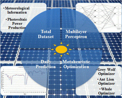
Different from the studies in the literature, the main contribution of this study is to develop the novel hybrid approaches by integrating grey wolf, ant lion and whale optimization algorithms with multilayer perceptron models, and to implement them for the first time in the daily photovoltaic power prediction. Another important contribution is to employ the air temperature, relative humidity, total horizontal solar radiation and diffuse horizontal solar radiation parameters in 4-, 3- and 2-tupled meteorological input structure. The effects of hybrid approaches and multi-tupled meteorological inputs on the prediction performance were revealed in an extensive manner. In addition, all of the prediction results achieved were compared with the persistence reference model for a proper benchmark test. As a result, the hybrid prediction models developed show high success in the daily photovoltaic power prediction.
This paper is organized as follows:
Section 2 explains the hybrid prediction models developed for daily photovoltaic power prediction.
Section 3 introduces the detailed prediction results in terms of different accuracy measures. Finally, conclusions are provided in
Section 4.
2. Hybrid Prediction Models Developed
In this section, multilayer perceptron and grey wolf, ant lion and whale optimization algorithms, which are utilized in the stage of developing the hybrid prediction models, are explained in detail. The architecture of the training sample is shown in
Figure 1. Grey wolf, ant lion and whale optimization algorithms provide the biases and weights of multilayer perceptron, and receive the R
2, MAE and MAPE values for training samples. The variables of multilayer perceptron such as weights and biases are sent to the grey wolf, ant lion and whale optimization algorithms in a series of values for training. Later, the mentioned optimization algorithms recursively change the weights and biases in order to minimize the average error of all training samples. It should be noted that the raw data used in this study were taken from DKA Solar Center in Australia [
22]. It contains a total of 365 one-day measurements covering air temperature, relative humidity, total horizontal solar radiation, diffuse horizontal solar radiation and photovoltaic power production parameters. The units of them are assigned as °C, %, W/m
2, W/m
2 and kW, respectively.
2.1. Multilayer Perceptron
Multilayer perceptron is one of the feed-forward artificial neural networks. Feed-forward artificial neural networks consist of 3 layers, which are called input, hidden and output. Neurons are in the form of regular layers from input to output. There is only a link from one layer to the next layers. The input layer is responsible for transferring the external data to the hidden layer. The hidden layer is responsible for sending the data from input layer to the output layer. In the output layer, the data from hidden layer are processed to produce the output. Therefore, the data coming to the input of the feed-forward artificial neural network are transmitted to the cells in the hidden layer without any change. It is then processed through the output layer and transferred to the external environment, respectively. The structure of multilayer perceptron with a single hidden layer is illustrated in
Figure 2.
The sigmoid, hyperbolic tangent and sinus activation functions used between the layers of multilayer perceptron are given in Equations (1)–(3), respectively [
23]. The sigmoid activation function produces the values between 0 and 1, whereas hyperbolic tangent and sinus activation functions produce the values between −1 and 1. In addition, for the purpose of increasing the consistency of the total dataset, the data are reduced to the range between 0 and 1 by using the min-max normalization method given in Equation (4) [
24].
In addition, we used the persistence reference model, which is also known as Naïve Predictor [
25,
26] and which is widely used for the benchmark tests [
27,
28,
29], in order to compare with other models in this study. In this reference model, the forecasted value at time
t + 1 is equal to the value at time
t. In other words, the persistence reference model is only based on the linear correlation between the present and the future photovoltaic power values. The improvement percentage formula is given in Equation (5), where
is the relevant error of hybrid model and
is the relevant error of persistence method.
2.2. Grey Wolf Optimization Algorithm
The grey wolf optimization algorithm mimics the social hierarchy and hunting behavior of grey wolves [
30]. Grey wolves mostly live in groups and their group size is between 5 and 12 members on average. There are alpha, beta, delta and omega species in which social dominance decreases respectively. The alphas are the most dominant wolves that govern the group best. The betas are the second-level wolves that help the alphas in decision-making or other activities of the group. Omegas are the wolves at the disposal of other wolves that dominate them. If a wolf is not alpha, beta or omega, it is called as the delta. The deltas govern the omegas while serving the alphas and betas. Therefore, the most appropriate solution in the grey wolf optimization algorithm is considered as the alpha (
α). The most appropriate second, third and fourth solutions after the alphas are considered as beta (
β), delta (
δ) and omega (
ω), respectively.
The prey encircling behavior of grey wolves is modeled with Equations (6) and (7).
In these equations, t represents the number of current iterations,
and
represent the coefficient vectors,
represents the position vector of the prey, and
represents the position of a grey wolf.
and
vectors are calculated using Equations (8) and (9). During the iteration, the value of
is reduced linearly from 2 to 0 and
and
are the random vectors in the range [0, 1].
To model the hunting behavior of grey wolves, alpha, beta and delta are taken as the top three best solutions by assuming that they have better knowledge about the potential position of the prey. It is then ensured that other search agents update their positions according to the position of the best search agent. The following equations are used for these operations.
In these equations, is a random value in the range [−2a, 2a]. forces the grey wolves to attack their prey, while forces the grey wolves to move away from the prey to find a more appropriate prey. Finally, the grey wolf optimization algorithm is ended by fulfilling a termination criterion.
2.3. Ant Lion Optimization Algorithm
The ant lion optimization algorithm mimics the interaction between ant lions and ants in their traps [
31]. The life cycle of ant lions consists of two main stages: larvae and adulthood. Natural life cycles of them are up to three years. They spend most of this time as the larvae, and only 3–5 weeks of their life is spent with the adulthood.
Since ants move stochastically when looking for food in nature, a random walk is selected by using Equations (13) and (14).
In these equations,
represents the cumulative sum,
represents the maximum number of iterations,
is the step of random walk,
is a stochastic function and
represents a random number generated with a uniform distribution in the range of [0, 1]. Since each search space has a boundary, Equations (13) and (14) cannot be used directly to update the position of ants. In order to keep the random walk of ants in the search space, normalization is performed at each iteration by using Equation (15).
In this equation represents the minimum of the random walk of the ith variable, represents the maximum of the random walk of the ith variable, represents the minimum of the ith variable at tth iteration and represents the maximum of the ith variable at tth iteration.
The random walks of ants are affected by the traps of ant lions. Equations (16) and (17) are used for modelling this assumption mathematically.
In these equations,
represents the minimum of all variables at tth iteration,
represents the maximum of all variables at tth iteration and
represents the position of
jth ant lion selected at
tth iteration. Ant lions throw sand out of the center of the pit when they realize that an ant is trapped. This behavior causes the trapped ant to slip down. To mathematically model this behavior, the radius of the random walk of ants in a hyper-sphere is adaptively reduced using Equations (18) and (19).
In these equations, , where t represents the current iteration, T represents the maximum number of iterations, and w represents a constant determined according to the current iteration.
When ant reaches the bottom of the pit, and when it is caught in the ant lion’s jaw, the final stage of hunting takes place. After this stage, the ant lion draws the ant into the sand and consumes it. This process is modeled using Equation (20).
In this equation,
indicates the position of
ith ant at
tth iteration. On the other hand, in each iteration, the most suitable ant lion obtained so far is recorded as the elite and it is assumed that all ants walk randomly around a selected ant lion through the roulette wheel in order to be affected by the movement of all ants with the elite. The elite becomes like Equation (21).
In this equation, represents the random walk around the ant lion selected by the roulette wheel at tth iteration, and represents the random walk around the elite at the tth iteration.
2.4. Whale Optimization Algorithm
The whale optimization algorithm mimics the hunting behavior of humpback whales [
32]. In the hunting strategy, which is called as the bubble-net feeding method, humpback whales first dive down to a certain depth. Then, they begin to form bubbles spirally around the prey and swim to the surface. In this way, they both conceal themselves and feed by keeping their prey in the bubble-net. Since the location of the optimal design in the search space is not known in advance, the whale optimization algorithm assumes that the best available candidate solution is target hunting or near optimal. Once the best search agent is identified, other search agents try to update their location according to the best search agent. This behavior is modeled using Equations (6)–(9), similar to the grey wolf optimization algorithm. In addition, during the iteration, the value of
is reduced from 2 to 0, and the shrinking encircling mechanism in the bubble-net feeding method is realized.
On the other hand, Equations (22) and (23) are used for the spiral position update in the bubble-net feeding method. By means of these equations, the spiral motion between the humpback whale position and the prey position is modeled.
In these equations,
represents the distance of
ith whale to the hunt (the best solution so far),
b is a constant for defining the logarithmic spiral shape and
is a random number in the range [−1, 1]. In addition, Equation (24) is used for simultaneously modelling the shrinking encircling mechanism and the spiral position updating of humpback whales around the prey.
In this equation, is a random number in the range [0,1]. As in the grey wolf optimization algorithm, the whales search globally in the case of , while the elite whale is selected and other whales update their positions according to the elite whale in the case of .
3. Daily Photovoltaic Power Prediction
In this section, grey wolf, ant lion and whale optimization algorithms are integrated to the multilayer perceptron algorithm for the daily photovoltaic power prediction. Sigmoid, sinus and hyperbolic tangent activation functions are used in the multilayer perceptron algorithm. The results belong to 2 activation functions, which provide the best prediction performance, are given for each hybrid prediction model developed. In addition, meteorological parameters of air temperature (TA), relative humidity (HR), total horizontal solar radiation (SRTH) and diffuse horizontal solar radiation (SRDH) are used as the multi-tupled input data. The prediction results obtained are compared in terms of the coefficient of determination, mean absolute error and mean absolute percentage error measures.
In the optimization algorithms, which used 4-tupled meteorological input, the number of search agents and the values of lower and upper bounds were assigned as 20, −20 and 20, respectively. In this model, we used nine hidden nodes for the multilayer perceptron algorithm. In the optimization algorithms, which used 3-tupled meteorological inputs, the number of search agents and the values of lower and upper bounds were defined as 20, −10 and 10, respectively. In this model, we used seven hidden nodes for the multilayer perceptron algorithm. In the optimization algorithms, which used 2-tupled meteorological inputs, the number of search agents and the values of lower and upper bounds were assigned as 20, −15 and 15, respectively. In this model, we used five hidden nodes for the multilayer perceptron algorithm. The maximum number of iterations in all optimization algorithms was defined as 250. These characteristic assignments/definitions were determined as a result of the experimental studies. In addition, each hybrid prediction algorithm was run 10 times independently in order to eliminate the unexpected (stochastic) cases. All experiments are executed on a 2.2 GHz Intel (R) Core (TM) personal computer with 8 GB RAM under MATLAB 2016a.
Moreover, the performance of the hybrid prediction models developed was compared with the persistence reference model. The performance of the persistence reference model in the daily photovoltaic power prediction was found as 0.1589 for the coefficient of determination (R2), 0.081 for the mean absolute error (MAE) and 15.702% for the mean absolute percent error (MAPE). In the next subsections, the smallest error results for each input tuple are highlighted in boldface in each table.
3.1. Daily Photovoltaic Power Prediction Using Grey Wolf Optimization Algorithm-Based Multilayer Perceptron (GWO-MLP)
The daily photovoltaic power prediction results for the grey wolf optimization algorithm-based multilayer perceptron, which used the sigmoid activation function, are presented in
Table 1. In case of examining the error values in this table, R
2 of 0.9791, MAE of 0.017 and MAPE of 2.598% were found for air temperature, relative humidity, total horizontal solar radiation and diffuse horizontal solar radiation inputs. Among 3-tupled meteorological inputs, the best prediction performance was obtained as 0.9841 for R
2, 0.016 for MAE and 2.632% for MAPE using air temperature, total horizontal solar radiation and diffuse horizontal solar radiation inputs. Among 2-tupled meteorological inputs, the best prediction performance was obtained as 0.9633 for R
2, 0.022 for MAE and 3.076% for MAPE using total horizontal solar radiation and diffuse horizontal solar radiation inputs.
As a result, among the error results occurred using the sigmoid activation function, the best prediction performance was achieved by the GWO-MLP method, which used air temperature, relative humidity, total horizontal solar radiation and diffuse horizontal solar radiation inputs. The predicted photovoltaic power values that belong to this hybrid method are illustrated in
Figure 3. On the other hand, the worst prediction performance is caused by the GWO-MLP method, which used relative humidity and diffuse horizontal solar radiation inputs, with R
2 of 0.4046, MAE of 0.091 and MAPE of 14.936%.
The daily photovoltaic power prediction results for the grey wolf optimization algorithm-based multilayer perceptron, which used the hyperbolic tangent activation function, are listed in
Table 2. In case of investigating the error values in this table, R
2 of 0.4423, MAE of 0.066 and MAPE of 11.614% were found for air temperature, relative humidity, total horizontal solar radiation and diffuse horizontal solar radiation inputs. Among 3-tupled meteorological inputs, the most accurate prediction performance was obtained as 0.9003 for R
2, 0.032 for MAE and 5.208% for MAPE using air temperature, relative humidity and total horizontal solar radiation inputs. Among 2-tupled meteorological inputs, the most accurate prediction performance was obtained as 0.9508 for R
2, 0.027 for MAE and 4.248% for MAPE using air temperature and total horizontal solar radiation inputs.
In consequence, among the error results occurred using the hyperbolic tangent activation function, the most accurate prediction performance was accomplished by the GWO-MLP method, which used air temperature and total horizontal solar radiation inputs. The predicted photovoltaic power values of this hybrid method are depicted in
Figure 4. However, the most erroneous prediction performance was produced by the GWO-MLP method, which used relative humidity and diffuse horizontal solar radiation inputs, with R
2 of 0.0714, MAE of 0.151 and MAPE of 22.291%.
In case of evaluating the prediction results in general, the GWO-MLP method, which used the sigmoid activation function, shows better prediction performance than the one using the hyperbolic tangent activation function. Furthermore, it respectively improves the R
2, MAE and MAPE in the ratios of 80.62%, 79.01% and 83.45% in comparison to the persistence reference model. Finally, the lowest MAPE values achieved by the GWO-MLP method are visualized in
Figure 5.
3.2. Daily Photovoltaic Power Prediction Using Ant Lion Optimization Algorithm-Based Multilayer Perceptron (ALO-MLP)
The daily photovoltaic power prediction results for the ant lion optimization algorithm-based multilayer perceptron, which used the sigmoid activation function, are presented in
Table 3. In case of examining the error values in this table, R
2 of 0.7101, MAE of 0.068 and MAPE of 12.106% were found for air temperature, relative humidity, total horizontal solar radiation and diffuse horizontal solar radiation inputs. Among 3-tupled meteorological inputs, the best prediction performance was obtained as 0.9334 for R
2, 0.029 for MAE and 4.702% for MAPE using relative humidity, total horizontal solar radiation and diffuse horizontal solar radiation inputs. Among 2-tupled meteorological inputs, the best prediction performance was obtained as 0.9600 for R
2, 0.037 for MAE and 5.959% for MAPE using total horizontal solar radiation and diffuse horizontal solar radiation inputs.
As a result, among the error results occurred using the sigmoid activation function, the best prediction performance was achieved by the ALO-MLP method, which used relative humidity, total horizontal solar radiation and diffuse horizontal solar radiation inputs. The predicted photovoltaic power values of this hybrid method are illustrated in
Figure 6. On the other hand, the worst prediction performance was caused by the ALO-MLP method, which used relative humidity and diffuse horizontal solar radiation inputs, with R
2 of 0.2274, MAE of 0.117 and MAPE of 17.785%.
The daily photovoltaic power prediction results for the ant lion optimization algorithm-based multilayer perceptron, which used the hyperbolic tangent activation function, are listed in
Table 4. In case of investigating the error values in this table, R
2 of 0.3179, MAE of 0.129 and MAPE of 18.232% were found for air temperature, relative humidity, total horizontal solar radiation and diffuse horizontal solar radiation inputs. Among 3-tupled meteorological inputs, the most accurate prediction performance was obtained as 0.8113 for R
2, 0.048 for MAE and 6.738% for MAPE using air temperature, total horizontal solar radiation and diffuse horizontal solar radiation inputs. Among 2-tupled meteorological inputs, the most accurate prediction performance was obtained as 0.8139 for R
2, 0.071 for MAE and 10.430% for MAPE using relative humidity and total horizontal solar radiation inputs.
In consequence, among the error results occurred using the hyperbolic tangent activation function, the most accurate prediction performance was accomplished by the ALO-MLP method, which used air temperature, total horizontal solar radiation and diffuse horizontal solar radiation inputs. The predicted photovoltaic power values of this hybrid method are depicted in
Figure 7. However, the most erroneous prediction performance was produced by the ALO-MLP method, which used relative humidity and diffuse horizontal solar radiation inputs, with R
2 of 0.0117, MAE of 0.137 and MAPE of 21.296%.
In case of evaluating the prediction results in general, the ALO-MLP method, which used the sigmoid activation function, showed better prediction performance than the one, which used the hyperbolic tangent activation function. Besides, it respectively improved the R
2, MAE and MAPE in the ratios of 79.48%, 64.19% and 70.05% in comparison to the persistence reference model. Finally, the lowest MAPE values achieved by the ALO-MLP method are visualized in
Figure 8.
3.3. Daily Photovoltaic Power Prediction Using Whale Optimization Algorithm-Based Multilayer Perceptron (WOA-MLP)
The daily photovoltaic power prediction results for the whale optimization algorithm-based multilayer perceptron, which used the sigmoid activation function, are presented in
Table 5. In case of examining the error values in this table, R
2 of 0.8362, MAE of 0.050 and MAPE of 7.316% were found for air temperature, relative humidity, total horizontal solar radiation and diffuse horizontal solar radiation inputs. Among 3-tupled meteorological inputs, the best prediction performance was obtained as 0.8985 for R
2, 0.040 for MAE and 6.187% for MAPE using air temperature, relative humidity and total horizontal solar radiation inputs. Among 2-tupled meteorological inputs, the best prediction performance was obtained as 0.8959 for R
2, 0.034 for MAE and 5.514% for MAPE using total horizontal solar radiation and diffuse horizontal solar radiation inputs.
As a result, among the error results occurred when using the sigmoid activation function, the best prediction performance was achieved by the WOA-MLP method, which used total horizontal solar radiation and diffuse horizontal solar radiation inputs. The predicted photovoltaic power values of this hybrid method are illustrated in
Figure 9. On the other hand, the worst prediction performance was caused by the WOA-MLP method, which used relative humidity and diffuse horizontal solar radiation inputs, with R
2 of 0.0085, MAE of 0.156 and MAPE of 24.905%.
The daily photovoltaic power prediction results for the whale optimization algorithm-based multilayer perceptron, which used the sinus activation function, are listed in
Table 6. In case of investigating the error values in this table, R
2 of 0.4817, MAE of 0.086 and MAPE of 13.394% were found for air temperature, relative humidity, total horizontal solar radiation and diffuse horizontal solar radiation inputs. Among 3-tupled meteorological inputs, the most accurate prediction performance was obtained as 0.8242 for R
2, 0.045 for MAE and 7.028% for MAPE using air temperature, total horizontal solar radiation and diffuse horizontal solar radiation inputs. Among 2-tupled meteorological inputs, the most accurate prediction performance was obtained as 0.7009 for R
2, 0.075 for MAE and 11.892% for MAPE using total horizontal solar radiation and diffuse horizontal solar radiation inputs.
In consequence, among the error results occurred when using the sinus activation function, the most accurate prediction performance was accomplished by the WOA-MLP method, which used air temperature, total horizontal solar radiation and diffuse horizontal solar radiation inputs. The predicted photovoltaic power values of this hybrid method are depicted in
Figure 10. However, the most erroneous prediction performance was produced by the WOA-MLP method, which used air temperature and total horizontal solar radiation inputs, with R
2 of 0.2667, MAE of 0.186 and MAPE of 25.967%.
In case of evaluating the prediction results in general, the WOA-MLP method, which used the sigmoid activation function, showed better prediction performance than the one which used the sinus activation function. Besides, it improved the R
2, MAE and MAPE in the ratios of 78.43%, 58.02% and 64.88%, respectively in comparison to the persistence reference model. Finally, the lowest MAPE values achieved by the WOA-MLP method are visualized in
Figure 11.
In a nutshell, the observed photovoltaic power values and the predicted photovoltaic power values of GWO-MLP, ALO-MLP, WOA-MLP hybrid models and persistence reference model are illustrated in
Figure 12.


