Article

Linear-Gompertz Model-Based Regression of Photovoltaic Power Generation by Satellite Imagery-Based Solar Irradiance

1
New-Renewable Energy Resource & Policy Center, Korea Institute of Energy Research, Daejeon 34129, Korea
2
Higher Polytechnic School, University of Lleida, 25001 Lleida, Spain
*
Author to whom correspondence should be addressed.
Energies 2020, 13(4), 781; https://doi.org/10.3390/en13040781
Submission received: 31 December 2019 / Revised: 4 February 2020 / Accepted: 8 February 2020 / Published: 11 February 2020

Abstract

:
A simple yet accurate photovoltaic (PV) performance curve as a function of satellite-based solar irradiation is necessary to develop a PV power forecasting model that can cover all of South Korea, where more than 35,000 PV power plants are currently in operation. In order to express the nonlinear power output of the PV module with respect to the hourly global horizontal irradiance derived from satellite images, this study employed the Gompertz model, which is composed of three parameters and the sigmoid equation. The nonphysical behavior of the Gompertz model within the low solar irradiation range was corrected by combining a linear equation with the same gradient at the conjoint point. The overall fitness of Linear-Gompertz regression to the 242 PV power plants representing the country was R2 = 0.85 and nRMSE = 0.09. The Gompertz model coefficients showed normal distributions and equivariance of standard deviations of less than 15% by year and by season. Therefore, it can be conjectured that the Linear-Gompertz model represents the whole country’s PV system performance curve. In addition, the Gompertz coefficient C, which controls the growth rate of the curve, showed a strong correlation with the capacity factor, such that the regression equation for the capacity factor could be derived as a function of the three Gompertz model coefficients with a fitness of R2 = 0.88.

1. Introduction

Global warming is projected to increase by 1.5 °C between 2030 and 2052. Therefore, public health, human security, and economic growth are expected to face a major threat at the global level in the relatively near future [1]. In South Korea, greenhouse gas emissions from the energy sector, which accounted for 87% of total emissions in 2014, declined by 1.2% compared with the previous year due to the implementation of an energy transition strategy in which fossil fuel power plants are being replaced by renewable energy [2,3].
The implementation of the energy transition plan “Renewable Energy 3020”, which was announced in 2017, will increase the renewable energy share of the energy mix from its current level of 7% to 20% by 2030, thus providing a new power capacity of 48.7 GW. “Renewable Energy 3020” has become the foremost driver toward the installation of photovoltaic (PV) systems [4]. As a result, South Korea has been ranked among the top 10 PV markets in terms of cumulative capacity, having reached 7.2 GW in 2018, and there are plans to install further 30.8 GW by 2030 [5].
Once renewable power generation accounts for over 20% of electricity generation, the stability of the electricity grid will be an important issue due to the volatility of solar and wind energy. In order to resolve this problem, renewable energy forecasting has been proposed as a major solution for stable management of the electricity [6]. Especially for long-term forecasting, first, solar irradiation should be predicted based on either numerical weather prediction or satellite imagery, and second, PV power output should be estimated by a performance curve of a PV system using solar irradiance as the input [7].
Recently, the prediction of solar irradiance from satellite imagery using radiative transfer models was adopted [8]. The University of Arizona Solar Irradiance Based on Satellite/Korea Institute of Energy Research (UASIBS-KIER) model of Kim et al. [9] reliably produces down-welling surface shortwave radiation every 15 min at a 1-km2 spatial resolution by employing the geostationary weather satellite COMS (Communication, Ocean, and Meteorological Satellite), which was launched in 2010 and scans the Oceanian hemisphere.
Not only PV power forecasting for peak load control, but also evaluations of PV potential for the establishment and management of the national supply target, require a simple yet reliable performance curve of PV systems as a function of solar irradiance [10]. Therefore, the primary purpose of this study was to derive a generalized performance curve of PV systems by correlating the PV power output of the nation’s PV power plants and the satellite imagery-based solar irradiance at their locations all over the country.
Sharma et al. (2010) [11] and Zhanga et al. (2018) [12] applied the linear regression of solar irradiance and PV power output to develop a PV power forecasting model, which was also the purpose of the present study. Gan et al. (2015) [13] and Field et al. (2015) [14] fitted PV power and solar irradiance with the fourth- and fifth-order polynomial equations, respectively, which was problematic because a high-order polynomial equation exhibits an unexpected curved shape outside the fitting value range.
This paper introduced the Gompertz model, a sigmoidal equation commonly used in growth analyses, as an adequate regression model for determining the PV performance curve, i.e., PV power output with respect to global horizontal irradiance (GHI). In order to correct an inconsistency of the Gompertz model and the real PV power output in low GHI ranges, a linear equation was conjoined. The regression model parameters were determined using the hourly PV power output data of 232 sites across the country for a three-year period, and the corresponding hourly GHI was predicted using the UASIBS-KIER model.

2. Data

2.1. Solar Irradiance Data

The UASIBS-KIER model estimates the GHI based on the visible reflectance and infrared brightness temperature taken from COMS satellite imagery over the Korean Peninsula. The GHI is usually derived from the look-up table pre-generated by the Goddard Space Flight Center Radiative Transfer Model [15] to obtain discrete values of the solar zenith angle, surface albedo, ozone, water vapor, aerosol/clout optical depths, and so forth. The accuracy of the UASIBS-KIER model was validated to be the root mean square error of 9.1% and 15.5% for clear and cloudy skies, respectively, by comparing it with 35 ground observation stations [16].
The plane-of-array irradiance (POA), rather than the GHI, is the solar irradiance component that contributed directly to the PV module’s performance. In order to evaluate the POA, not only the installation layout of the PV panel—such as the installation angle and direction—but also the direct normal insolation (DNI) should be calculated by the direct-diffuse irradiance decomposition of the GHI. Because the aforementioned work has yet to be completed, the verified GHI data were employed first.

2.2. PV Power Generation Data

In 2018, the number of PV power plants in South Korea was about 35,000 of which we filtered the power generation data of 600 PV power plants (N = 600) which were grid connected, registered with the Korea Power Exchange (KPX), had over 50 kW capacity, and were in operation during the period January 2014 to December 2016.
The sample size (n), determined using the Cochran method [17]; Equations (1) and (2), was 234, which represents 39% of N with a 95% confidence level (z = 1.96) and ±5% precision (e = 0.05).
n = n 0 1 + n 0 1 N
n 0 = z 2 · p · ( 1 p ) e 2
The stratified random sampling method was used to calculate the appropriate size of the sample for each province, which accounted for 242 if the numbers were rounded up, with the study sample being larger than 40% of the total number of PV power plants in the country (Table 1). Almost 50% of the PV power plants were located in Jeollanam-do and Gyeongsangbuk-do (Figure 1).
The 10 randomly selected PV power plants were reserved for the validation test of statistical regression, meaning that the dataset of 10 sites was not used for creating the model.
According to Jordan and Kurtz (2013) [18], the median performance degradation due to the aging of the PV module was estimated to be −0.5%p per year. The mean life of the 242 PV power plants used in this study was 4.6 years so that the estimated overall degradation rate was -2.3% p. However, only three years of PV power output data were used in this study, which was insufficient to enable a statistical analysis of the aging trend. Moreover, it was difficult to identify the aging effect before excluding the other effects caused by various environmental conditions. For these reasons, this study did not consider the aging effect.

3. Methods

3.1. Regression Model

3.1.1. Gompertz Function

Figure 2 shows a typical PV module performance with respect to solar irradiation. Because of the nonlinearity of the PV module performance [19], a linear regression depicted as a dashed line was unsuitable for expressing the performance curve of the PV module.
The Gompertz function is a sigmoid curve, which describes asymptotic growth as being the slowest at the end of a given time period or at the maximum of a given variable. With regard to the solar energy field, a symmetrized and shifted Gompertz function was applied to model the I-V curve of the PV module [20].
Therefore, the performance curve of the PV system as the Gompertz function of GHI (W/m2) was expressed as the following equation:
P P N = A · e e B C · G H I
where A is the asymptote, B is the x-axis displacement, and C is the growth rate.
First, the hourly PV power output P (kW) at each power plant was normalized by dividing it by its nominal capacity PN (kW). Second, a regression analysis was conducted to find the best fitness between the hourly GHI and the normalized PV power output by employing the Gompertz function.
Figure 3 shows the effects of the coefficients: A controlled the asymptote maximum upward and downward, B shifted the curve left and right, and C changed the growth rate. Its sigmoid shape was asymmetrical and had an inflection point that converges to a maximum value, which was ideally PN, as the PV power output generally bended to the nominal capacity.

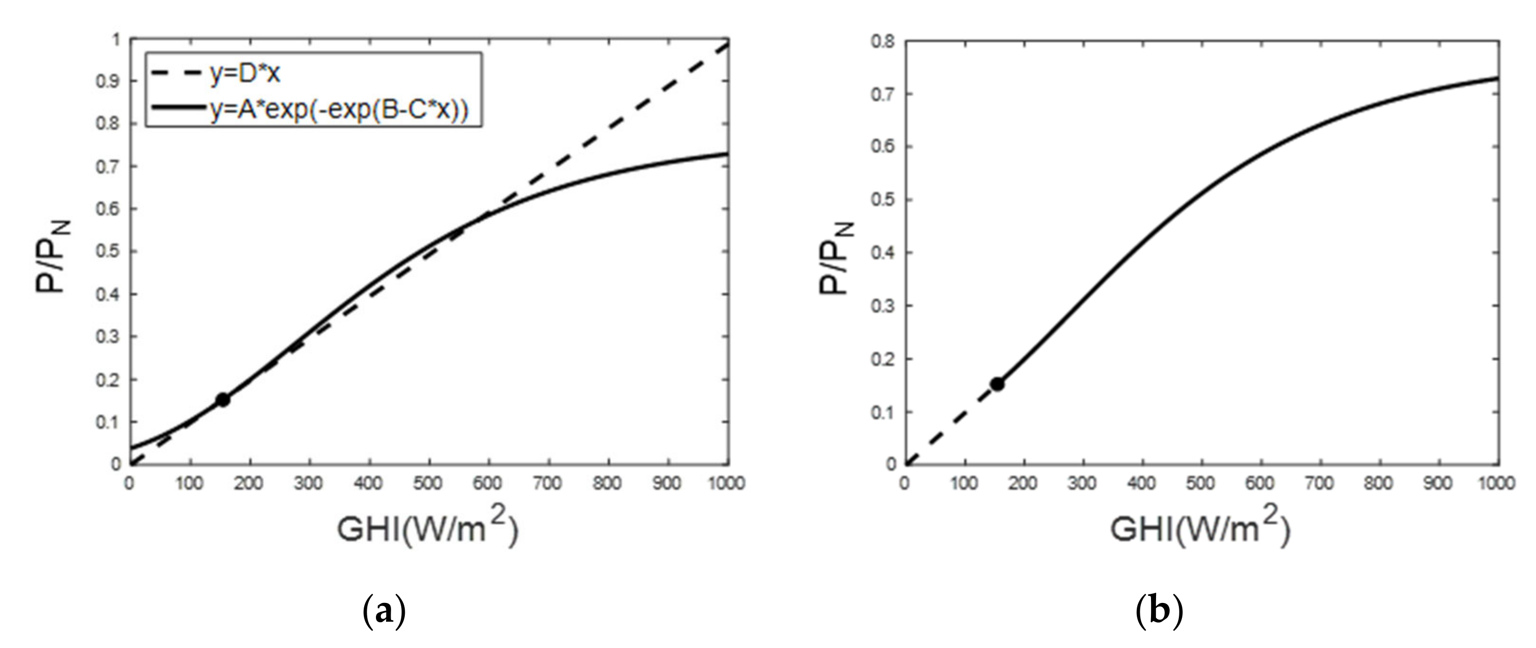
3.1.2. Linear-Gompertz Conjoint Function

The Gompertz curve poorly represents the correlation between GHI and P near the origin, which means that y converges to A · e e B as x approaches zero. This mathematical behavior violates the laws of physics, i.e., the PV power output should be zero when there is no solar irradiance.
In order to prevent this nonrealistic behavior of the regression model, a linear equation having the slope D with a y-intercept of zero was combined to the Gompertz function near the origin [21].
The conjoint curve was expressed as follows:
y = { D ( x x j ) A · e e B C · x ( x > x j )
For a smooth connection of the two curves, it was necessary to impose the following conjoint conditions:
y | x = x j = D · x j = A · e e B C · x j
d y d x | x = x j = D = A · C · e e B C · x j · e B C x j
where ( x j , y j ) is the connection point of the two functions.
By substituting Equation (6) with Equation (5), the following equation was obtained:
C · x j · e B C · x j = 1
Equation (7) can be solved analytically by introducing the Lambert W-function [22], and the following solution was obtained:
x j = W ( e B ) C
where W(z) is the Lambert W-Function, the inverse function of f ( v ) = v · e v . There were multiple solutions for xj, but the smallest xj was chosen for the present study.
Figure 4 demonstrates the conjoint case when (A, B, C) = (0.77, 1.10, 0.004). Once the Gompertz coefficients were derived by regression analysis, it was possible to calculate xj by Equation (8), D by Equation (6), and finally, yj by Equation (4).

3.2. Evaluation of Regression

The fitness of the regression model was evaluated with the normalized root mean square error (nRMSE) with respect to the nominal capacity PN, which was defined as:
n R M S E = 1 T · i = 1 T ( P L G , i P K P X , i ) 2 / P N
where T is the total number of power generation hours (P > 0), and PL-G and PKPX stand for the PV power predicted by the Linear-Gompertz (L-G) regression model and the real PV power output data provided by KPX, respectively.
The coefficient of determination (R2) was also evaluated for the linear regression (as the reference) and the Linear-Gompertz regression for comparison. The evaluation of regression was carried out by year, by season, and by province to confirm whether the Linear-Gompertz model was suitable as the PV performance curve. The final validation was performed for the 10 sites, which were not used to derive the Gompertz model coefficients.

4. Results and Discussions

4.1. Comparison of the Regression Models

Regression fitness, as measures of R2 and nRMSE, was evaluated for the 232 PV power plants, excluding the 10 sites which were reserved for validation. Table 2 compares the mean (μ) and the standard deviation (σ) of the fitness measures between the Linear (L) model and the Linear-Gompertz model by year. Of the overall values of the measures, the fitness of L-G was better than L, as R2 was higher and nRMSE was lower for the L-G regression. For the statistical confirmation, t-tests assuming equal means (Equation (10)) were performed, resulting in the rejection of the null hypothesis (p-values < 0.05), which confirms that the means of L and L-G were statistically different. In other words, R2 and nRMSE of L-G were statistically higher than those of L by about 2.5% and 11% respectively.
It was difficult to determine whether the L-G model substantially outperformed the L model because the solar irradiance in South Korea was not strong (<1300 W/m2) and most of the GHI and PV power output data were concentrated in the linear section (<1000 W/m2) of the L-G regression model. However, the comparison results obtained after selecting 10 PV power plants of high solar irradiance in excess of 1000 W/m2 verified that the R2 improvement in the L-G model was 6%, which is significantly higher than 2.6%.
μ L G μ L = 0
Figure 5 shows the spatial distribution of R2 and nRMSE of the Gompertz model over South Korea, in which no obvious spatial pattern can be observed, i.e., a random pattern was present. For reference, the correlation coefficient between R2 and nRMSE was −0.86.

4.2. Gompertz Model Coefficients

Before proceeding with the statistical analysis, the Anderson–Darling [23] normality tests for A, B, and C, which constitute an effective normality test for small samples, were carried out. The results of the normality test confirmed that all of the Gompertz coefficients had a normal distribution.
The means and standard deviations of the Gompertz coefficients derived from the regression of 232 sites are summarized in Table 3. As Table 3 shows, the means of A and B varied slightly from year to year, but the standard deviations of all the coefficients did not vary according to the equal variance F-test. Moreover, the standard deviations of A and B varied within 6.5% of their means, while C showed a wider variation of 15%. Given that the statistical characteristics of the Gompertz coefficients had normal distributions, equivariance, and small standard deviations, it is possible to conclude that the Gompertz coefficients represent the whole country’s PV system performance characteristics.
Figure 6 shows comparison of the Gompertz curves by province. The standard deviations of these curves obtained from the generalized Gompertz curve, whose coefficients are given in Table 3, were within 5% across the whole GHI range.
Figure 7 shows the relationship between the Gompertz coefficient C and the capacity factor (CF) of the 232 sites. It can clearly be seen that the capacity factor and the Gompertz coefficient C had a strong correlation of R2 = 0.53, while the Gompertz coefficients A and B showed no correlation with the capacity factor (R2 < 0.02). This can be interpreted to mean that the Gompertz coefficient C controlled the variance of the curve at a given solar irradiance depending on such environmental factors as air temperature. Therefore, it was necessary to analyze the Gompertz coefficient by season in order to identify the effects of air temperature.
Using the strong correlation between C and CF, it was possible to derive an equation for CF as a function of the Gompertz coefficients through a multivariate regression, as follows:
C F = 17.3 · A 6.7 · B + 2579.6 · C 1.9
For reference, the regression fitness of Equation (11) showed a fitness of R2 = 0.88, which was higher than that of C and CF, by accommodating the interconnected relationship between C and A, as well as B.
The variations of the Gompertz coefficient by season (as listed in Table 4) were evaluated in order to ascertain whether the ambient temperature had a major impact on the plants’ performance. It is well-known that the PV module’s efficiency decreases when its temperature rises to a certain threshold value, adversely affecting summertime power production [24].
Figure 8 illustrates this phenomenon with a comparison of PV power output between winter and summer.
The seasonal variations of the Gompertz coefficients A, B, and C with respect to their annual means were 16%, 20%, and 32%, respectively (Table 4). This implies that the Gompertz coefficient C (or capacity factor) had obvious seasonality due to changes of the environmental parameters by season, such as the ambient temperature. In terms of the capacity factor, winter, autumn, spring, and summer were from the highest to lowest order. The fitness of the seasonal Gompertz model increased to R2 = 0.88.

4.3. Validation of the Model

Table 5 summarizes the results of the validation of the generalized Linear-Gompertz model given in Equation (4) with the mean values given in Table 3. It is confirmed that the fitness measures showed the same level of R2 and nRMSE, as shown in Table 2.
These conclusions mean that if the PV power generation was estimated using the L-G model throughout South Korea, the expected nRMSE was 0.09, which is 10% of the PN. This error includes not only the error of the regression model, but also that of the input data GHI. According to a study conducted by Kim et al. (2017), the GHI prediction of the UASIBS-KIER model ranged between 7.4%~16.7% in terms of the rRMSE [16]. This level of error is sufficient for the purpose of evaluating the PV potential of South Korea. However, considering that the average rate of error of general one-hour-ahead forecasting models is nRMSE = 7.2% [25], the error in the results of the present study is somewhat large for a PV power forecasting model.

5. Conclusions

The following conclusions may be drawn based on the statistical analysis of the hourly correlation between the power output of 242 PV power plants (out of a total of 35,000 power plants) in South Korea in 2018, and the weather satellite-derived solar irradiation on their installation locations.
The main results of this study are summarized as follows:
(1)
The Linear-Gompertz model successfully expressed the sigmoidal characteristics of the PV system performance countrywide as a single function of GHI, which is the simplest regression form adequate for machine learning needed to develop a forecasting model. The nonphysical trend of the Gompertz model in the low GHI range was fixed by combining a linear equation having the same slope at the conjoint point. The fitness of the Linear-Gompertz regression was R2 = 0.85, and the nRMSE of normalized power output ratio was 0.09.
(2)
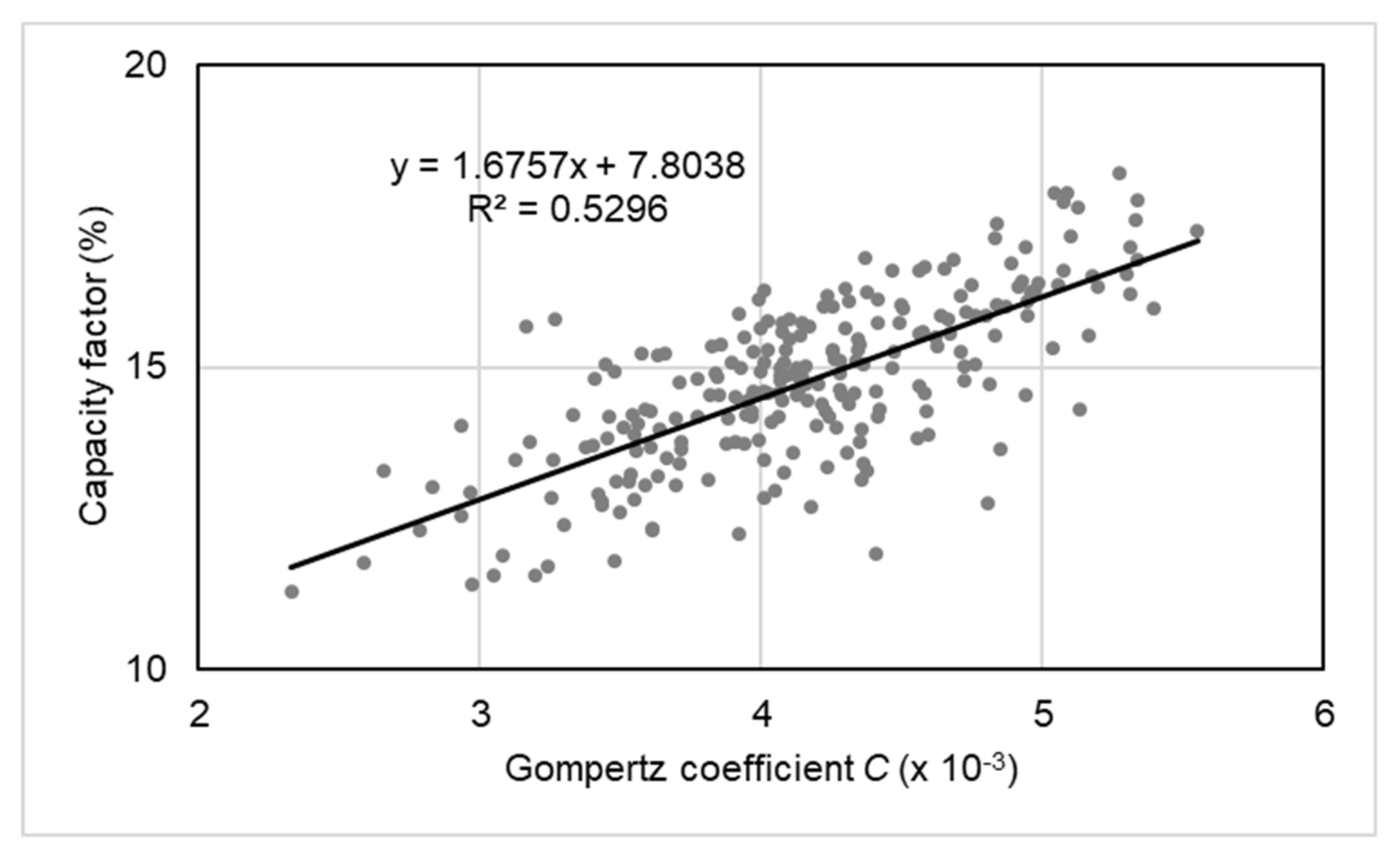
The three Gompertz coefficients A, B, and C were calculated by year, by season, and by province, and it was found that they had normal distributions and equivariances, meaning that the Gompertz coefficients were the general parameters for the entire country. Moreover, the Gompertz coefficient of the growth rate C showed a strong correlation (R2 = 0.53) with the capacity factor of the PV power plant. Therefore, it was possible to derive the capacity factor equation as a function of A, B, and C, that showed a fitness of R2 = 0.88.
(3)
In order to use the Linear-Gompertz model to obtain South Korea’s general PV performance curve for PV power forecasting, it will be necessary to increase the fitness of the model to over R2 > 0.9 by including significant environmental variables such as ambient temperature. Future research will consist of securing long-term PV power output data and analyzing the aging effect of the PV panel to correct the degradation effect. In addition, the accuracy of the Linear-Gompertz model will be improved by calculating and applying the POA, the primary input variable, instead of GHI. To that end, the solar irradiance decomposition algorithm should be improved in the UASIBS-KIER model, and verification and compensation steps using actual measurement data should be implemented in advance.
(4)
Because the solar irradiance in most regions of South Korea is less than 1300 W/m2, an additional verification of the conditions of high solar irradiance is needed to apply this result to regions with high solar irradiance. In addition, since PV power generation is significantly influenced by climate conditions, there will be some differences compared to regions in which the climate zone is completely different from that of South Korea. However, South Korea has four distinct seasons and a wide temperature distribution ranging from −15 °C to +35 °C throughout the year. Thus, the effect of climate conditions on PV power generation is relatively significant, which means the prediction error that occurred when the present regression model was applied to other climate zone is expected to be smaller in a relative sense.

Author Contributions

H.-G.K. designed and supervised the research; A.V. and B.-Y.K. conceived a novel idea; C.K.K. contributed to data curation; A.V. and H.-G.K. wrote the paper. All authors have read and agreed to the published version of the manuscript.

Funding

This work was conducted under the framework of the Research and Development Program of the Korea Institute of Energy Research (C0-2407).

Conflicts of Interest

The authors declare no conflict of interest.

References

  1. IPCC. Summary for Policymakers. In Global warming of 1.5°C. An IPCC Special Report on the impacts of global warming of 1.5°C above pre-industrial levels and related global greenhouse gas emission pathways, in the context of strengthening the global response to the threat of climate change, sustainable development, and efforts to eradicate poverty, 1st ed.; World Meteorological Organization: Geneva, Switzerland, 2018. [Google Scholar]
  2. Greenhouse Gas Inventory and Research Center. Second Biennial Update Report of the Republic of Korea Under the United Nations Framework Convention on Climate Change, 1st ed.; The Government of the Republic of Korea: Seoul, Korea, 2017; pp. 25–33.
  3. Maennel, A.; Kim, H.-G. Comparison of greenhouse gas reduction potential through renewable energy transition in South Korea and Germany. Energies 2018, 11, 206. [Google Scholar] [CrossRef] [Green Version]
  4. Korea Energy Agency. 2018 New & Renewable Energy White Paper, 1st ed.; Korea Ministry of Trade, Industry and Energy: Seoul, Korea, 2019.
  5. SolarPower Europe. Global Market Outlook for Solar Power/2018–2022, 1st ed.; SolarPower Europe: Brussels, Belgium, 2018; p. 64. [Google Scholar]
  6. Wirth, H. Recent Facts about Photovoltaics in Germany, 1st ed.; Fraunhofer Institute for Solar Energy Systems: Freiburg, Germany, 2019. [Google Scholar]
  7. Das, U.K.; Tey, K.S.; Seyedmahmoudian, M.; Mekhilef, S.; Idris, M.Y.I.; van Deventer, W.; Horan, B.; Stojcevski, A. Forecasting of photovoltaic power generation and model optimization: A review. Renew. Sustain. Energy Rev. 2018, 81, 912–928. [Google Scholar] [CrossRef]
  8. Ruiz-Ariasa, J.A.; Gueymard, C.A. Worldwide inter-comparison of clear-sky solar radiation models: Consensus based review of direct and global irradiance components simulated at the earth surface. Solar Energy 2018, 168, 10–29. [Google Scholar] [CrossRef]
  9. Kim, C.K.; Holmgren, W.F.; Stovern, M.; Betterton, E.A. Toward improved solar irradiance forecasts: Derivation of downwelling surface shortwave radiation in Arizona from satellite. Pure Appl. Geophys. 2016, 173, 2535–2553. [Google Scholar] [CrossRef]
  10. Bocca, A.; Bergamasco, L.; Fasano, M.; Bottaccioli, L.; Chiavazzo, E.; Macii, A.; Asinari, P. Multiple-Regression Method for Fast Estimation of Solar Irradiation and Photovoltaic Energy Potentials over Europe and Africa. Energies 2018, 11, 3477. [Google Scholar] [CrossRef] [Green Version]
  11. Sharma, N.; Gummeson, J.; Irwin, D.; Shenoy, P. Cloudy computing: Leveraging weather forecasts in energy harvesting sensor systems. In Proceedings of the 7th Annual IEEE Communications Society Conference on Sensor, Mesh and Ad Hoc Communications and Networks (SECON), Boston, MA, USA, 21–25 June 2010; pp. 1–9. [Google Scholar]
  12. Zhanga, W.; Danga, H.; Simoes, R. A new solar power output prediction model based on a hybrid forecast engine and a decomposition model. ISA Trans. 2018, 81, 105–120. [Google Scholar] [CrossRef] [PubMed]
  13. Gan, L.K.; Shek, J.K.H.; Mueller, M.A. Hybrid wind–photovoltaic–diesel–battery system sizing tool development using empirical approach, life-cycle cost and performance analysis: A case study in Scotland. Energy Conv. Manag. 2015, 106, 479–494. [Google Scholar] [CrossRef] [Green Version]
  14. Field, D.A.; Rogers, T.; Sealy, A. Dust accumulation and PV power output in the tropical environment of Barbados. In Proceedings of the 14th International Conference on Sustainable Energy Technologies, Nottingham, UK, 25–27 August 2015; pp. 276–278. [Google Scholar]
  15. Chou, M.-D.; Suárez, M.J. A solar radiation parameterization for atmospheric studies. NASA Tech. Rep. Series Global Model. Data Assim. 1999, 15, 1–40. [Google Scholar]
  16. Kim, C.K.; Kim, H.-G.; Kang, Y.-H.; Yun, C.-Y. Toward improved solar irradiance forecasts: Comparison of the global horizontal irradiances derived from the COMS satellite imagery over the Korean Peninsula. Pure Appl. Geophys. 2017, 174, 2773–2792. [Google Scholar] [CrossRef]
  17. Cochran, W.G. Sampling Techniques, 3rd ed.; John Wiley & Sons, Inc.: New York, NY, USA, 1977; pp. 72–88. [Google Scholar]
  18. Jordan, D.C.; Kurtz, S.R. Photovoltaic degradation rates—An analytical review. Prog. Photovol. Res. Appl. 2013, 21, 12–29. [Google Scholar] [CrossRef] [Green Version]
  19. King, D.L.; Boyson, W.E.; Kratochvil, J.A. Photovoltaic Array Performance Model, SAND2004-3535; Sandia National Laboratories: Albuquerque, NM, USA, 2004. [Google Scholar]
  20. Molina-Garcia, A.; Guerrero-Pérez, J.; Bueso, M.C.; Kessler, M.; Gómez-Lázaro, E. A new solar module modeling for PV applications based on a symmetrized and shifted Gompertz model. IEEE Trans. Energy Conv. 2015, 30, 51–59. [Google Scholar] [CrossRef]
  21. Kim, B.Y.; Vilanova, A.; Kim, C.K.; Kang, Y.H.; Yun, C.Y.; Kim, H.G. Non-linear regression model between solar irradiation and PV power generation using the Gompertz curve. J. Korean Solar Energy Soc. 2019, 39, 113–125. [Google Scholar] [CrossRef]
  22. Georg, O.; Szegö, G. Aufgaben und Lehrsätze aus der Analysis; Springer-Verlag: Heidelberg, Germany, 2013; Volume 74. [Google Scholar]
  23. Anderson, T.W.; Darling, D.A. A Test of goodness of fit. J. Am. Stat. Assoc. 1954, 49, 765–769. [Google Scholar] [CrossRef]
  24. Shravanth, V.M.; Srinivasan, J.; Ramasesha, S.K. Performance of solar photovoltaic installations: effect of seasonal variations. Solar Energy 2016, 131, 39–46. [Google Scholar] [CrossRef] [Green Version]
  25. Cheon, J.H.; Lee, J.T.; Kim, H.G.; Kang, Y.H.; Yun, C.Y.; Kim, C.K.; Kim, B.Y.; Kim, J.Y.; Park, Y.Y.; Kim, T.H.; et al. Review of the trend of solar energy forecasting techniques. J. Korean Solar Energy Soc. 2019, 39, 41–54. [Google Scholar] [CrossRef]
Figure 1. Provincial distribution of the sample PV power plants (the blue symbols correspond to the 10 validation plants).
Energies 13 00781 g001
Figure 2. The scatterplot between the PV power output and the global horizontal irradiance (GHI; Jeollanam-do, Youngkwang-gun, 300 kW).
Energies 13 00781 g002
Figure 3. Effects of the Gompertz model coefficient: (a) effect of A (B = 1.10, C = 4·10−3), (b) effect of B (A = 0.77, C = 4·10−3), and (c) effect of C (A = 0.77, B = 1.10).
Energies 13 00781 g003
Figure 4. Conjoint process of a linear line (dashed line) and a Gompertz curve (solid line). The line and Gompertz curve appear separated in (a) and conjoined in (b).
Energies 13 00781 g004
Figure 5. Distribution of the Gompertz model fitness measures: (a) coefficient of determination (R2) distribution, and (b) normalized root mean square error (nRMSE) distribution.
Energies 13 00781 g005
Figure 6. Comparison of the Gompertz curves by province (for 2014~2016).
Energies 13 00781 g006
Figure 7. The relationship between the Gompertz coefficient C and the capacity factor (mean capacity factor = 14.8 ± 1.4%).
Energies 13 00781 g007
Figure 8. Comparison of the PV system performance curves between summer and winter (Jeollabuk-do Gochang-gun, 500 kW).
Energies 13 00781 g008
Table 1. Provincial distribution of the sample photovoltaic (PV) power plants.
ProvinceSamplingPV Plants (>50 kWp)Total No. of PV Plants
Jeollanam-do862186728
Jeollabuk-do28719040
Gyeongsangnam-do29722398
Gyeongsangbuk-do37913847
Chungcheongnam-do16394323
Chungcheongbuk-do6132144
Gyeonggi-do17393435
Gangwon-do9232320
Jeju-do1434590
Sum24260034,825
Table 2. Regression fitness of the Linear and Linear-Gompertz models by year.
Year2014201520162014~2016
ModelLL-GLL-GLL-GLL-G
R20.830.850.840.860.820.850.830.85
nRMSE0.100.090.100.090.100.090.100.09
Table 3. The means and standard deviations of the Gompertz coefficients by year.
Year2014201520162014~2016
Aμ0.770.780.760.77
σ0.050.050.050.05
Bμ1.091.101.101.10
σ0.060.060.060.06
Cμ (×10−3)4.204.094.154.14
σ (×10−3)0.640.620.600.61
Table 4. Seasonal variations of the Gompertz model coefficients by year.
CoefficientSeason2014201520162014~2016
AWinter0.820.870.830.84
Spring0.870.860.860.86
Summer0.740.780.790.77
Autumn0.700.750.730.73
BWinter1.161.171.151.16
Spring1.061.071.091.07
Summer0.960.930.960.95
Autumn0.841.001.110.98
C (×10−3)Winter4.854.624.714.73
Spring3.573.633.553.59
Summer3.723.333.273.44
Autumn4.574.214.504.43
Table 5. Results of validation of the generalized Gompertz model by year.
Year2014201520162014~2016
CodeR2nRMSER2nRMSER2nRMSER2nRMSE
17300.830.100.850.090.840.090.840.09
18370.870.090.890.090.870.090.880.09
18820.880.080.890.080.870.080.880.08
19470.870.090.880.090.870.090.870.09
19960.810.100.820.100.820.100.820.10
88770.860.100.860.100.840.100.850.10
89070.850.090.890.090.860.090.870.09
95770.880.100.880.090.870.090.880.09
96170.890.080.890.080.900.080.890.08
99270.890.090.890.090.890.090.890.09
Mean0.860.090.870.090.860.090.870.09

