Article

Energy Footprint of Mechanized Agricultural Operations

by
Maria Lampridi
1,2,*,
Dimitrios Kateris
1,
Claus Grøn Sørensen
3 and
Dionysis Bochtis
1
1
Center for Research and Technology Hellas (CERTH), Institute for Bio-Economy and Agri-technology (IBO), 6th km Charilaou-Thermi Rd., 57001 Thessaloniki, Greece
2
School of Agriculture, Faculty of Agriculture, Forestry and Natural Environment, Aristotle University of Thessaloniki, 54124 Thessaloniki, Greece
3
Department of Engineering, Aarhus University, Blichers Allé 20, P.O. Box 50, 8830 Tjele, Denmark
*
Author to whom correspondence should be addressed.
Energies 2020, 13(3), 769; https://doi.org/10.3390/en13030769
Submission received: 19 December 2019 / Revised: 4 February 2020 / Accepted: 7 February 2020 / Published: 10 February 2020
(This article belongs to the Special Issue Supply Chain Management for Bioenergy and Bioresources)

Abstract

:
The calculation of the energy cost of a cultivation is a determining factor in the overall assessment of agricultural sustainability. Most studies mainly examine the entire life cycle of the operation, considering reference values and reference databases for the determination of the machinery contribution to the overall energy balance. This study presents a modelling methodology for the precise calculation of the energy cost of performing an agricultural operation. The model incorporates operational management into the calculation, while simultaneously considering the commercially available machinery (implements and tractors). As a case study, the operation of tillage was used considering both primary and secondary tillage (moldboard plow and field cultivator, respectively). The results show the importance of including specific operation parameters and the available machinery as part of determining the accurate total energy consumption, even though the field size and available time do not have a significant effect.

1. Introduction

The concept of agricultural sustainability has been a highly debated subject in recent years, not only because of its importance with respect to evaluating the agri-food system, but mostly because of its multivariate nature [1]. In fact, there is a large number of parameters that are considered with respect to the primary production of agricultural products [2]. These parameters include not only the relevant material flows (e.g., water, fuel, fertilizers, seeds, and crops), but also the means of production, which include labor and the use of agricultural machinery along with the inclusion of operation management [3]. The integration of the individual evaluation of each of those parameters with respect to their contribution to sustainability concerns more and more researchers in recent years. However, agricultural sustainability is approached in a variety of ways in the literature, examining, individually or in combination, economic, environmental, and social indicators [4]. These indicators attempt to assess the impacts of agriculture in a quantitative or a qualitative manner. Several indicators as well as indicator indexes and frameworks have been proposed in the literature with respect to each dimension of sustainability [5]. The most frequently used economic indicators include profitability, income, efficiency, productivity and yield, while the societal indicators include the education, health risk, employment, operational difficulties and access to health [6,7,8,9]. With respect to the environmental indicators, the most popular are energy use, water footprint, soil quality, biodiversity, and greenhouse gas (GHG) emissions [10,11,12,13].
In particular, energy cost (or energy consumption or energy input) is one of the most examined agricultural sustainability indicators of field operations [14]. Energy consumption is an important agricultural environmental indicator and serves as a basis for the calculation of several composite indicators related to energy such as energy efficiency and energy balance [14,15]. The research focus during recent years was on the assessment and calculation of the energy footprint for the entire crop production, providing approaches for improvement in terms of environmental impact measures, through the minimization of agricultural inputs such as water use, fertilizers, and plant protection products [14,15,16,17]. In all of the cases, the goal is to assess or minimize the environmental burden of agricultural operations, while maintaining the quality and quantity of production [13]. For these assessments, the calculation of the energy consumption was mostly based on reference values and databases, while the models used do not always consider the commercially available equipment and mostly focus on material consumption [18]. Additionally, the effect of machinery selection or machinery dimensioning (considering, for example, the time availability, that is, the workability of the system at hand) is not considered during the assessment, while there are only a few studies examining the embodied energy of agricultural machinery [19,20,21] and the energy cost of machinery when performing a specific task [22]. It is also worth noting that, with respect to the selection of the required machinery, mostly financial methods are employed that consider the economic cost of operations [23,24]. However, with the advancement of technology it is important to examine the energy contribution of the machinery, especially when the introduction of new equipment is assessed [25,26,27].
Considering the above and attempting to fill the identified research gap in the field of agricultural machinery energy assessment, the present study attempts to incorporate “machinery dimensioning notion” in the calculation of the energy costs. The ultimate goal is to assess the influence of the workability that determines the available time window for performing a specific field operation on the resulting energy consumption for this operation. Furthermore, the machinery used is assessed, examining the contribution of the standardized-commercial machinery in the overall energy requirements. For that reason, a computational model was designed and implemented in order to examine the machinery energy cost of performing an agricultural operation. The model selects the required machinery to perform the operation under given workability constraints [23], choosing from a collection of commercially available implements and tractors, and considering a series of operational parameters including the soil type, the operation depth, and the field area to be processed.
In the following sections, the methods and the detailed design of the model are presented followed by results from two case studies. The examined operations concern the soil preparation and, more specifically, light soil cultivation with a field cultivator and primary tillage with a moldboard plow.

2. Materials and Methods

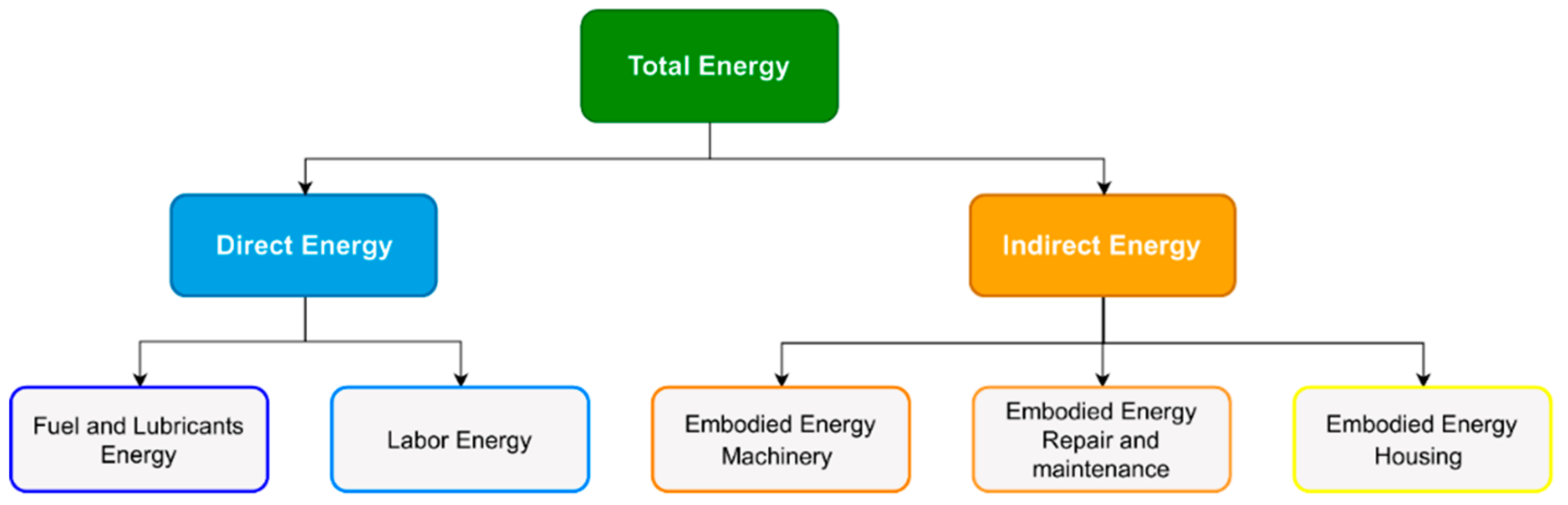
2.1. Energy Cost of Agricultural Operations

The execution of an agricultural operation requires both direct and indirect inputs. To that end, the employed approach in this study borrows from the well-established methodology of financial cost calculation [28], and allocates the total energy required to perform an operation to direct and indirect energy (Figure 1). The indirect energy concerns the energy assessment of inputs that are not related to the operation performed but concern the acquisition and the ownership of the equipment. The direct energy involves the energy assessment of the direct inputs related to agricultural operations.
On the basis of the above, the indirect energy is differentiated between the machinery and repair and maintenance embodied energy ( MJ · kg 1 ), as well as the housing embodied energy ( MJ · m 2 · y 1 ) . The machinery embodied energy refers to the energy required to manufacture the agricultural equipment [20,29]. The embodied energy of repair and maintenance can be either expressed as a percentage of the manufacturing energy requirements [30,31] or can be estimated in absolute numbers, as attempted by Mantoam et al. [32]. The housing embodied energy represents the energy contribution of all the building and infrastructure necessary for the storage of the equipment [30]. It should be noted that these denoted parameters are usually calculated for the entire life cycle of the machinery or building [33]. In this study, the energy contribution from manufacturing, repair and maintenance, and housing is reduced to the duration of the operation performed considering as related to the total life of the equipment.
The operation energy is divided into the fuel and lubricant energy ( MJ · l 1 ), and the embodied energy of labor ( MJ · h 1 ). The energy of fuels and lubricants is related to the fuel and lubricant consumption as calculated based on the ASABE (American Society of Agricultural and Biological Engineer) standards [34]. The embodied energy of labor expresses the energy consumed by the workers performing the operation [35]. Several approaches have been proposed in the literature regarding the estimation of the embodied energy of labor differing in the system boundaries and operations considered [16,36,37,38,39].

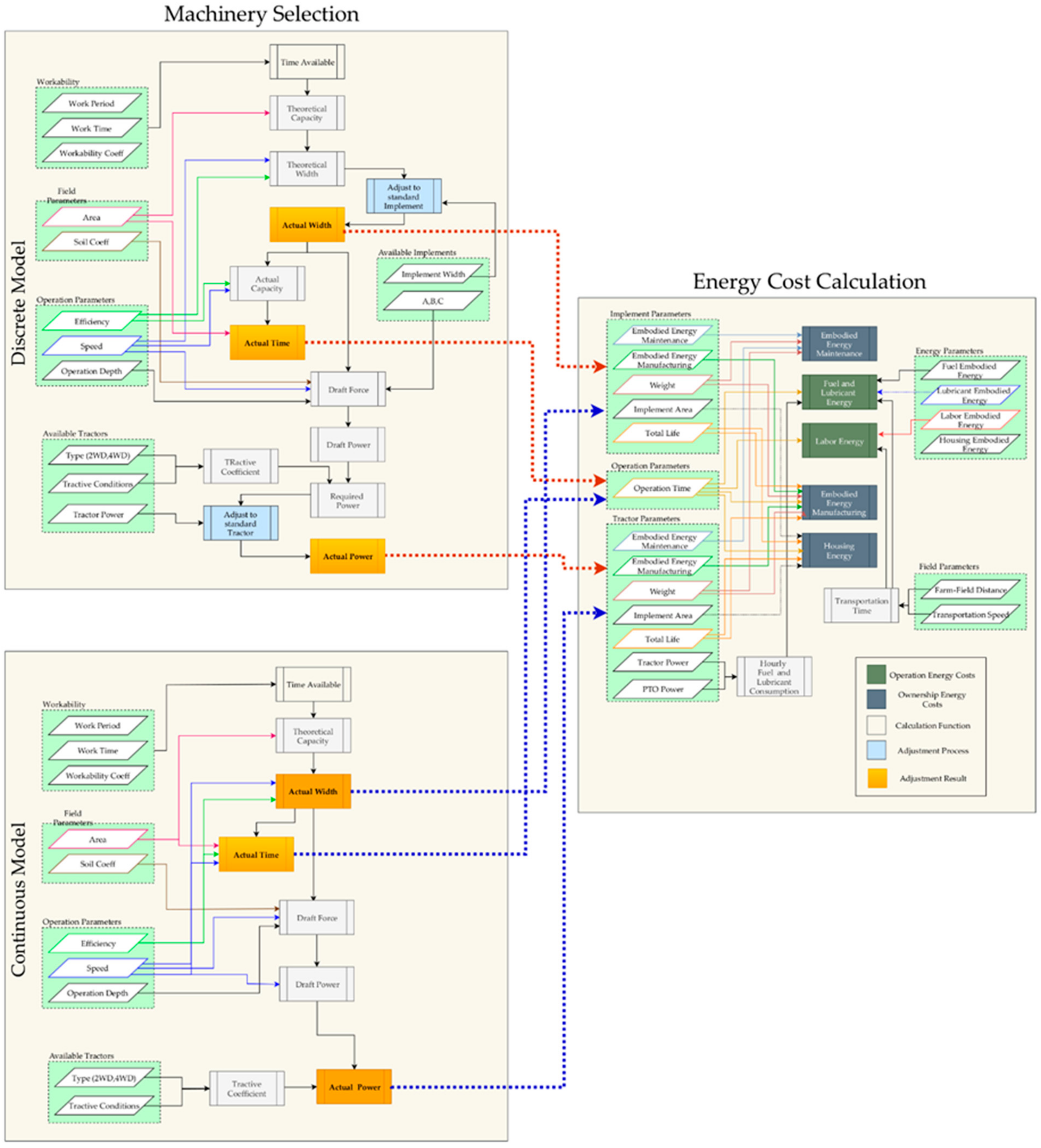
2.2. Energy Estimation Model

In order to calculate the energy cost of performing an agricultural operation, the model presented in Figure 2 was used. The calculation consists of two distinct stages, namely the machinery selection and the calculation of the energy costs. For the machinery selection stage, in order to estimate the effect of standardized machinery on the overall energy consumption, two models were considered, namely the continuous and the discrete model, while the energy cost calculation is the same for both models. The continuous model calculates the energy consumption of a theoretical machine system without correction to standard commercial machinery, while the discrete model considers the commercially available implements and tractors for the determination of the energy costs. More specifically, the necessary machine system (single or multiple if it is required) to perform the operation is automatically calculated by the model, considering both operational parameters and the machinery available. The calculation process of the discrete model is presented in detail below, however, the basic equations are standard for both models. Nevertheless, it should be highlighted that, in the continuous model, only a single machine system is considered.
During the machinery selection stage, first the available time t av ( h ) to perform an agricultural operation is calculated (Equation (1)):
t av = t wp · t wt · W coef
where t w p   d is the working period in days, t wt   h · d 1   is the working time, and W coef   is the workability coefficient [40]. Given a specific available time, the theoretical area capacity C th   m 2 · h 1 is calculated (Equation (2)):
C th = A t av
where A   m 2 is the size of the field under examination. The theoretical capacity determines, as a sequence, the theoretical minimum width w th   m (Equation (3)) that must be applied in order to complete the operation on time.
w th = C th E f   ·   s    
where E f   % stands for the efficiency of the operation performed, while s   km · h 1 is the operating speed.
Then, according to the discrete model, the theoretical width is adjusted based on the commercially available implements. When the theoretical width is smaller than the maximum width available, then the width selected is the one that is immediately bigger than the theoretical width. When the theoretical width is larger than the maximum width available, it means that more than one implements are required to perform the operation on time. In that case, the maximum width is selected (as many times as required), while the remaining width is adjusted to the next bigger available width. In should be noted that, in this step, the actual number of machines required to perform the operation is determined. Considering the above, the actual width w act   m of the operation performed is formulated and, as a consequence, the actual area capacity is calculated by Equation (4) as follows:
C act = w act · s · Ε f  
Finally, the actual duration of the operation is calculated (Equation (5)):
t act = A C act  
In the case of the continuous model where a correction to standard machines is not performed, the actual width and actual capacity are the same as the theoretical width and capacity and actual time coincides with the time available to perform the operation. Once the required implements have been determined, the calculation of the required tractors follows. The implement draft D draft   N is calculated according to the ASABE standards [41] by Equation (6):
D draft = F i · A + B · s + C · s 2 · w act · O depth  
where F i   ( ) is the soil texture adjustment parameter; A, B, and C are machine specific parameters; and O depth   cm is the operation depth. Considering the above, the draft power (kW) is calculated as follows [23]:
P draft = D draft   ·   s 1000  
Finally, the total power required P required   kW is calculated from Equation (8) as follows:
P required = P draft   Tr coef   ·   0.83  
where Tr coef   stands for the tractive coefficient [42], while the coefficient 0.83 is used for the Power Take Off (PTO) to gross-flywheel conversion [34]. The calculated P required   kW corresponds to the minimum power required to perform the operation considering the necessary implements as they were defined in the previous steps. However, commercial tractors are available with a standard power capacity for each model, as defined by the manufacturer. To that end, the required power is adjusted to the next bigger available. In the case of the continuous model, the required power coincides with the actual power because there is not a correction to standard tractors. The machinery selection stage provides the list of tractors-implements that are necessary for the completion of the procedure in the given time available for the discrete model and the single tractor and implement system for the continuous model. For each tractor-implement set, the energy costs of performing the operation are calculated.
Regarding the operation parameters calculations, the hourly fuel consumption F con   l · h 1 is calculated from Equation (9) (for diesel) as follows [34]:
F con = 2.64 · P ratio + 3.91 0.203   ·   738 · P ratio + 173 )   · P required  
where P ratio expresses the ratio of equivalent PTO power necessary for an operation to that maximum available from the PTO [34]. The relevant lubricant consumption L con l · h 1 is calculated in Equation (10) (for diesel) [34].
L con = 0.00059 · P required + 0.02169  
Lastly, it is important to note that, for the calculation of the operation energy costs, the transportation duration is also considered along with the operation duration. The resulting per hectare total energy En Tot   MJ is calculated as the sum of the direct En Direct and indirect energy En Indirect , as presented in Equation (11):
En Tot = En Direct + En Indirect
The direct energy En Direct   MJ is calculated by Equation (12) as follows:
En Direct = En Fuel + En Lubr + En Labor
where En Fuel (MJ) is the total fuel energy; En Lubr is the total lubricant energy and En Labor is the total labor energy expressed in Equations (13)–(15):
En Fuel = F con · t act · Emb Fuel
En Lubr = L con · t act · Emb Lubr
En Labor = t act · Emb Labor
where Emb Fuel   MJ · l 1 and Emb Lubr   MJ · l 1 are the embodied energy in the fuels and lubricants and Emb Labor ( MJ · h 1 ) is the per hour labor energy. With respect to the indirect energy consumption, Equation (16) applies as follows:
En Indirect = En Manufacturing + En RM + En Housing
The embodied energy for the manufacturing En Manufacturing   MJ of the equipment (tractor and implement) is expressed in Equation (17), reduced to total hours of the operation:
En Manufacturing = Emb Manufturing   ·   M h life   · t act  
where Emb Manufacturing   MJ · kg 1 is the embodied energy; M   kg is the mass of the tractor and the implement, respectively and h life   h is the total life hours of the machinery. The repair and maintenance embodied energy En RM   MJ , as already mentioned, is expressed as a percentage of the manufacturing energy requirements RM Rate (%) (Equation (18)):
En RM =   En Manufacturing   · RM Rate
Lastly, the housing energy En Housing (MJ) is calculated by Equation (19) reduced to total hours of the operation as follows:
En Housing =   Emb Housing   · A cover h life · t act
In that case, Emb Housing   MJ · m 2 · y 1 is the embodied energy of the facility required to house the equipment and A cover   m 2 is the area cover of each the machines (tractor or implement).

3. Case Study Description

The methodology described in the previous section was used to investigate the energy cost of performing two different tillage operations, considering different field areas and the available time window. The examined operations are secondary tillage performed by a field cultivator and deep tillage performed by a moldboard plow. Table 1 presents the operation parameters considered according to the ASABE standards [34]. The economic and total life is assumed to be identical for both implements. However, the operating speed differs with respect to the different operations because it depends on the operation depth, which is determined based on the general cultivation practices [43].
As mentioned in the methodology, the estimated required implement width and the tractor power are adjusted to fit with the next bigger commercially available one. To that effect, feature values of commercially available machinery were collected for the calculations as they are provided by the manufactures. These specifications include the width, weight and dimensions of the implements and the power, weight, and dimensions of the tractors. All the tractors (with power ranging from 37.4 kW to 456 kW) that were inserted in the model are 4WD, while the fuel type is diesel in all the cases examined. Regarding the calculation of the transportation energy cost, it is assumed that each field is located at a distance of 1 km from the farm. The tractor travels at 40 km   · h 1 and performs each trip once in order to complete the operation and return to the farm.
The embodied energy parameters considered for the model calculation are presented in Table 2. Various methodologies have been proposed for the calculation of the manufactured embodied energy of farm machinery; however, for the purposes of this study, the approach of Kitani et al. was selected [35]. With respect to the embodied energy of the maintenance of the machinery, it is calculated as a percentage of the respective manufacturing energy according to the approach of Aguilera et al. [30]. The approach of Aguilera et al. was also used for the estimation of the housing embodied energy, considering the average value per year and per spatial coverage of the service building. All the parameters presented in this section represent the input parameters of the calculation process of Figure 2, which are highlighted in the green boxes.

4. Results

This section presents the results of the implementation of the energy calculation tool with respect to the estimation of the machinery energy cost of performing three different tillage operations. Two different assessment models were examined, namely the discrete and the continuous model. The discrete model refers to the calculation of the required energy using the adjustment to standard commercial implements and tractors according to the process presented in the methodology. The continuous model refers to the theoretical energy consumption as it would be estimated without the adjustment to standard implement and standard values. The machinery selected in the latter case would have the exact performance characteristics with the estimated requirements to perform the operation. Furthermore, in that case, there are no maximum available values, indicating that the operation is performed with one set of tractor–implement, irrespective of the width and power necessary to operate within the time window available, which coincides with the actual operation time. The figures below present the total energy consumption, the total machine power, the number of machines, as well as the total operating width with reference to the time available and the cultivation area.

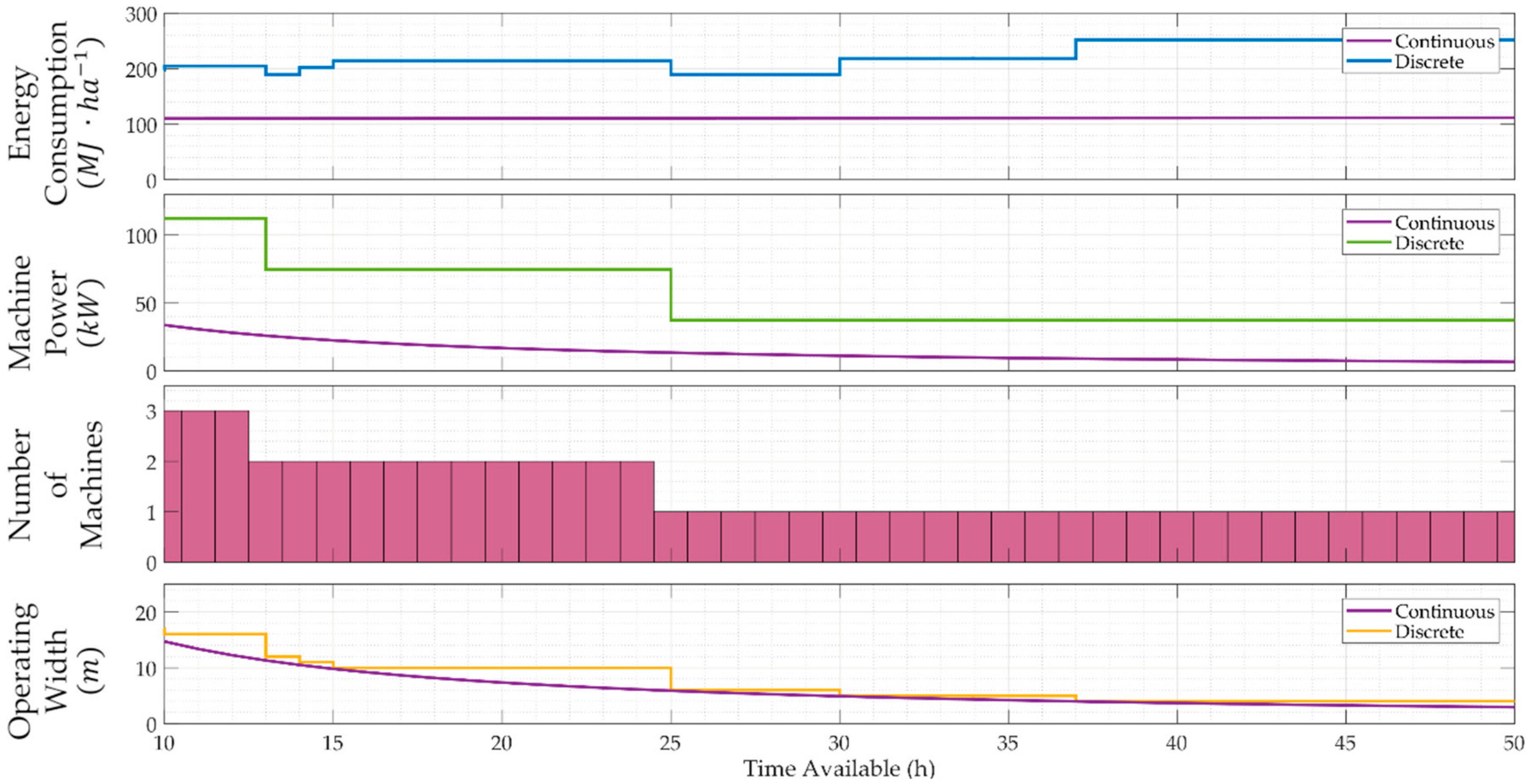
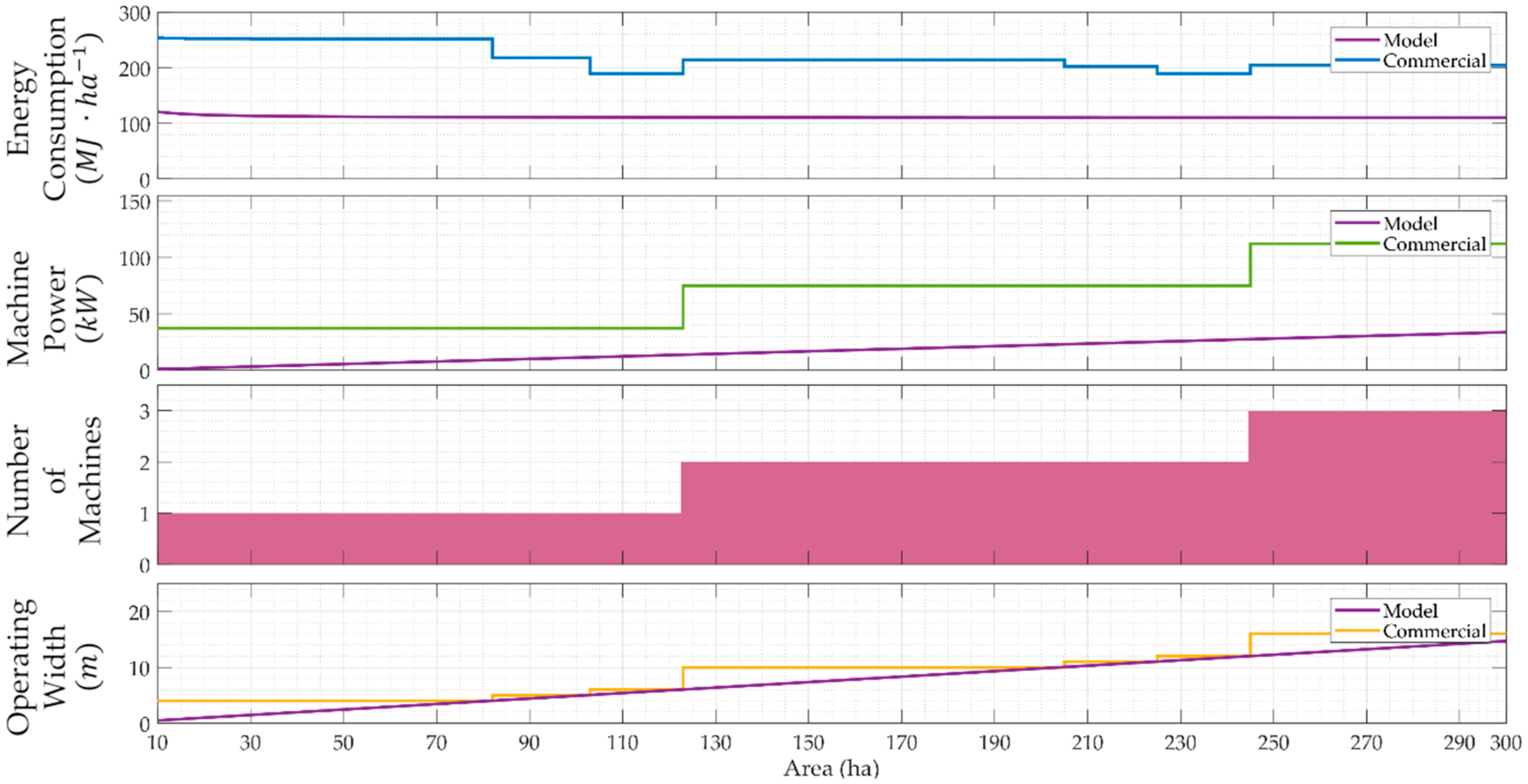
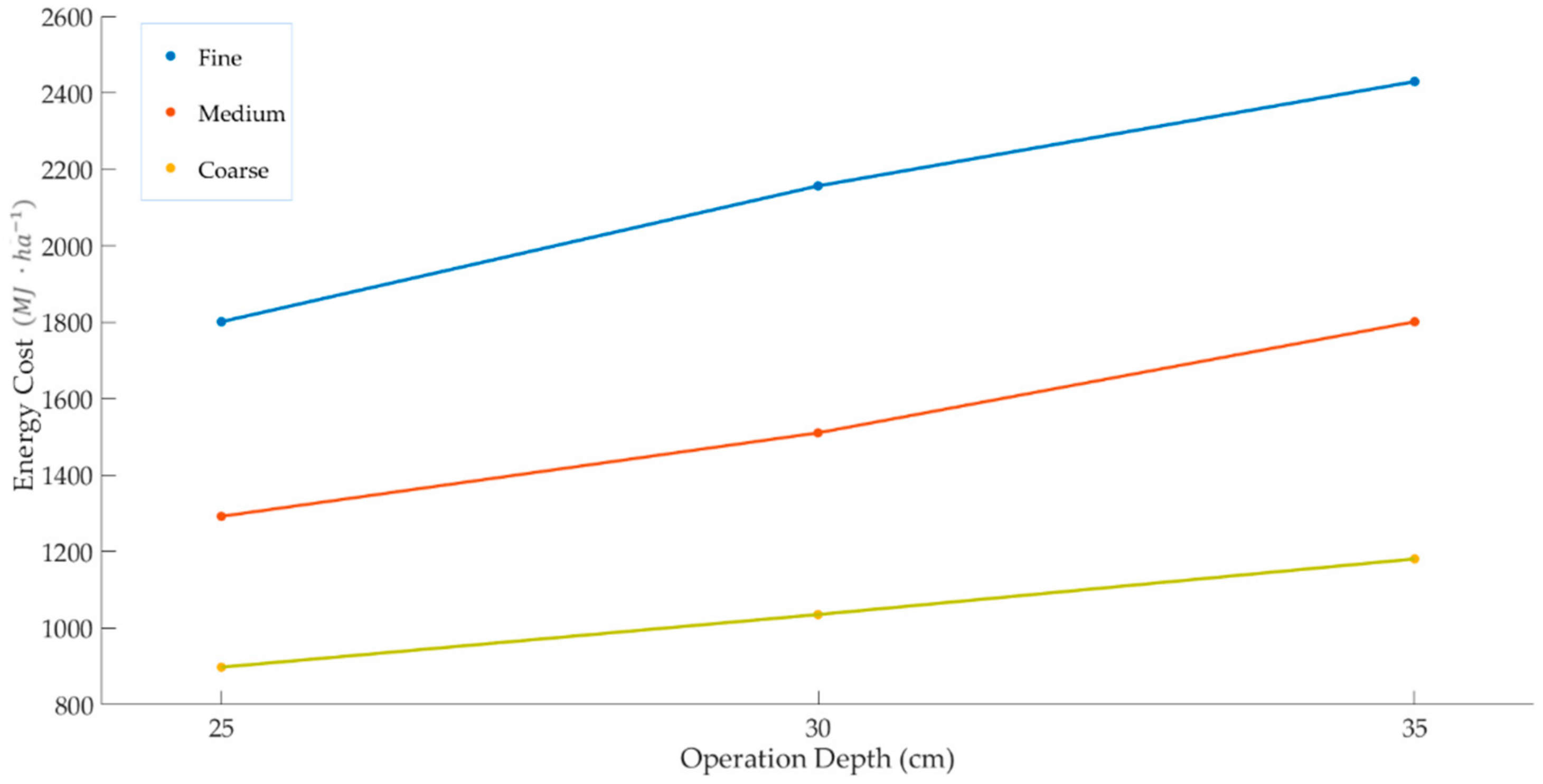
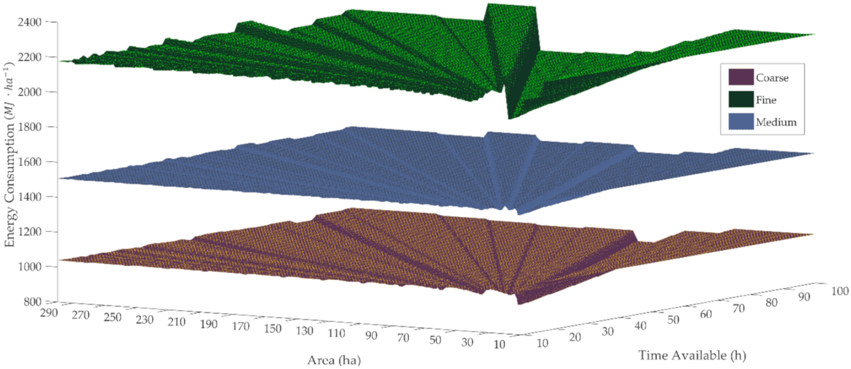
4.1. Field Cultivator

With respect to the secondary tillage with a field cultivator, Figure 3 presents the total energy cost, the total machine power, the number of machines, and the total operating width for cultivated areas of 100 ha in relation to the available time to perform the operation. The energy consumption for the specific area varies around the average value of 234.99 MJ · ha 1 . The tool selects the required machinery system to perform the operation within the available time window. As expected, the number of machines required to complete the operation decreases as the available time increases. For example, three machines are required to complete the operation in 10 h and two machines when the available time exceeds 13 h. After 25 h, only one machine is required to complete the operation and, as a result, only the required width decreases. The total energy consumed shows an upward trend owing to increased total operation time until the 37 h available time. At this point, only the smallest implement is used to complete the operation, and the time of operation does not change further with the energy consumed, being the same irrespective of the time available.
The discrete model represents the realistic approach for the calculation of the energy required to perform an operation. However, as presented in Figure 3, it is worth comparing it to the continuous model. In the case of field cultivator, the continuous model predicts an average energy cost of 111.83   MJ · ha 1 for the area of 100 ha, which is 2.1 times smaller than the respective discrete. The tractor power and the implement width that are actually used are significantly larger than those that are ideally required, resulting in increased energy consumption.
Figure 4 and Figure 5 present the energy cost and machinery requirements for completing the operation in 30 h and 50 h, respectively, in relation to the cultivated area. Little available time leads to a rapid increase of machinery needed, while in the case of more time availability, a second machine is required for fields larger than 200 ha. Considering that, for the field cultivator three, different implement options were available (4 m, 5 m, and 6 m), the operating width increases after an area of 135 ha for an available time of 50 h. The energy consumed shows a downwards trend when increasing the cultivated area, with average values of 218.94   MJ · ha 1 for 30 h and 228.98   MJ · ha 1 for 50 h available time. The average energy consumed increases when increasing the available time because the operating time increases as well. In the case of 50 h available, the energy consumed per hectare remains constant for fields between 2 and 135 ha with the given implements, as the smallest implement can cover this area without requiring a second one to perform the operation timely.
In order to gain full insight regarding the formulation of the model, Figure 6 presents the results for the time available and the area, ranging from 10 h to 100 h and from 10 ha to 300 ha, respectively. The discrete model estimates a higher energy consumption per ha than the continuous model. The only exception is the area of 1 ha, where the continuous model is more energy consuming than the discrete model after approximately 40 h of time available owing to the very small stipulated operating width. However, as such a small operating width is not realistic (approximately 0.015 m for 1 ha and 100 h available time), energy values corresponding to areas below 10 ha were discarded from Figure 6. The total average energy cost is 226.51   MJ · ha 1 for the discrete model, which is 1.98 times higher than the continuous model. For the field cultivator, 69.4% of energy consumption derives from the operation of the machinery, while 30.6% is attributed to its ownership.

4.2. Moldboard Plow

Figure 7 presents the total energy consumption of performing primary tillage with a moldboard plow in a field of 100ha in relation to the time available to perform the operation. The average energy consumption for the 100 ha is 1505.82   MJ · ha 1 for the discrete model. It is observed that the continuous model shows higher energy consumption, approximately 1.06 times, than the discrete model demonstrating the effect of the operation depth and type in the overall energy costs.
The required width and power to complete the operation on time do not differ significantly between the discrete and the continuous model. This can be attributed to the large energy requirements of the operation, as well as to the availability of implements. In the case of the moldboard plow, the commercially available width of the implements presented more subdivisions in the range of 1.1–4.4 m, providing the tool with more options during the machinery selection stage.
Figure 8 presents the evolution of the model with respect to the field area, considering time available of 50 h. For field areas up to 30 ha, the operation can be performed with one tractor carrying the minimum available implement (1.1 m). From this point, the implement width is further increased until it reaches the maximum available of 4.4 m. Then, with a further increase in the area, a second machine is needed to perform the operation timely. The width and power increasing pattern is the same for the second machinery as previously described until the point when a third machine is required. The average energy cost, in the case of 50 h of available time, is 1508.61   MJ · ha 1 .
The total energy consumption of the discrete and continuous model for moldboard plowing in a wide range of area and available time is presented in Figure 9. The continuous model has an average energy cost of 1604.95   MJ · ha 1 , which is 1.06 times higher than the discrete model, which presents an average energy cost per hectare of 1510.37   MJ · ha 1 . This finding highlights the importance of time when performing an agricultural operation of high operation energy requirements. For moldboard plowing, 90.4% of the energy consumed is attributed to operation, while only 9.6% of the energy consumed refers to the energy ownership costs. As a consequence, the adjustment to the closest bigger available implement resulted in a reduction of the total energy, as the actual time required to perform the operation decreased with the increased implements’ width.

5. Discussion

In the previous section, the energy cost of performing secondary tillage with a field cultivator and primary tillage with a moldboard plow was presented. The results concerned tillage on medium soil with an operation depth of 15 cm and 30 cm, respectively. Tillage with a moldboard plow was calculated to be 6.67 times more energy consuming than field cultivation, which is an outcome that is expected considering the depth and the nature of the operation. For the field cultivator, the indirect energy costs account for almost 1/3 of the total energy consumed, while for the moldboard plow, only for 1/10. The direct energy cost is the determining factor of the total energy consumption. However, it is worth noting that its contribution to the total energy consumed increases as the energy intensity of the operation increases. Nevertheless, it should be stated that the available time to perform an operation and the different field areas do not seem to strongly affect the total energy per hectare.
Regarding machinery selection, the method employed focuses on the available time for field operations rather than the assessment of the financial cost of the equipment. In that light, the dimensioning of the implement requires sufficient power in the tractor as a prerequisite for the execution of the operation on time. The main disadvantage of the method is the fact that the operating economic costs are not considered during the selection stage. Additionally, the tool is designed in order to facilitate machinery selection, taking into account technical conditions rather than economic ones. As a consequence, a selection of the machinery system by applying this method can lead to non-optimum solutions in terms of economic criteria such as minimum operating or ownership cost. Furthermore, it is of limited use in cases where the equipment has already been purchased.
Τhe results indicate that the proper allocation of tools and tractors and the use of the appropriate combination of machinery in each operation can affect the total energy consumed. In the case of light soil cultivation (field cultivator), the total energy consumed is higher than that expected from model calculations owing to the use of larger implements than those required to perform the operation on time. On the other hand, in the case of the moldboard plow, the use of a larger implement than the one required to perform the operation on time leads to a decreased energy consumption, which is justified when considering the contribution of the operation cost to the total energy cost of this operation. Nevertheless, the availability and the subdivision of the implement width strongly affect the diversion from the model consumption calculated for the examined cases.
Another factor that was examined was the sensitivity of the energy consumed with respect to the type of soil and the operation depth. In that end, the calculations were performed for different depths (plus 5 cm and minus 5 cm from the original example), as presented in Figure 10, and soil types (fine and coarse in addition to medium soil), as presented in Figure 11. For the field cultivator, it was found that the operation depth and the type of soil do not affect the total energy consumed in the case of the discrete model. This is attributed to the fact that the minimum available commercial machinery covers the requirements of the operation, irrespective of the type of soil or the depth.
However, in the case of moldboard plowing, both the operation depth and the type of soil strongly influence the total energy consumed. As presented in Figure 10, the energy consumed for deep tillage in fine soil is almost two times higher than the that for coarse soil in the case of an operation depth of 25 cm. Additionally, in the case of fine soil, the energy for performing the operation at an operation depth of 35 cm is 2429.54   MJ · ha 1 , 1.35 times higher than when performing it at a depth of 25 cm (1800.88   MJ · ha 1 ).

6. Conclusions

The assessment and management of agricultural production is a multivariate problem. Thereby, the introduction and use of operation management tools can contribute towards the effective management of agricultural production and the quantification of its environmental impact. Existing tools and methodologies in most cases examine the entire life cycle of the cultivation or focus on the use of plant protection products and fertilizers owing to their proven severe adverse impact compared with the other agricultural inputs. Nevertheless, the quantification of the contribution of machinery to the total energy consumed is important and constitutes an essential first step for the evaluation of alternative technologies and tools. In fact, the results highlight the benefits of optimal allocation of tools, especially in the task of light soil cultivation, where the energy consumed using the commercially available machinery (226.51   MJ · ha 1 ) is almost double the optimal energy expressed by the continuous model (113.88   MJ · ha 1 ).
This paper attempted to examine and set the base of evaluating the energy consumption considering various operational parameters coupled with the commercial availability of implements and tractors. The model selects (from a collection of available implements and tractors) the required machinery to perform the operation in a given time, while evaluating the resulting energy cost. Even though the available time and the cultivated area do not seem to strongly affect the energy consumption per hectare, the commercially available implements highly affect the total energy cost. From the examined case studies, the effect of using unsuitable equipment was highlighted, indicating a promising potential for further reduction in the energy consumed from the machinery. Towards this direction, future work incorporating the consideration of financial parameters during the machinery selection is required in order to assess the economic and environmental performance of the machinery in an integrated manner.

Author Contributions

Conceptualization, M.L., D.K., C.G.S., and D.B.; data curation, D.K. and D.B; formal analysis, D.K.; investigation, M.P. and D.K.; methodology, M.L. and D.K.; software, M.L.; supervision, D.B.; validation, D.K., C.G.S., and D.B.; writing—original draft, M.L.; writing—review and editing, D.K., C.G.S., and D.B. All authors have read and agreed to the published version of the manuscript.

Funding

The work was supported by the project “Research Synergy to address major challenges in the nexus: energy-environment-agricultural production (Food, Water, Materials)” NEXUS, funded by the Greek Secretariat for Research and Technology (GSRT), Pr. No. MIS 5002496.

Conflicts of Interest

The authors declare no conflict of interest.

References

  1. De Olde, E.M.; Moller, H.; Marchand, F.; McDowell, R.W.; MacLeod, C.J.; Sautier, M.; Halloy, S.; Barber, A.; Benge, J.; Bockstaller, C.; et al. When experts disagree: The need to rethink indicator selection for assessing sustainability of agriculture. Environ. Dev. Sustain. 2017, 19, 1327–1342. [Google Scholar] [CrossRef] [Green Version]
  2. Bockstaller, C.; Beauchet, S.; Manneville, V.; Amiaud, B.; Botreau, R. A tool to design fuzzy decision trees for sustainability assessment. Environ. Model. Softw. 2017, 97, 130–144. [Google Scholar] [CrossRef]
  3. Rodias, E.C.; Lampridi, M.; Sopegno, A.; Berruto, R.; Banias, G.; Bochtis, D.D.; Busato, P. Optimal energy performance on allocating energy crops. Biosyst. Eng. 2019, 181, 11–27. [Google Scholar] [CrossRef]
  4. Lampridi, M.G.; Sørensen, C.G.; Bochtis, D.D. Agricultural Sustainability: A Review of Concepts and Methods. Sustainability 2019, 11, 5120. [Google Scholar] [CrossRef] [Green Version]
  5. Bockstaller, C.; Guichard, L.; Keichinger, O.; Girardin, P.; Galan, M.B.; Gaillard, G. Review article Comparison of methods to assess the sustainability of agricultural systems. A review. Agronomy 2009, 29, 223–235. [Google Scholar]
  6. Snapp, S.S.; Grabowski, P.; Chikowo, R.; Smith, A.; Anders, E.; Sirrine, D.; Chimonyo, V.; Bekunda, M. Maize yield and profitability tradeoffs with social, human and environmental performance: Is sustainable intensification feasible? Agric. Syst. 2018, 162, 77–88. [Google Scholar] [CrossRef]
  7. Allahyari, M.S.; Daghighi Masouleh, Z.; Koundinya, V. Implementing Minkowski fuzzy screening, entropy, and aggregation methods for selecting agricultural sustainability indicators. Agroecol. Sustain. Food Syst. 2016, 40, 277–294. [Google Scholar] [CrossRef]
  8. De Olde, E.M.; Oudshoorn, F.W.; Sørensen, C.A.G.; Bokkers, E.A.M.; De Boer, I.J.M. Assessing sustainability at farm-level: Lessons learned from a comparison of tools in practice. Ecol. Indic. 2016, 66, 391–404. [Google Scholar] [CrossRef]
  9. Sajjad, H.; Nasreen, I. Assessing farm-level agricultural sustainability using site-specific indicators and sustainable livelihood security index: Evidence from Vaishali district, India. Community Dev. 2016, 47, 602–619. [Google Scholar] [CrossRef]
  10. Gaviglio, A.; Bertocchi, M.; Demartini, E. A Tool for the Sustainability Assessment of Farms: Selection, Adaptation and Use of Indicators for an Italian Case Study. Resources 2017, 6, 60. [Google Scholar] [CrossRef]
  11. Peano, C.; Migliorini, P.; Sottile, F. A methodology for the sustainability assessment of agri-food systems. Ecol. Soc. 2014, 19, 19. [Google Scholar] [CrossRef] [Green Version]
  12. Chopin, P.; Tirolien, J.; Blazy, J.M. Ex-ante sustainability assessment of cleaner banana production systems. J. Clean. Prod. 2016, 139, 15–24. [Google Scholar] [CrossRef]
  13. De Luca, A.I.; Falcone, G.; Stillitano, T.; Iofrida, N.; Strano, A.; Gulisano, G. Evaluation of sustainable innovations in olive growing systems: A Life Cycle Sustainability Assessment case study in southern Italy. J. Clean. Prod. 2018, 171, 1187–1202. [Google Scholar] [CrossRef]
  14. Rodias, E.; Berruto, R.; Bochtis, D.; Busato, P.; Sopegno, A. A computational tool for comparative energy cost analysis of multiple-crop production systems. Energies 2017, 10, 831. [Google Scholar] [CrossRef]
  15. Bartzas, G.; Vamvuka, D.; Komnitsas, K. Comparative life cycle assessment of pistachio, almond and apple production. Inf. Process. Agric. 2017, 4, 188–198. [Google Scholar] [CrossRef]
  16. Strapatsa, A.V.; Nanos, G.D.; Tsatsarelis, C.A. Energy flow for integrated apple production in Greece. Agric. Ecosyst. Environ. 2006, 116, 176–180. [Google Scholar] [CrossRef]
  17. Rodias, E.; Berruto, R.; Bochtis, D.; Sopegno, A.; Busato, P. Green, yellow, and woody biomass supply-chain management: A review. Energies 2019, 12, 3020. [Google Scholar] [CrossRef] [Green Version]
  18. Viola, I.; Marinelli, A. Life Cycle Assessment and Environmental Sustainability in the Food System. Agric. Agric. Sci. Procedia 2016, 8, 317–323. [Google Scholar] [CrossRef] [Green Version]
  19. Mantoam, E.J.; Romanelli, T.L.; Gimenez, L.M.; Milan, M. Energy demand and greenhouse gases emissions in the life cycle of coffee harvesters. Chem. Eng. Trans. 2017, 58, 175. [Google Scholar]
  20. Mantoam, E.J.; Romanelli, T.L.; Gimenez, L.M. Energy demand and greenhouse gases emissions in the life cycle of tractors. Biosyst. Eng. 2016, 151, 158–170. [Google Scholar] [CrossRef]
  21. Sørensen, C.G.; Halberg, N.; Oudshoorn, F.W.; Petersen, B.M.; Dalgaard, R. Energy inputs and GHG emissions of tillage systems. Biosyst. Eng. 2014, 120, 2–14. [Google Scholar] [CrossRef]
  22. Tassielli, G.; Renzulli, P.A.; Mousavi-Avval, S.H.; Notarnicola, B. Quantifying life cycle inventories of agricultural field operations by considering different operational parameters. Int. J. Life Cycle Assess. 2019, 24, 1075–1092. [Google Scholar] [CrossRef]
  23. Bochtis, D.; Sorensen, C.G.; Kateris, D. Operations Management in Agriculture, 1st ed.; Elsevier: Amsterdam, The Netherlands, 2018; ISBN 9780128097168. [Google Scholar]
  24. Edwards, W. Farm Machinery Selection. Available online: https://www.extension.iastate.edu/agdm/crops/html/a3-28.html (accessed on 3 January 2020).
  25. Bochtis, D.D.; Sørensen, C.G.C.; Busato, P. Advances in agricultural machinery management: A review. Biosyst. Eng. 2014, 126, 69–81. [Google Scholar] [CrossRef]
  26. Marinoudi, V.; Sørensen, C.G.; Pearson, S.; Bochtis, D. Robotics and labour in agriculture. A context consideration. Biosyst. Eng. 2019, 184, 111–121. [Google Scholar] [CrossRef]
  27. Sørensen, C.G.; Nielsen, V. Operational analyses and model comparison of machinery systems for reduced tillage. Biosyst. Eng. 2005, 92, 143–155. [Google Scholar] [CrossRef]
  28. Lampridi, M.G.; Kateris, D.; Vasileiadis, G.; Marinoudi, V.; Pearson, S.; Sørensen, C.G.; Balafoutis, A.; Bochtis, D. A Case-Based Economic Assessment of Robotics Employment in Precision Arable Farming. Agronomy 2019, 9, 175. [Google Scholar] [CrossRef] [Green Version]
  29. Lee, J.; Cho, H.J.; Choi, B.; Sung, J.; Lee, S.; Shin, M. Life cycle assessment of tractors. Int. J. Life Cycle Assess. 2000, 5, 205–208. [Google Scholar] [CrossRef]
  30. Aguilera, E.; Guzmán, G.I.; Infante-amate, J.; García-ruiz, R.; Herrera, A.; Villa, I. Embodied energy in agricultural inputs. Incorporating a historical perspective. DT-SEHA 15. 2015, p. 119. Available online: http://hdl.handle.net/10234/141278 (accessed on 5 December 2019).
  31. Audsley, E.; Stacey, K.; Parsons, D.J.; Williams, A.G. Estimation of the greenhouse gas emissions from agricultural pesticide manufacture and use. Uma ética para quantos? 2014, p. 20. Available online: https://dspace.lib.cranfield.ac.uk/bitstream/handle/1826/3913/Estimation_of_the_greenhouse_gas_emissions_from_agricultural_pesticide_manufacture_and_use2009.pdf;jsessionid=DC4D51F03A8C73E065940B464D68BDBD?sequence=1 (accessed on 5 December 2019).
  32. Mantoam, E.J.; Mekonnen, M.M.; Romanelli, T.L. Energy demand and water footprint study of an agricultural machinery industry. Agric. Eng. Int. CIGR J. 2018, 20, 132. [Google Scholar]
  33. Kitani, O. CIGR Handbook of Agricultural Engineering, Volume 5: Energy and Biomass Engineering; American Society of Agricultural and Biological Engineers: St. Joseph, MI, USA, 1999. [Google Scholar]
  34. ASABE. ASAE D497.5 FEB 2006 Agricultural Machinery Management Data; ASABE: St. Joseph, MI, USA, 2006. [Google Scholar]
  35. Kitani, O.; Jungbluth, T.; Peart, R.; Ramdani, A. CIGR Handbook of Agricultural Engineering Volume V; CIGR: Liege, Belgium, 1999; ISBN 0929355970. [Google Scholar]
  36. Canakci, M.; Akinci, I. Energy use pattern analyses of greenhouse vegetable production. Energy 2006, 31, 1243–1256. [Google Scholar] [CrossRef]
  37. Kuswardhani, N.; Soni, P.; Shivakoti, G.P. Comparative energy input-output and financial analyses of greenhouse and open field vegetables production in West Java, Indonesia. Energy 2013, 53, 83–92. [Google Scholar] [CrossRef]
  38. Reineke, H.; Stockfisch, N.; Märländer, B. Analysing the energy balances of sugar beet cultivation in commercial farms in Germany. Eur. J. Agron. 2013, 45, 27–38. [Google Scholar] [CrossRef]
  39. Schramski, J.R.; Jacobsen, K.L.; Smith, T.W.; Williams, M.A.; Thompson, T.M. Energy as a potential systems-level indicator of sustainability in organic agriculture: Case study model of a diversified, organic vegetable production system. Ecol. Model. 2013, 267, 102–114. [Google Scholar] [CrossRef]
  40. Busato, P.; Berruto, R. Minimising manpower in rice harvesting and transportation operations. Biosyst. Eng. 2016, 151, 435–445. [Google Scholar] [CrossRef]
  41. ASABE. D497.7: Agricultural Machinery Management Proposed; ASABE: St. Joseph, MI, USA, 2015. [Google Scholar]
  42. ASAE. ASAE EP496.3—Agricultural Machinery Management; ASABE: St. Joseph, MI, USA, 2009. [Google Scholar]
  43. Tsatsarelis, C. Agricultural Machinery Management, 1st ed.; Giachoudi Publications: Thessaloniki, Greece, 2006; ISBN 960-7425-86-3. [Google Scholar]
  44. Saunders, C.; Barber, A.; Taylor, G. Food Miles-Comparative Energy/Emissions Performance of New Zealand’s Agriculture Industry; Agribusiness and Economics Research Unit, Lincoln University: Canterbury, New Zealand, 2006. [Google Scholar]
Figure 1. Energy costs of agricultural operations.
Energies 13 00769 g001
Figure 2. Calculation model.
Energies 13 00769 g002
Figure 3. Energy consumption, machine power, number of machines, and operating width for a cultivated area of 100 ha (field cultivator).
Energies 13 00769 g003
Figure 4. Energy consumption, machine power, number of machines, and operating width for 30 h time available (field cultivator).
Energies 13 00769 g004
Figure 5. Energy consumption, machine power, number of machines, and operating width for 50 h time available (field cultivator).
Energies 13 00769 g005
Figure 6. Energy consumption model for the field cultivator.
Energies 13 00769 g006
Figure 7. Energy consumption, machine power, number of machines, and operating width for a cultivated area of 100 ha (moldboard plow).
Energies 13 00769 g007
Figure 8. Energy consumption, machine power, number of machines, and operating width for 50 h time available (field cultivator).
Energies 13 00769 g008
Figure 9. Energy consumption model for moldboard plow.
Energies 13 00769 g009
Figure 10. Moldboard plow energy consumption for various soil types and operation depths.
Energies 13 00769 g010
Figure 11. Moldboard plow energy consumption discrete model for various soil types.
Energies 13 00769 g011
Table 1. Operation input parameters.
UnitsMoldboard PlowField Cultivator
Implement Parameters A, B, and C 1-652-0-5.132-1.9-0
Economic Life 1y1515
Total Life 1 h20002000
Efficiency 1 %8085
Operating Speed 1 km · h 1 78
Operating Depth 2cm3015
Soil Coefficient (Medium Soil) 1 -0.70.85
Implement Width Range *m1.1–4.44–6
1 [34], 2 [43] * Commercial values.
Table 2. Energy parameters.
Energy ParameterUnitsValue
Tractor Embodied Energy (Manufacturing) 1 MJ · kg 1 138
Implement Embodied Energy (Manufacturing) 1 MJ · kg 1 180
Tractor Embodied Energy (Maintenance) 2%45
Implement Embodied Energy (Maintenance) 2%30
Labor Embodied Energy 3 MJ · h 1 2.2
Fuel Embodied Energy (Diesel) 1 MJ · l 1 47.8
Lubricant Embodied Energy 4 MJ · l 1 46
Housing Embodied Energy 2 MJ · m 2 · y 1 21
1 [33], 2 [30], 3 [16], 4 [44].

