Real-Time Control Strategy for Aggregated Electric Vehicles to Smooth the Fluctuation of Wind-Power Output


Abstract
:1. Introduction
2. The Control Framework of Aggregated Electric Vehicles (EVs) Participating in Power Grid Scheduling
- (1)
- Do not participate in grid scheduling. An EV not subject to the schedule in the charging process. When the EV is connected to the charging pile, it is immediately charged at the rated maximum charging power until the EV leaves the charging pile or the EV battery reaches the set target value.
- (2)
- Participate in grid scheduling but not allowed to discharge to grid. This process can be called grid-to-vehicle (G2V).
- (3)
- Participate in grid scheduling and allow discharge to the vehicle. This process can be called vehicle-to-grid (V2G).
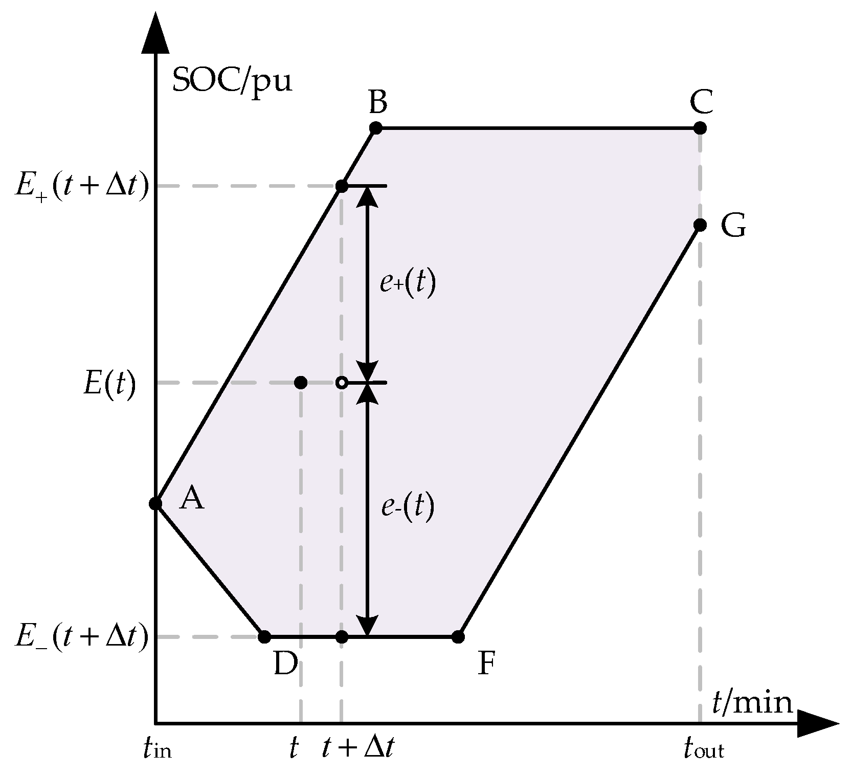
3. The Charging/Discharging Energy Boundary Model of EVs
4. Wind-Power Fluctuation Smoothing Strategy of Aggregated EVs in Real Time
4.1. Tracking Target of the Total Charging Power of the Aggregated EVs
4.2. The Power Allocation Method of Aggregated EVs
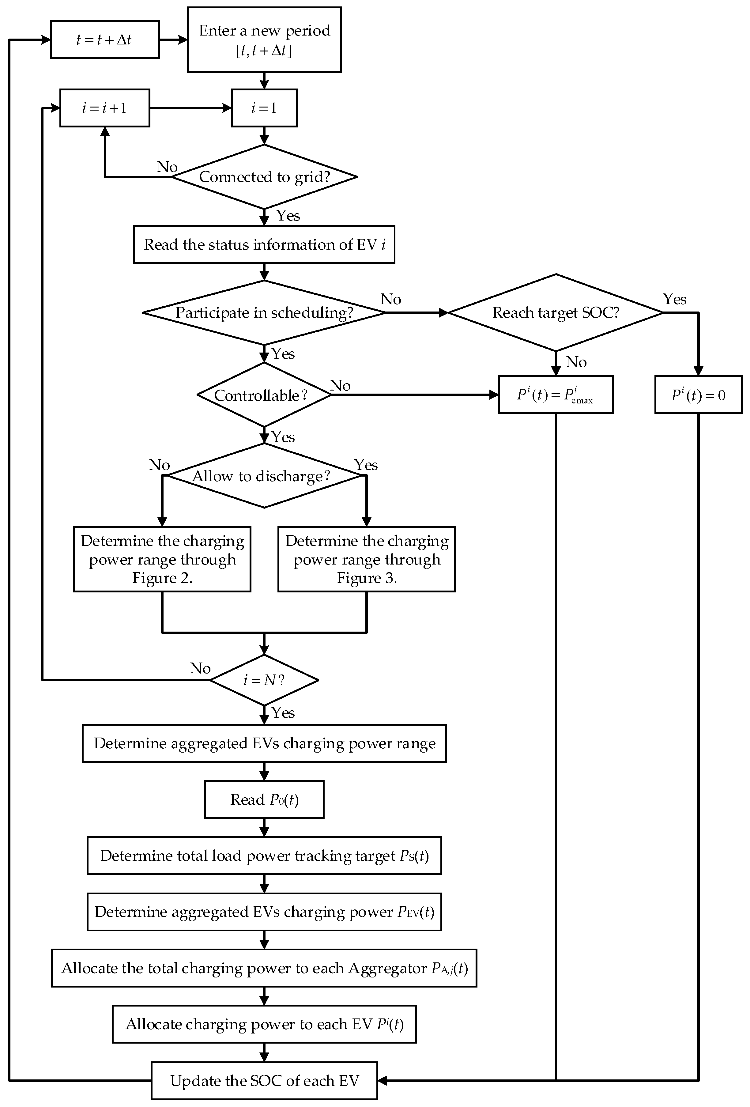
4.3. Real-Time Control Flow for Aggregated EVs
5. Case Analysis
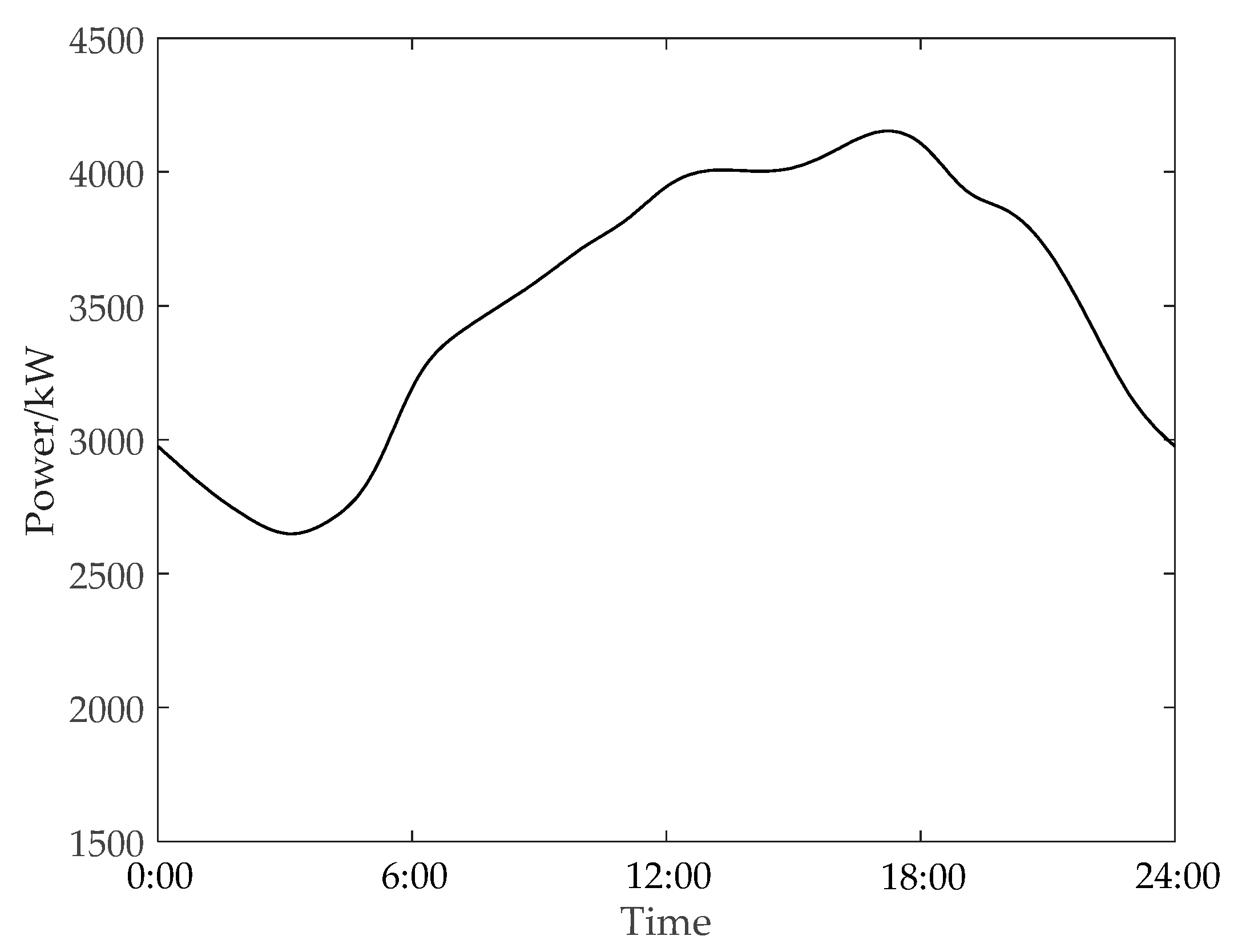
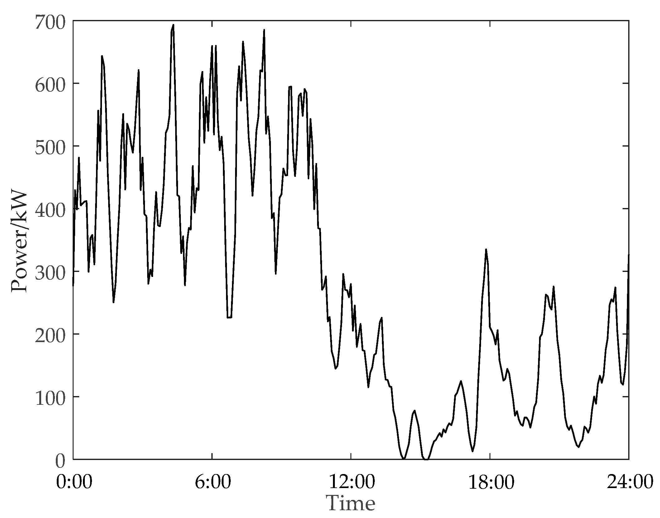
5.1. Case Data
5.2. Results Analysis
5.2.1. Results of Real-Time Control Strategy for Aggregated EVs to Smooth Wind Power Fluctuation
5.2.2. Analysis of the Influence of the Filter Time Constant on Smoothing Effect
5.2.3. Analysis of the Influence of the Proportion of EVs in Vehicle-to-Grid (V2G) Mode on Smoothing Effect
6. Conclusions
Author Contributions
Funding
Conflicts of Interest
Appendix A
Charging Demand Simulation Method Based on Trip Chain
- (1)
- tin_i: arrival time of the i-th trip destination;
- (2)
- tout_i: leaving time of the i-
- (3)
- th destination;
- (4)
- Tx(i-1,i): the driving duration between the (i−1)-th destination and i-th destination;
- (5)
- Tp_i: the parking duration at the i-th destination.
- (1)
- {Dk|k = 1,2,…,U}(U is the total number of destination types): destination type collection, and type (i) = Dk indicates that the type of the i-th destination is Dk;
- (2)
- d(i-1,i): the trip mileage between the (i−1)-th destination and i-th destination.


| No. | First Charge | Second Charge | No. | First Charge | Second Charge | ||||
|---|---|---|---|---|---|---|---|---|---|
| On-Grid Time | Off-Grid Time | On-Grid Time | Off-Grid Time | On-Grid Time | Off-Grid Time | On-Grid Time | Off-Grid Time | ||
| 1 | 6:55 | 16:38 | 19:50 | ↓7:36 | 76 | 8:32 | 17:20 | ||
| 2 | ↑17:28 | 7:15 | 20:49 | ↓8:32 | 77 | ↑16:59 | 8:47 | 19:10 | ↓7:57 |
| 3 | ↑15:50 | 8:26 | 18:51 | ↓7:41 | 78 | ↑18:58 | 7:57 | 18:18 | ↓8:50 |
| 4 | ↑15:48 | 7:22 | 19:15 | ↓7:15 | 79 | ↑16:31 | 7:37 | 17:32 | ↓6:18 |
| 5 | ↑21:01 | 7:53 | 21:00 | ↓7:14 | 80 | ↑19:20 | 6:17 | 20:53 | ↓7:38 |
| 6 | ↑17:40 | 9:22 | 13:13 | 20:49 | 81 | ↑18:32 | 7:11 | ||
| 7 | 17:36 | ↓8:19 | 82 | ↑19:12 | 6:34 | 19:06 | ↓6:54 | ||
| 8 | 17:49 | ↓7:20 | 83 | ↑19:54 | 9:08 | 17:31 | ↓9:02 | ||
| 9 | ↑20:49 | 8:12 | 18:14 | ↓8:28 | 84 | ↑19:48 | 5:48 | ||
| 10 | 12:55 | 15:47 | 20:30 | ↓7:29 | 85 | ↑15:40 | 5:48 | 18:17 | ↓7:59 |
| 11 | 11:18 | 17:16 | 86 | ↑19:51 | 9:11 | 20:29 | ↓7:13 | ||
| 12 | 21:05 | ↓7:30 | 87 | ↑19:21 | 6:11 | ||||
| 13 | ↑16:22 | 8:02 | 17:29 | ↓8:11 | 88 | 8:31 | 13:40 | ||
| 14 | 17:05 | ↓7:44 | 89 | ↑15:21 | 8:29 | 17:00 | ↓5:38 | ||
| 15 | 13:35 | 19:01 | 90 | ↑15:39 | 7:35 | 21:14 | ↓5:54 | ||
| 16 | 16:47 | ↓6:58 | 91 | 9:48 | 15:58 | ||||
| 17 | 9:09 | 17:17 | 19:54 | ↓5:28 | 92 | 8:25 | 14:40 | ||
| 18 | 15:59 | ↓10:16 | 93 | ↑17:43 | 8:09 | 22:05 | ↓5:38 | ||
| 19 | ↑17:50 | 9:14 | 16:44 | ↓8:21 | 94 | 20:52 | ↓7:04 | ||
| 20 | 8:50 | 16:18 | 95 | 9:00 | 14:21 | ||||
| 21 | 13:15 | 19:03 | 96 | 20:29 | ↓8:34 | ||||
| 22 | ↑17:07 | 5:12 | 13:06 | 17:53 | 97 | ↑20:20 | 4:15 | ||
| 23 | ↑20:02 | 5:50 | 98 | 8:43 | 18:23 | ||||
| 24 | ↑18:40 | 9:26 | 16:01 | ↓7:35 | 99 | ↑18:14 | 6:50 | 16:59 | ↓10:19 |
| 25 | 10:29 | 19:32 | 100 | ↑18:23 | 8:52 | 17:02 | ↓6:06 | ||
| 26 | ↑17:25 | 8:38 | 18:55 | ↓9:45 | 101 | ↑17:31 | 5:33 | 18:11 | ↓9:59 |
| 27 | ↑16:18 | 9:57 | 17:32 | ↓9:23 | 102 | 19:44 | ↓7:19 | ||
| 28 | 9:37 | 14:21 | 103 | 5:47 | 14:42 | ||||
| 29 | 7:17 | 16:45 | 104 | 9:31 | 15:06 | ||||
| 30 | ↑17:08 | 7:56 | 18:16 | ↓9:52 | 105 | ↑18:29 | 8:05 | 19:23 | ↓7:00 |
| 31 | ↑19:04 | 4:41 | 19:01 | ↓10:52 | 106 | ↑18:07 | 10:14 | ||
| 32 | ↑19:25 | 6:44 | 13:10 | 17:53 | 107 | ↑17:29 | 10:53 | 19:05 | ↓10:52 |
| 33 | ↑18:17 | 6:13 | 19:27 | ↓6:22 | 108 | ↑18:57 | 8:31 | 18:11 | ↓7:18 |
| 34 | 7:59 | 16:19 | 109 | ↑22:53 | 7:29 | 17:58 | ↓7:40 | ||
| 35 | 13:07 | 20:31 | 110 | 19:36 | ↓8:16 | ||||
| 36 | ↑18:27 | 8:43 | 16:37 | ↓7:09 | 111 | 8:17 | 17:13 | ||
| 37 | ↑18:48 | 5:28 | 16:20 | ↓6:33 | 112 | 7:49 | 15:23 | ||
| 38 | ↑16:50 | 7:06 | 22:23 | ↓7:43 | 113 | 12:59 | 18:57 | ||
| 39 | ↑20:24 | 4:44 | 114 | 13:23 | 19:01 | ||||
| 40 | 17:43 | ↓9:06 | 115 | ↑19:31 | 8:56 | 16:01 | ↓5:58 | ||
| 41 | ↑17:38 | 9:01 | 20:26 | ↓9:58 | 116 | ↑18:15 | 7:46 | 16:02 | ↓5:12 |
| 42 | ↑17:21 | 7:01 | 17:36 | ↓11:05 | 117 | 7:28 | 15:45 | ||
| 43 | ↑17:27 | 9:57 | 17:45 | ↓4:45 | 118 | ↑17:16 | 7:59 | 18:26 | ↓10:10 |
| 44 | 7:52 | 16:33 | 119 | ↑22:34 | 8:32 | 16:48 | ↓7:09 | ||
| 45 | ↑16:10 | 7:07 | 18:35 | ↓6:14 | 120 | 9:31 | 15:45 | ||
| 46 | ↑18:23 | 10:02 | 17:59 | ↓9:29 | 121 | 16:41 | ↓6:49 | ||
| 47 | ↑16:51 | 9:16 | 16:39 | ↓7:41 | 122 | 16:26 | ↓7:12 | ||
| 48 | ↑17:09 | 9:21 | 123 | 12:48 | 16:48 | ||||
| 49 | ↑18:32 | 8:23 | 18:20 | ↓8:26 | 124 | ↑14:02 | 9:30 | 16:44 | ↓8:45 |
| 50 | ↑21:36 | 6:10 | 17:06 | ↓10:16 | 125 | 13:32 | 18:26 | ||
| 51 | 9:55 | 17:28 | 126 | ↑17:25 | 8:40 | 20:45 | ↓6:57 | ||
| 52 | ↑17:41 | 8:41 | 18:35 | ↓7:08 | 127 | ↑18:53 | 9:00 | 19:54 | ↓6:59 |
| 53 | ↑17:19 | 8:21 | 22:21 | ↓5:53 | 128 | ↑17:17 | 8:18 | 20:15 | ↓7:49 |
| 54 | ↑18:12 | 4:51 | 18:47 | ↓9:37 | 129 | ↑18:50 | 6:01 | 18:34 | ↓9:47 |
| 55 | 10:29 | 15:57 | 130 | 8:05 | 15:52 | ||||
| 56 | ↑18:49 | 6:56 | 19:30 | ↓8:17 | 131 | 6:37 | 16:29 | ||
| 57 | ↑20:8 | 9:08 | 20:44 | ↓8:21 | 132 | 8:10 | 18:31 | ||
| 58 | 9:48 | 16:36 | 133 | ↑17:46 | 6:39 | 18:03 | ↓6:13 | ||
| 59 | 17:48 | ↓9:48 | 134 | ↑18:27 | 6:45 | 18:17 | ↓5:44 | ||
| 60 | ↑21:24 | 8:07 | 135 | ↑18:42 | 7:27 | 16:21 | ↓7:15 | ||
| 61 | ↑19:50 | 8:12 | 136 | ↑19:22 | 8:38 | 15:49 | ↓9:53 | ||
| 62 | 8:40 | 18:28 | 137 | ↑17:36 | 10:14 | 21:50 | ↓9:26 | ||
| 63 | 9:34 | 15:37 | 138 | ↑18:39 | 7:27 | 17:59 | ↓7:30 | ||
| 64 | 12:45 | 17:10 | 139 | ↑19:58 | 4:13 | 20:07 | ↓7:46 | ||
| 65 | ↑20:16 | 6:01 | 17:50 | ↓9:18 | 140 | ↑17:40 | 9:33 | 18:06 | ↓10:14 |
| 66 | ↑19:32 | 5:40 | 18:15 | ↓9:31 | 141 | ↑22:19 | 6:33 | 19:44 | ↓8:27 |
| 67 | ↑20:06 | 9:33 | 142 | ↑18:40 | 5:36 | 10:29 | 19:09 | ||
| 68 | ↑19:15 | 7:00 | 15:10 | ↓7:17 | 143 | ↑18:55 | 6:26 | 18:06 | ↓5:09 |
| 69 | 10:32 | 17:19 | 144 | 10:29 | 16:26 | ||||
| 70 | 12:48 | 16:31 | 145 | ↑17:54 | 10:14 | ||||
| 71 | ↑17:37 | 9:49 | 17:16 | ↓9:28 | 146 | 8:57 | 17:56 | ||
| 72 | ↑16:02 | 6:18 | 19:50 | ↓8:21 | 147 | 9:50 | 15:10 | ||
| 73 | ↑18:01 | 6:16 | 16:52 | ↓7:39 | 148 | 12:43 | 19:49 | ||
| 74 | 8:34 | 15:30 | 149 | ↑22:47 | 4:54 | 16:21 | ↓5:29 | ||
| 75 | ↑20:24 | 6:18 | 20:00 | ↓7:22 | 150 | ↑16:38 | 8:43 | ||
References
- Mozina, C. Impact of green power distributed generation. J. IEEE Ind. Appl. Mag. 2010, 16, 55–62. [Google Scholar] [CrossRef]
- Zhang, Q.; Tezuka, T.; Esteban, M. A study of renewable power for a zero-carbon electricity system in Japan using a proposed integrated analysis model. In Proceedings of the 2nd International Conference on Computer and Automation Engineering, Singapore, 26–28 February 2010; pp. 166–170. [Google Scholar]
- Vilayanur, V.V.; Michael, K.M. Second use of transportation batteries: Maximizing the value of batteries for transportation and grid services. J. IEEE Trans. Veh. Technol. 2011, 60, 2963–2970. [Google Scholar]
- Sun, Y.; Huang, X.L.; Chen, Z. Time-scale collaborative optimal dispatch methods for electric vehicles and wind power. J. Appl. Mech. Mater. 2014, 472, 958–964. [Google Scholar] [CrossRef]
- Cheng, L.; Ma, R.; Lu, H.W. Research on collaborative operation system of wind power and electric vehicle. In Proceedings of the 2nd International Conference on Applied Mechanics, Materials and Manufacturing, Changsha, China, 17–18 November 2012; pp. 168–170. [Google Scholar]
- Zhao, J.H.; Wen, F.; Dong, Z.Y. Optimal dispatch of electric vehicles and wind power using enhanced particle swarm optimization. J. IEEE Trans. Ind. Inform. 2012, 8, 889–899. [Google Scholar] [CrossRef]
- Vasirani, M.; Kota, R.; Cavalcante, R. An agent-based approach to virtual power plants of wind power generators and electric vehicles. J. IEEE Trans. Smart Grid 2013, 4, 1314–1322. [Google Scholar] [CrossRef] [Green Version]
- Li, L.S.; Jin, W.C.; Shen, M.Y. Coordinated dispatch of integrated energy systems considering the differences of multiple functional areas. J. Appl. Sci. 2019, 9, 2103. [Google Scholar] [CrossRef] [Green Version]
- Zhang, N.; Hu, Z.G.; Han, X. A fuzzy chance-constrained program for unit commitment problem considering demand response, electric vehicle and wind power. Int. J. Electr. Power Energy Syst. 2015, 65, 201–209. [Google Scholar] [CrossRef]
- Omran, N.G.; Filizadeh, S. Location-based forecasting of vehicular charging load on the distribution system. J. IEEE Trans. Smart Grid 2014, 5, 632–641. [Google Scholar] [CrossRef]
- Deilami, S.; Masoum, A.S.; Moses, P.S. Real-time coordination of plug-in electric vehicle charging in smart grids to minimize power losses and improve voltage profile. J. IEEE Trans. Smart Grid 2011, 2, 456–467. [Google Scholar] [CrossRef]
- Luo, X.; Chan, K.W. Real-time scheduling of electric vehicles charging in low-voltage residential distribution systems to minimise power losses and improve voltage profile. J. IET Gener. Transm. Distrib. 2014, 8, 516–529. [Google Scholar] [CrossRef]
- Zhang, Y.B.; Liu, Q.H.; Hong, C.W.; Tang, G.Y. Charging and discharging dispatch strategy of regional V2G based on fuzzy control. J. Electr. Power Autom. Equip. 2019, 39, 147–152. [Google Scholar]
- Su, H.F.; Liang, Z.R. Orderly charging control based on peak-valley electricity tariffs for household electric vehicles of residential quarter. J. Electr. Power Autom. Equip. 2015, 35, 17–22. [Google Scholar]
- Wang, Y.; Wang, F.H.; Hou, X.Z. Random access control strategy of charging for household electric vehicle in residential area. J. Autom. Electr. Power Syst. 2018, 42, 53–58. [Google Scholar]
- Hu, J.J.; Zhou, H.Y.R.; Li, Y. Real-time dispatching strategy for aggregated electric vehicles to smooth power fluctuation of photovoltaics. J. Power Syst. Technol. 2019, 43, 2552–2560. [Google Scholar]
- Pahasa, J.; Ngamroo, I. PHEVs bidirectional charging/discharging and soc control for microgrid frequency stabilization using multiple MPC. J. IEEE Trans. Smart Grid 2015, 6, 526–533. [Google Scholar] [CrossRef]
- Geng, B.; Mills, J.K.; Sun, D. Two-stage charging strategy for plug-in electric vehicles at the residential transformer level. J. IEEE Trans. Smart Grid 2013, 4, 1442–1452. [Google Scholar] [CrossRef]
- Sun, G.Z.; Sun, Q.; Yang, W.T. Research and Design of DC Charging System for Electric Vehicle. In Proceedings of the International Conference on Mechanical, Electronic and Information Technology, Shanghai, China, 15–16 April 2018; pp. 79–83. [Google Scholar]
- Wang, X.; He, Z.Y.; Yang, J.W. Electric vehicle fast-charging station unified modeling and stability analysis in the dq frame. J. Energies 2018, 11, 1195. [Google Scholar] [CrossRef] [Green Version]
- Xu, Z.W.; Callaway, D.S.; Hu, Z.C.; Song, Y.H. Hierarchical coordination of heterogeneous flexible loads. J. IEEE Trans. Power Syst. 2016, 31, 4206–4216. [Google Scholar] [CrossRef]
- Paatero, V.J.; Lund, P.D. Effect of energy storage on variations in wind power. J. Wind Energy 2005, 8, 421–441. [Google Scholar] [CrossRef] [Green Version]
- Díaz-González, F.; Sumper, A.; Gomis-Bellmunt, O.; Bianchi, F.D. Energy management of flywheel-based energy storage device for wind power smoothing. J. Appl. Energy 2013, 110, 207–219. [Google Scholar] [CrossRef]
- Lofberg, J. YALMIP: A toolbox for modeling and optimization in MATLAB. In Proceedings of the IEEE International Conference on Robotics and Automation, New Orleans, LA, USA, 2–4 September 2004; pp. 287–292. [Google Scholar]
- Tao, S.; Liao, K.Y.; Xiao, X.N. Charging demand for electric vehicle based on stochastic analysis of trip chain. J. IET Gener. Transm. Distrib. 2016, 10, 2689–2698. [Google Scholar]
- Gong, W.; Liu, J.Y.; He, X.Q.; Liu, Y. Load restoration considering load fluctuation rate and load complementary coefficient. J. Power Syst. Technol. 2014, 38, 2490–2496. [Google Scholar]


| (s) | Average Power Fluctuation Rate | Number of Scheduling Power Untracked |
|---|---|---|
| 5 min | 0.01302 | 0 |
| 45 min | 0.00742 | 27 |
| 85 min | 0.00756 | 43 |
| 125 min | 0.00785 | 54 |
© 2020 by the authors. Licensee MDPI, Basel, Switzerland. This article is an open access article distributed under the terms and conditions of the Creative Commons Attribution (CC BY) license (http://creativecommons.org/licenses/by/4.0/).
Share and Cite
Yu, Z.; Gong, P.; Wang, Z.; Zhu, Y.; Xia, R.; Tian, Y. Real-Time Control Strategy for Aggregated Electric Vehicles to Smooth the Fluctuation of Wind-Power Output. Energies 2020, 13, 757. https://doi.org/10.3390/en13030757
Yu Z, Gong P, Wang Z, Zhu Y, Xia R, Tian Y. Real-Time Control Strategy for Aggregated Electric Vehicles to Smooth the Fluctuation of Wind-Power Output. Energies. 2020; 13(3):757. https://doi.org/10.3390/en13030757
Chicago/Turabian StyleYu, Zicong, Ping Gong, Zhi Wang, Yongqiang Zhu, Ruihua Xia, and Yuan Tian. 2020. "Real-Time Control Strategy for Aggregated Electric Vehicles to Smooth the Fluctuation of Wind-Power Output" Energies 13, no. 3: 757. https://doi.org/10.3390/en13030757