Medium- and Long-Term Integrated Demand Response of Integrated Energy System Based on System Dynamics

Abstract

For the integrated energy system of coupling electrical, cool and heat energy and gas and other forms of energy, the medium- and long-term integrated demand response of flexible load, energy storage and electric vehicles and other demand side resources is studied. It is helpful to mine the potentials of demand response of various energy sources in the medium- and long-term, stimulate the flexibility of integrated energy system, and improve the efficiency of energy utilization. Firstly, based on system dynamics, the response mode of demand response resources is analyzed from different time dimensions, and the long-term, medium-term and short-term behaviors of users participating in integrated demand response are considered comprehensively. An integrated demand response model based on medium-and long-term time dimension is established. Then the integrated demand response model of integrated energy system scheduling and flexible load, energy storage and electric vehicles as the main participants is established to simulate the response income of users participating in the integrated demand response project, and to provide data sources for the medium- and long-term integrated demand response system dynamics model. Finally, an example is given to analyze the differences in response behaviors of flexible load, energy storage and electric vehicle users in different time dimensions under the conditions of policy subsidy, regional location and user energy preferences in different stages of the integrated energy system.

1. Introduction

In recent years, in order to improve energy use efficiency and deal with problems such as the deterioration of the ecological environment, an integrated energy system [1,2,3] for the energy interconnected network has been established, and the mutual conversion between different energy sources [4,5] has become a hot topic for research in various countries around the world [6,7,8]. Integrated demand response (IDR) provides an important entry direction for the two-way interaction between supply and demand sides in an integrated energy system. At the end of consumption, users can achieve the same effect by selecting different types of energy. The user’s short-term, medium-term, and even long-term energy use has been broadened, and the impact of integrated demand response on the medium- and long-term load curve and integrated energy system planning is increasing. Therefore, it is of great significance to study the integrated demand response for integrated energy systems.

For integrated demand response, existing studies can consider the response type, participation equipment, and participation method [9,10,11,12,13,14] of the IDR from the system operation level. Based on the reduction of load, transfer of load, and alternative load [15], analyze the cost of the IDR resource to the overall system operation or the impact of integrated energy utilization efficiency; at the system planning level, there have been studies that can comprehensively consider the peak-cutting and valley-filling effect of the coordinated operation of combined heat and power units and electricity to gas, but focus more on the impact of IDR on equipment capacity and typical loads. Most are still from the perspective of the power system, and analyze the impact of other forms of energy supply on the power load [10,16]. At present, most of them are based on the typical load day or random scenarios to establish the IDR model and analyze its impact on planning and operation. It is a short-term integrated demand response, and there is not much research on the medium- and long-term integrated demand response.

Generally speaking, the user’s long-term investment in integrated energy-consuming equipment behavior will affect the maximum potential and flexibility of its IDR, and this maximum potential will affect the user’s recognition and participation in the IDR, which ultimately determines the user of an IDR event. The actual participation effect [17,18], system dynamics can integrate the analysis of the long-term potential, medium-term potential, and short-term response of demand response resources into the same model [19], but currently analyzes the factors affecting integrated demand response resources from different time dimensions. Research is not integrated, and it is not integrated in terms of the coupling between long-, medium-, and short-term user behavior and the time-varying nature of demand response resources.

In response to the above problems, based on the existing research, based on system dynamics, this paper analyzes the response methods of demand response resources in different time dimensions, comprehensively considers the user’s long-term investment, updates and behaviors of integrated energy equipment, whether to sign integrated demand response contracts in the medium- term. A dynamic model of integrated demand response system based on the medium and long-term time dimension is established according to system dynamics. In the short-term time scale, an integrated demand response model of integrated energy system scheduling and flexible loads, energy storage, and electric vehicles were established as participants. Based on the long-term incentives of policy subsidy, the example analyzes the policy subsidy at different stages of the integrated energy system, regional location, and user energy preferences; flexible load, energy storage, and response behavior of electric vehicle users in different time dimensions.

2. Multi-Energy Load-Oriented Integrated Demand Response Model for Integrated Energy Systems

2.1. Modeling Principles

The medium- and long-term integrated demand response model for integrated energy systems includes three parts: a long-term integrated demand response decision model, a medium-term integrated demand response decision model, and a short-term integrated demand response decision model. The modeling principle is shown in Figure 1.

In the long-term integrated demand response decision model, users compare the utility value that can be provided during the life cycle of integrated energy equipment with their own expectations, decide whether to invest in integrated energy equipment, and invest in integrated energy equipment can enhance users’ long-term potential. That is, the maximum capacity that users can respond to. In the medium-term integrated demand response decision-making model, users decide whether to sign an integrated demand response contract based on the integrated demand response revenue accumulated during the validity period of the contract, and users who sign an integrated demand response contract have medium-term potential, and only users with medium-term integrated demand response potential can make short-term response decisions. In the short-term integrated demand response decision model, a simulated response is run based on the integrated energy system scheduling and integrated demand response to determine the response capacity and response revenue, and whether the decision is to respond.

For a user, if an integrated demand response contract is not signed, whether it responds and the response capacity is not considered. If the user signs an integrated demand response contract, the response decision is made. If the user has also invested in an integrated energy equipment, contact the compared with other users who have not made long-term decisions, the long-term integrated demand response potential and medium-term integrated demand response potential are higher, and this user has more respond capacity.

2.2. Dynamic Model of Integrated Demand Response System Based on Medium- and Long-Term Time Dimension

A system dynamics model that can effectively characterize different time dimensions and step sizes is used to study the integrated demand response behavior at different time scales. The causal circuit diagram is shown in Figure 2. Where, “→” represents the main circuit, which reflects the long-term integrated user response. The interrelationships among decision-making, medium-term decision-making and short-term decision-making, “+” indicates positive correlation between variables, and “-” indicates negative correlation between variables.

The dynamic cause-effect circuit diagram of the integrated demand response system based on the medium- and long-term time dimension is divided into three major modules: long-term integrated demand response decision module, medium-term integrated demand response decision module, and short-term integrated demand response decision module. The short-term integrated demand response decision module is divided into Run simulation and short-term integrated demand response decision-making for short-term integrated demand response. The user’s gas-to-electricity ratio and heat-to-electricity ratio change as the user’s load increases. The integrated demand response income is given by the integrated demand response model based on electricity, gas, and heat loads. Demand response contract revenue and integrated energy equipment performance are provided by the integrated demand response operation simulation based on the cumulative demand response contract time and equipment usage time cumulatively. The user’s expected response revenue, medium-term expected revenue, and long-term expected revenue are affected by the user’s own characteristics. Users with different electricity, gas, and heat load ratios expect different response returns, and the expected response returns will affect the medium-term expected returns, which in turn affects long-term expected returns with equipment costs and policy subsidy in different periods.

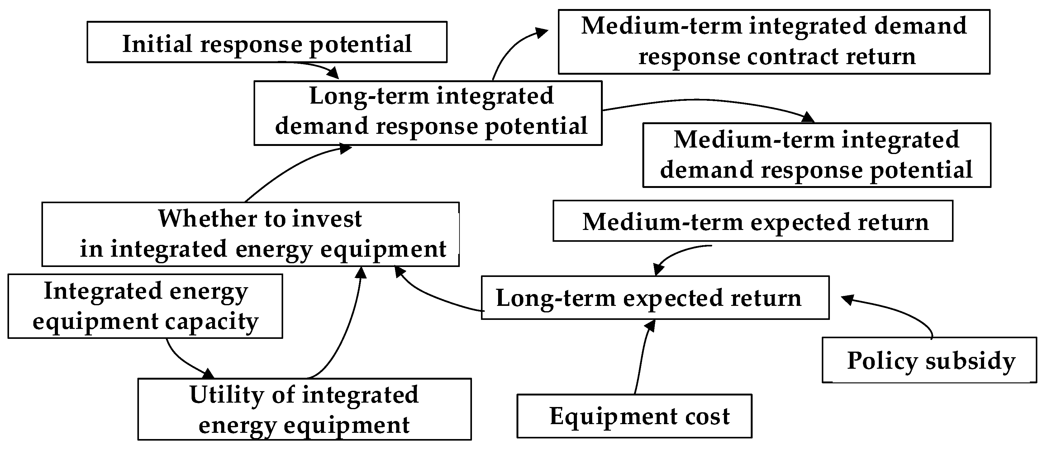
2.2.1. Long-Term Integrated Demand Response Decision Model

The user’s long-term integrated demand response decision, considers whether to replace high-efficiency integrated energy equipment, increase inventory or modify production lines, and other technological transformation projects that increase the potential of integrated demand response. The user’s long-term decision model considers the capacity of integrated energy equipment, equipment costs, and policy subsidy. Medium-term expected returns, long-term expected returns and other variables, among which policy subsidy as long-term incentives will have a greater impact on users’ decisions. Users comprehensively consider the effectiveness of integrated energy-use equipment and long-term expected returns, and make the long-term decision-making that whether to invest in integrated energy-use equipment. The specific stock flow diagram is shown in Figure 3, and the mathematical model is shown in formula.

$$S=\{\begin{array}{l}1,U_{\mathrm{ie}}>R_{le}\\ 0,other\end{array}$$

(1)

where S represents whether to invest in integrated energy equipment. U_ie represents integrated energy equipment utility. R_le represents long-term expected return.

$$U_{ie}=I_{el}$$

(2)

where I_el represents integration of integrated demand response income with equipment life.

$$R_{le}=R_{me}\times (1+R_{lu})+{\mathrm{P}}_s+{\mathrm{C}}_e$$

(3)

where R_me represents medium-term expected return. R_lu represents long-term user expectation improvement rate. P_s represents policy subsidy. C_e represents equipment cost.

$$P_{lr}=P_{ir}\times (1+R_{ai}\times S)$$

(4)

where P_lr represents long-term integrated demand response potential. P_ir represents initial response potential. R_ai represents response improvement rate after investing in integrated energy equipment.

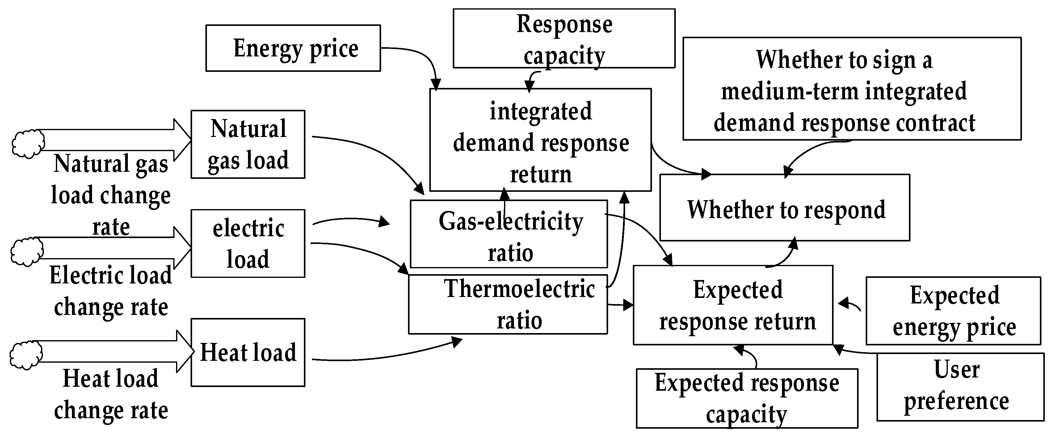
2.2.2. Medium-Term Integrated Demand Response Decision Model

The user’s medium-term decision considers whether to sign a medium-term integrated demand response contract. The user’s medium-term decision model considers variables such as contract duration, long-term integrated demand response potential, integrated demand response income, and expected response income, among which the long-term integrated demand response potential determines the medium-term integrated demand In response to the maximum capacity of the contract, the user comprehensively considers the medium-term integrated demand response contract revenue and medium-term expected revenue to make a medium-term decision on whether to sign an integrated demand response. The specific inventory flow chart is shown in Figure 4, and the mathematical model is shown in formula.

$$C_{mi}=\{\begin{array}{l}1,{\mathrm{R}}_{mc}>R_{me}\\ 0,other\end{array}$$

(5)

where, C_mi represents whether to sign a medium-term integrated demand response contract. R_mc represents medium-term integrated demand response contract revenue.

$$R_{mc}=P_{ic}+P_{lr}\times R_c$$

(6)

where, P_ic represents points for integrated demand response income over the duration of the contract. R_c represents revenue coefficient.

$$R_{me}=E_r\times (1+R_{mu})$$

(7)

where, E_r represents expected response revenue. R_mu represents long-term user expectation improvement rate.

$$P_{mr}=\{\begin{array}{l}{P}_{lr},C_{mu}\\ 0,other\end{array}$$

(8)

where, P_mr represents medium-term integrated demand response potential. C_mu represents user sign medium-term integrated demand response contracts.

2.2.3. Short-Term Integrated Demand Response Decision Model

The user’s integrated demand response decision model considers whether to participate in responding to IDR events on a daily scheduling time scale.

$$R=\{\begin{array}{l}1,C_{mu} \&\&R_{id}>E_r\\ 0,other\end{array}$$

(9)

where, R represents whether to respond. R_id represents integrated demand response revenue.

$$R_{si}=u(C_r,P_e),V_{sr}$$

(10)

where, R_si represents short-term integrated demand response revenue. C_r represents response capacity. P_e represents energy price. V_sr represents short-term integrated demand response simulation value.

$$R_{se}=u(C_{er},P_{ex},U_p)$$

(11)

where, R_se represents short-term expected response revenue. C_er represents expected response capacity P_ex represents expected energy price. U_p represents user preference.

The short-term integrated demand response decision model considers whether to sign a medium-term integrated demand response contract, the expected energy price, the user’s own preferences, the expected response capacity, the gas-electricity ratio and the thermoelectric ratio of the self-load, response capacity, energy prices and other variables. Among them, different users have different sensitivity to gas-electricity ratio and thermoelectricity ratio and users consider short-term integrated demand response income and expected response income to make a short-term decision on whether to respond. The specific inventory flow chart is shown in Figure 5, and the mathematical model is shown in formula.

3. Short-Term Integrated Demand Response Operation Simulation

The short-term integrated demand response operation simulation in the short-term integrated demand response decision model is a data source for the dynamic model of the integrated demand response system based on the medium- and long-term time dimension.

Based on the regional electric-pneumatic interconnected integrated energy system network, the coupling nodes connect the park-level heat network through combined cooling, heat and power (CCHP) to build a park-level cool-heat-electric-gas integrated energy system. Regional-level electricity-gas interconnection network is used as the input/output of CCHP in the park-level integrated energy system to provide a network architecture for connecting the park-level integrated energy system. Establish an integrated energy system and establish a scheduling model to obtain node energy prices and then use the energy network Node multi-energy load users are targeted, considering gas-electricity/thermal-electricity replaceable loads, establishing an integrated demand response model, simulating the short-term response capacity and short-term response benefits of users participating in integrated demand response, and passing them to users for response decisions. The simulated short-term integrated demand response income of the user is integrated according to the integrated demand response contract cycle and the integrated energy equipment usage cycle, and is used as an indicator for the user’s medium-term and long-term decisions. The linkage principle is shown in Figure 6.

3.1. Integrated Energy System Scheduling Model

The CCHP equipment of the coupling node in this paper mainly includes the use of combined heat and power, gas boilers, electric refrigerators, and absorption refrigerators. There are many related models [20,21], which are not repeated here. The electric-pneumatic network is connected to the park-level heating network to supply power and cooling while heating users. The structure of the integrated energy system is shown in Figure 7.

3.1.1. Heat Network Model

The main considerations are node flow balance, node power fusion, load taking characteristics, temperature constraints of water supply and return water, and heat transfer characteristics of the pipe section [22].

1. Node traffic balance

For any node in the heat network, the sum of the incoming hot water flow is equal to the sum of the outgoing flow, that is:

$${\displaystyle \sum _{j\in S_i^{pipe+}}{Q}_{j,t}^g}={\displaystyle \sum _{k\in S_i^{pipe-}}{Q}_{k,t}^g}$$

(12)

where, $S_i^{pipe+}$ and $S_i^{pipe-}$ is a set of pipes connected to node i and starting and ending from node i respectively; $Q_{j,t}^g$ is the mass flow of hot water in pipe j during period t.

2. Node temperature fusion

Hot water of different temperatures flows from different pipes to the same node and is mixed. After mixing, the hot water flowing into the different pipes from the same node has the same temperature, that is:

$${\displaystyle \sum _{j\in S_i^{pipe+}}{T}_{j,t}^O{Q}_{j,t}^g}=T_{k,t}^I{\displaystyle \sum _{k\in S_i^{pipe-}}{Q}_{k,t}^g}$$

(13)

where, $T_{j,t}^O$ is the hot water outlet temperature of pipe j in period t; $T_{k,t}^I$ is the temperature of the hot water in the pipeline k for period t.

3. Load taking characteristics

For a heat network branch that contains hot users, the load node i consumes heat at time t as the mass flow through the load node is water temperature reduced to return water temperature, which is:

$$h_{i,t}^L=c{Q}_{i,t}^g\left(T_{i,t}^g-T_{i,t}^h\right)$$

(14)

where, C is the specific heat capacity of hot water, taking 4.2 kJ/(kg·°C).

4. Variable supply and return water temperature constraints

In order to ensure the heat supply quality of heat sources and heat users, the supply and return water temperatures of heat sources and heat users need to be limited, that is:

$$T_{\min }^g\le T_{i,t}^g\le T_{\max }^g$$

(15)

$$T_{\min }^h\le T_{i,t}^h\le T_{\max }^h$$

(16)

5. Heat transfer characteristics of pipe sections

According to the modelling of heat transfer characteristics in [23], the steady-state heat transfer characteristics are as follows:

$$T_e=\left(T_a-T_s\right)\frac{x}{Rc\rho f}+T_s$$

(17)

where x is the distance between a point on the pipe section and the head of the pipe section; R is the thermal resistance per unit length of the pipe section; T s, T e, T a are the head end temperature of a pipe section, x is the temperature and outside temperature; f is the flow of hot water.

The transient heat transfer characteristics are as follows:

For places near the heat source, the transient process is short. After one adjustment and before the next adjustment, the temperature of the pipe section has reached a steady state. The transient heat transfer characteristics of the pipe section at these points can be expressed as:

$$T^i\left(x,t\right)=\{\begin{array}{l}\frac{\left(T_s^{i-1}-T_s^{i-2}\right)\left(1-\alpha x\right)}{\beta x}\left(t-t_{i-1}\right)\\ +\left(T_a-T_s^{i-2}\right)\alpha x+T_s^{i-2}t\in \left[t_{i-1},t_{i-1}+\beta x\right]\\ \left(T_a-T_s^{i-1}\right)\alpha x+T_s^{i-1}\hspace{1em}t\in \left(t_{i-1}+\beta x,t_i\right]\end{array}$$

(18)

where $T^i\left(x,t\right)$ is the temperature of the heat network pipe at time t from the heat source x during the i-th period; $T_s^{i-1}$ and $T_s^{i-2}$ are the temperature of the heat source at time t_i−1 and time t_i−2; i = 1,2,3, …

For places far away from the heat source, the steady state has not been reached during the adjustment process. The transient heat transfer characteristics of the pipe section at these points can be expressed as:

$$T^i\left(x,t\right)=\frac{\left(T_a-T_s^{i-1}\right)\alpha x+T_s^{i-1}-T^{i-1}\left(x,t_{i-1}\right)}{\beta x}\times \left(t-t_{i-1}\right)+T^{i-1}\left(x,t_{i-1}\right)\hspace{1em}t\in \left[t_{i-1},t_i\right]$$

(19)

where, $T^i\left(x,t\right)$ is the temperature of the heat network pipe at time t_i−1 from the heat source x during the i − 1 period; i = 1,2,3, …

3.1.2. Natural Gas Network Model

It mainly includes pipeline flow constraints, gas source point constraints, flow balance constraints, compressor constraints, and node pressure constraints [22].

1. Pipeline flow constraints

For an ideal adiabatic gas pipeline, considering the two-way flow of natural gas, the flow equation can be expressed as:

$${\tilde{Q}}_{ij,t}\left|{\tilde{Q}}_{ij,t}\right|=C_{ij}^2\left(p_{i,t}^2-p_{j,t}^2\right)$$

(20)

where, ${\tilde{Q}}_{ij,t}=(Q_{ij,t}^{in}+Q_{ij,t}^{out})/2$, which represents the average flow through pipe ij at time t, where $Q_{ij,t}^{in}$, $Q_{ij,t}^{out}$ are the first section of natural gas injection flow and the final natural gas output flow of pipeline ij at time t; C_ij is the constants related to the efficiency, temperature, length, inner diameter, and compression factor of pipeline ij; p_i,t, p_j,t, respectively the pressure value of the first and last nodes i and j at time t.

2. Natural gas source point constraint

$$Q_{n,\min }^N\le Q_{n,t}^N\le Q_{n,\max }^N$$

(21)

where, $Q_{n,\max }^N$, $Q_{n,\min }^N$, $Q_{n,t}^N$ are the upper and lower limits of the natural gas supply flow at the gas source point n and the output of the gas source at time t.

3. Traffic balance constraint

$$Q_{i,t}^N+{\displaystyle \sum _{i\in {\Omega }_j}{Q}_{ij,t}}+Q_{i,t}^{P2G}-Q_{i,t}^{G2P}-Q_{i,t}^L-Q_{i,t}^{CCHP}=0$$

(22)

where, $Q_{i,t}^N$ supply gas flow for node i at time t; $Q_{i,t}^{P2G}$ is the gas-to-electricity gas supply flow at node i at time t; $Q_{i,t}^{G2P}$ is the natural gas flow consumed by the gas turbine at node i at time t; $Q_{i,t}^L$ is the natural gas load at node i at time t. $Q_{i,t}^{CCHP}$ is the natural gas flow consumed by CCHP at node i at time t.

4. Compressor constraint

Using a simplified compressor model [24] is

$$p_{l,t}\le {\beta }_{com}{p}_{i,t}$$

(23)

where, β_com is the compression coefficient of the compressor, and p_l,t and p_i,t are the pressure values of nodes l and i.

5. Node pressure constraint

$$p_i^{\min }\le p_{i,t}\le p_i^{\max }$$

(24)

where, $p_i^{\max }$, $p_i^{\min }$ are the upper and lower limits of the pressure value at node i.

3.1.3. Grid Model

Node power balance, unit output constraints, climbing constraints, branch flow constraints, and electrical model gas and gas turbine related model constraints can be referred to in the literature [24,25], and will not be described here.

3.1.4. Objective Function

The park-level heat network is coupled to the regional-level electric-pneumatic interconnected integrated energy system network through CCHP equipment. The heat load is consumed by CCHP to supply electricity and natural gas. It only needs to consider the system’s dispatching costs for electricity and natural gas, mainly including the cost of thermal power generation, the cost of natural gas supply and the cost of electricity to gas, that is:

$$\min F={\displaystyle \sum _{t\in T}[{\displaystyle \sum _{g\in {\Omega }_G}{f}_1(P_{g,t}^G)}+{\displaystyle \sum _{n\in {\Omega }_N}{f}_2(Q_{n,t}^N)}}+{\displaystyle \sum _{l\in {\Omega }_{P2G}}{f}_3(P_{l,t}^{P2G})}]$$

(25)

where, F is the integrated operating cost of the system; T is the number of time sections; ${\Omega }_G$ is thermal power units; ${\Omega }_N$ is a set of natural gas source points; ${\Omega }_{G2P}$ is gas turbine unit; ${\Omega }_{p2G}$ is a unit for gas to electricity. $f_1\left(P_{g,t}^G\right)$ is the power generation cost function of thermal power unit g at time t, expressed as:

$$f_1\left(P_{g,t}^G\right)=a_g{\left(P_{g,t}^G\right)}^2+b_g{P}_{g,t}^G+c_g$$

(26)

where a_g, b_g, c_g are the parameters of the g consumption curve of the thermal power unit. $P_{g,t}^G$ is the active output of the thermal power unit g at time t.

$f_2\left(Q_{n,t}^N\right)$ is the cost function of gas supply point n at time t, which is expressed as:

$$f_2\left(Q_{n,t}^N\right)=C_{n,t}^N{Q}_{n,t}^N$$

(27)

where, $C_{n,t}^N$ is the gas supply cost coefficient of gas source point n at time t, $Q_{n,t}^N$ is the natural gas supply flow at gas source point n at time t.

$f_3\left(P_{l,t}^{P2G}\right)$ is the running cost function of electric gas l at time t, which is expressed as:

$$f_3\left(P_{l,t}^{P2G}\right)=C_{l,t}^{P2G}{P}_{l,t}^{P2G}$$

(28)

where, $C_{l,t}^{P2G}$ is the operating cost coefficient of electric gas l at time t, $P_{l,t}^{P2G}$ is the active power converted from electricity to gas l at time t.

3.2. Integrated Demand Response Model Considering Flexible Loads, Energy Storage, and Electric Vehicle as Participants

The multi-energy synergy of the integrated energy system expands the form of user participation in integrated demand response. Based on the difference in energy prices, users can choose different energy consumption methods to maximize their own energy efficiency. The main body is divided into flexible loads, energy storage and electric vehicles. In the power demand response, the response methods of flexible loads mainly include interruptible, translational, and transferable types, which are not described here, mainly considering the coupling and substitution relationship between multiple energy sources According to different ways of energy replacement, establish gas-electricity replacement load and heat-electricity replacement load model. For energy storage, in addition to considering traditional electric energy storage, you also need to establish models for gas storage systems and heat storage systems. For cars, the user’s electric vehicle driving characteristics are considered to establish a charge and discharge model for electric vehicles.

3.2.1. Node Energy Price

First, determine the node energy price according to the node energy balance constraints of the 3.1 integrated energy system scheduling model, as shown below:

$$P_{i,t}^G+P_{i,t}^W+P_{i,t}^{CCHP}+P_{i,t}^{G2P}-P_{i,t}^{P2G}-{\displaystyle \sum _{j\in {\Omega }_i}{P}_{ij,t}}=P_{i,t}^L$$

(29)

$$Q_{i,t}^N+{\displaystyle \sum _{i\in {\Omega }_j}{Q}_{ij,t}}+Q_{i,t}^{P2G}-Q_{i,t}^{G2P}-Q_{i,t}^{CCHP}=Q_{i,t}^L$$

(30)

The right side of the above formula is the node power load and the node natural gas load. $P_{i,t}^L$ increasing 1, the objective function value F (system operating cost) will correspondingly generate a marginal value corresponding to the power network node, and use this value to represent the node electricity price, which is recorded as:

$$p_{i,t}^e=\partial F/\partial P_{i,t}^L$$

(31)

Similarly, whenever the node natural gas load $Q_{i,t}^L$ increasing 1, the value of the objective function will also generate a marginal value corresponding to the natural gas network node. Use this value to represent the natural gas price of the node and record it as:

$$p_{i,t}^g=\partial F/\partial Q_{i,t}^L$$

(32)

3.2.2. Flexible Load Response Model

For user i, at time t, the electric load adjusted by the energy replacement project can be expressed as:

$$q_{i,t}^e=\overline{q_{i,t}^e}-L_{i,t}^{eg}-L_{i,t}^{eh}$$

(33)

The adjusted natural gas load is expressed as:

$$q_{i,t}^g=\overline{q_{i,t}^g}+{\rho }_{e/g}{L}_{i,t}^{eg}$$

(34)

The adjusted heat load is expressed as:

$$q_{i,t}^h=\overline{q_{i,t}^h}+{\rho }_{e/h}{L}_{i,t}^{eh}$$

(35)

where: $L_{i,t}^{eg}$ replace the electric load with gas for the user at time t; $L_{i,t}^{eh}$ replace the electric load with heat for the user at time t; $\overline{q_{i,t}^e}$ The user’s power load value before participating in the energy replacement project; $\overline{q_{i,t}^g}$ is the user’s natural gas load value before participating in the energy replacement project; $\overline{q_{i,t}^h}$ is the user’s heat load value before participating in the energy replacement project; ${\rho }_{e/g}$ is gas-electricity substitution coefficient; ${\rho }_{e/h}$ is the thermo-electric substitution factor.

3.2.3. Multi-Type Energy Storage Response Model

The electric energy storage system, gas storage system, and heat storage system can all participate in the integrated demand response, and the response can be achieved by switching the charging and discharging mode [26]. The dynamic mathematical model of electric energy storage is expressed as:

$$E_t^{ESS}=\left(1-{\mu }_e\right)E_{t-1}^{ESS}+\left(P_t^{ESS,in}{\eta }_{ech}-\frac{P_t^{ESS,dis}}{{\eta }_{edis}}\right)\times \Delta t$$

(36)

where $E_t^{ESS}$ is the storage capacity of electric energy storage during t period, μ_e is the loss rate of electric energy storage, $P_t^{ESS,in}$, $P_t^{ESS,dis}$ are the storage charge and discharge power during t period, and η_ech and η_edis represent the charge and discharge efficiency.

The mathematical model of gas storage dynamics is expressed as:

$$E_t^{GS}=\left(1-{\mu }_g\right)E_{t-1}^{GS}+\left(F_t^{GS,in}{\eta }_{gch}-\frac{F_t^{GS,dis}}{{\eta }_{gdis}}\right)\times \Delta t$$

(37)

where $E_t^{ESS}$ is the gas storage capacity of gas storage during t period, μ_g is the loss rate of gas storage, $F_t^{GS,in}$ and $F_t^{GS,dis}$ are the injection and extraction flow of the gas storage facility during the period t, and η_gch and η_gdis represent the injection and extraction efficiency.

The mathematical model of thermal storage dynamics is expressed as:

$$H_t^{HS}=\left(1-{\mu }_h\right)H_{t-1}^{HS}+\left(Q_t^{HS,in}{\eta }_{hch}-\frac{Q_t^{HS,dis}}{{\eta }_{hdis}}\right)\times \Delta t$$

(38)

where $H_t^{HS}$ is the heat storage capacity of thermal energy storage during t period, μ_h is the heat dissipation loss rate of heat storage, $Q_t^{HS,in}$, $Q_t^{HS,dis}$ are the heat storage and endothermic power during the period t, and η_hch and η_hdis represent the efficiency of heat absorption and heat release.

3.2.4. Electric Vehicle Response Model

Electric vehicle can be used as mobile energy storage to participate in integrated demand response, and the response is closely related to travel rules, mileage and atmospheric conditions such as sunlight. While achieving energy storage, it can meet users’ travel requirements. Frequent discharge of batteries will cause a certain amount of battery life for electric vehicles. In order to slow down the degradation of battery life, it is necessary to minimize the number of charge and discharge switching times [27] of the battery. It is assumed that the electric vehicle is only discharged once a day. The electric vehicle charge and discharge limit time t_lim can be expressed as:

$$t_{\lim }=\frac{P_d{t}_n+P_c{t}_l-\left(1-S_n\right)C_s}{P_c+P_d}$$

(39)

where, P_d, P_c, C_s are the charging and discharging power and rated capacity of the electric vehicle, t_n, t_l, and S_n are the current time and off-grid, respectively. Time and state of charge of the current time.

The state of charge when the electric vehicle leaves is satisfied by the following formula:

$$S_n\ge \frac{d_{next}\times W+Q_{\min }}{C_s}$$

(40)

where, d_next represents the next mileage of the electric vehicle, W is the power consumed per kilometer, and Q min is the minimum power of the electric vehicle.

Discharge capacity of electric vehicle $P_d^{EV}$. It can be expressed as:

$$P_d^{EV}=\frac{P_d}{P_c+P_d}\left[\left(t_l-t_n\right)P_c-\left(1-S_n\right)C_s\right]$$

(41)

Charging capacity of electric vehicle $P_c^{EV}$ can be expressed as:

$$P_c^{EV}=C_s\left(S_n+S_l-S_a-S_{\min }\right)$$

(42)

where, S_l, S_a, and S_min are the state of charge when offline, the state of charge when connected, and the lowest state of charge, respectively.

3.2.5. Objective Function

Based on microeconomics theory, users’ satisfaction with electricity, gas and heat is expressed as [28,29]:

$$v_{i,t}^e={\displaystyle {\int }_{q_{i,t}^{ne}}^{q_{i,t}^e}{\left(\frac{q}{a}\right)}^{\frac{1}{{\epsilon }_e}}dq}$$

(43)

$$v_{i,t}^g={\displaystyle {\int }_{q_{i,t}^{ng}}^{q_{i,t}^g}{\left(\frac{q}{a}\right)}^{\frac{1}{{\epsilon }_g}}dq}$$

(44)

$$v_{i,t}^h={\displaystyle {\int }_{q_{i,t}^{nh}}^{q_{i,t}^h}{\left(\frac{q}{a}\right)}^{\frac{1}{{\epsilon }_h}}dq}$$

(45)

where $v_i^e$, $v_i^g$ as well as $v_i^h$ Satisfaction of electricity, gas and heat for user i, $q_{i,t}^e$, $q_{i,t}^g$, $q_{i,t}^h$ For user i’s pure electrical load, pure gas load, pure thermal load, $q_{i,t}^{ne}$, $q_{i,t}^{ng}$, $q_{i,t}^{nh}$ represent the rigid load of electricity, natural gas, and heat, respectively of user i at time interval t; ε_e, ε_g, ε_h represent the user’s electricity, gas, and heat demand-price elasticity coefficient.

Maximizing node user utility is expressed as:

$$\max U_i={\displaystyle \sum _{t=1}^T\{{\lambda }_e\left[v_{i,t}^e(q_{i,t}^e)-q_{i,t}^e{p}_t^e\right]}+{\lambda }_g\left[v_{i,t}^g(q_{i,t}^g)-q_{i,t}^g{p}_t^g\right]+{\lambda }_h\left[v_{i,t}^h(q_{i,t}^h)-(q_{i,t}^{he}{p}_t^e+q_{i,t}^{hg}{p}_t^g)\right]\}$$

(46)

where U_i is the integrated energy efficiency of node user i, ${\lambda }_e$, ${\lambda }_g$ as well as ${\lambda }_h$. The weight coefficients for user electricity, gas and heat use, $q_{i,t}^{he}$, $q_{i,t}^{hg}$ are electric energy and natural gas consumed by CCHP for pure thermal load, $p_t^e$, $p_t^g$ are the node electricity price and the node gas price obtained from the integrated energy system scheduling model. Finally, the short-term response income is classified according to the proportion of electricity, gas, and heat load. According to the short-term response income and short-term response corresponding to different gas-to-electricity ratios and thermoelectric ratios, expected returns make short-term response decisions [30,31,32].

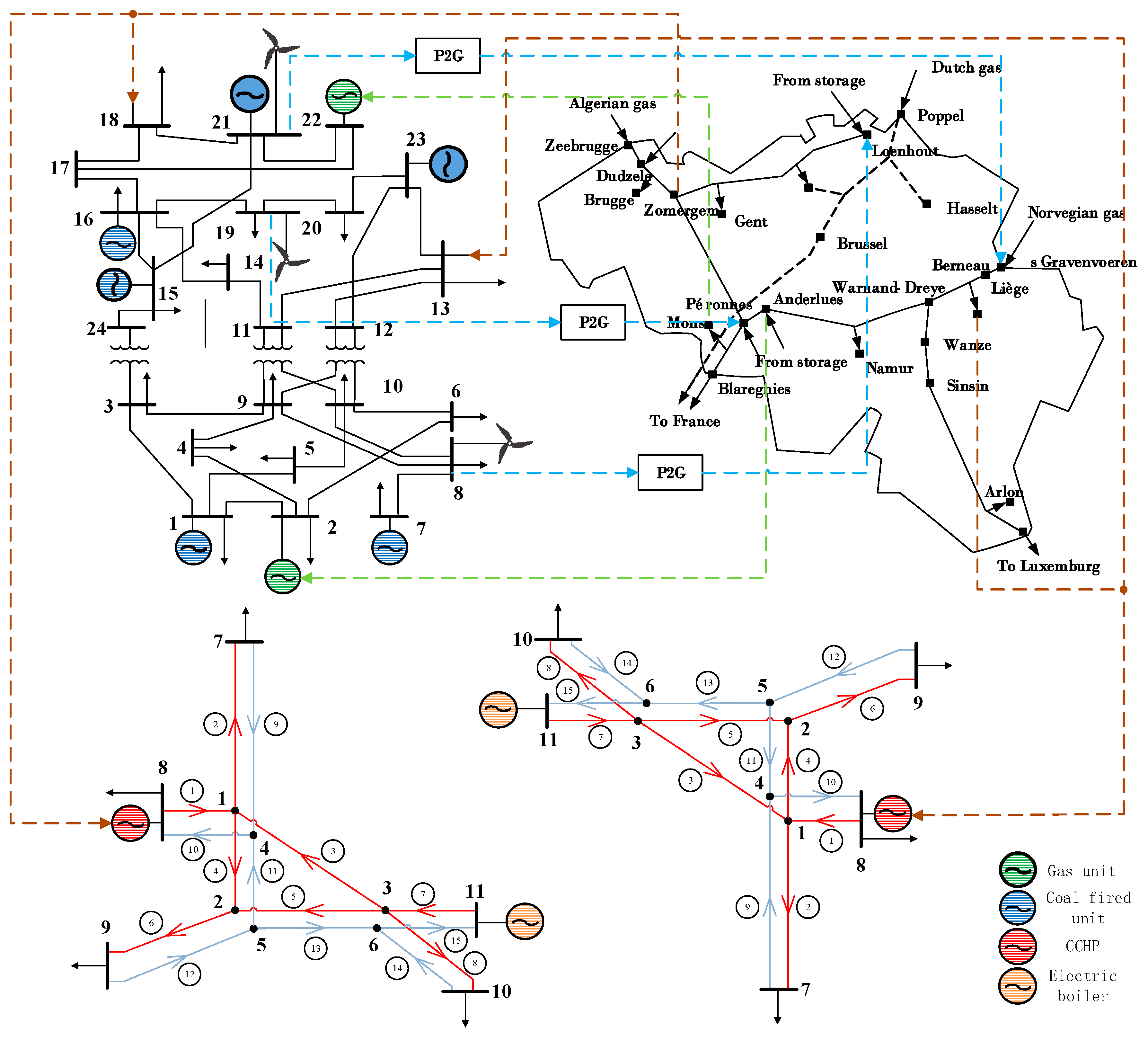
4. Analysis of Examples

4.1. Study Data

In the underlying integrated energy system dispatching network, the improved IEEE24-node power grid and the Belgian 20-node gas network are coupled by electricity-to-gas, gas turbines and other equipment to form an upper-layer electric-pneumatic interconnected network. The improved campus-level heat network will pass CCHP according to [17]. It is connected to the electricity-gas network to form a park-level cool-heat-electricity-gas integrated energy system as shown in Figure 8, where, the IEEE24 node system has eight generating units; nodes 2 and 22 are gas turbines, which are respectively connected to the natural gas network. Anderlues is connected to the Mons node; nodes 13 and 18 are combined cooling and heating power units, which are connected to the Liege and Zomergem nodes of the natural gas network, eight nodes of the thermal network I and eight nodes of the thermal network II; power nodes 8, 19 and 21 each connected to a wind power unit with a rated output of 100 MW. In order to maximize the wind power and avoid the natural gas network line blockage, the input end of the electricity to gas is also connected to nodes 8, 19 and 21 of the power network, and the output end is connected to the Loenhout, Peronnes, and Voeren nodes in the natural gas network are connected. The 20-node natural gas system in Belgium includes 21 gas pipelines, two pressurized stations, and two gas source points W1 and W2. The heating networks I and II are connected to an electric boiler at 11 nodes, respectively. The upper and lower limits of output are 300 MW and 40 MW, and the efficiency is 0.95.

4.1.1. Equipment Related Parameters

The relevant parameters of the gas turbine are shown in

Table 1. Gas turbine related parameters.

Unit	Power Network Node	Natural Gas Network Node	Active Upper Limit (MW)	Active Lower Limit (MW)	Conversion Efficiency (%)
GT1	2	Anderlues	104	0	43%
GT2	18	Liege	80	0	43%
GT3	22	Mons	80	0	43%

. The relevant parameters of the electric-to-gas conversion are shown in

Table 2. P2G related parameters.

Unit	Power Network Node	Natural Gas Network Node	Enter Upper Limit (MW)	Enter Lower Limit (MW)	Methane Conversion Efficiency (%)	Run Cost ($/MW)
P2G1	8	Loenhout	88	0	60%	1.5
P2G2	19	Peronnes	88	0	60%	1.6
P2G3	21	Voeren	66	0	60%	1.5

. The CCHP on the heating network I and the heating network II have the same configuration parameters, as shown in

Table 3. CCHP related parameters.

Name	Maximum Output (MW)	Lower Output Limit (MW)	Effectiveness (%)
Electric refrigerator	200	0	4
Absorption refrigeration	200	0	1.1
Cogeneration	350	0	0.75
Gas boiler	500	0	0.9
Heat Exchanger	10,000	0	0.9

. On this basis, take coupling node 13 and coupling node 18 in the power grid for comparison and analysis. It is assumed that the two nodes have the same load before the response, corresponding to user 1 and user 2, respectively. And their energy consumption preferences and expected response benefits to the integrated demand response are different.

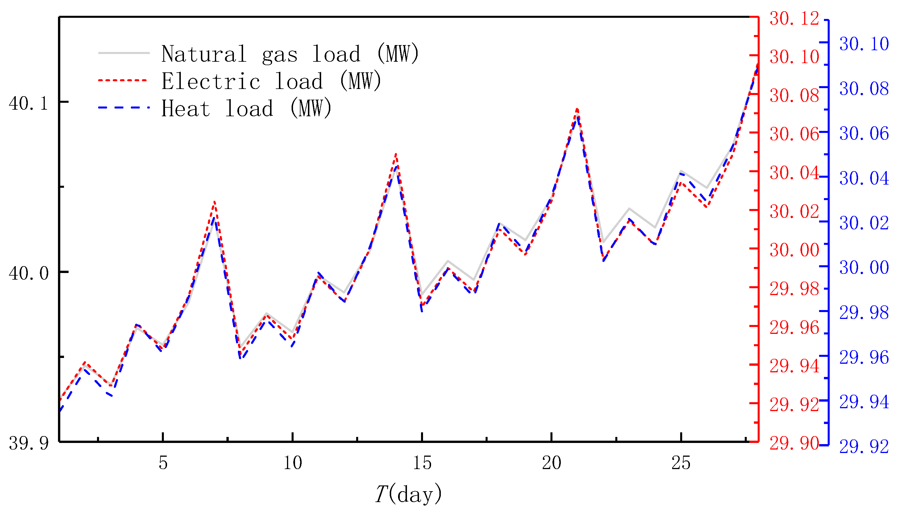
4.1.2. Flexible Load Data

Take the load of four weeks in a month in the second year of winter to analyze the response of flexible load users to the integrated demand response project. The growth of gas load, heat load, and electrical load over time in one month is shown in Figure 9. The growth from Monday to Friday was relatively stable, and the load increased significantly every weekend.

4.1.3. Energy Storage Load Data

Take the load of four quarters in a year to analyze the participation of energy storage users in integrated demand response projects. The change of electricity, gas and heat load over time in a year is shown in Figure 10.

4.1.4. Changes in Mileage of Electric Vehicle

The daily response of electric vehicle users is affected by the satisfaction of the mileage and the response income. The daily mileage is approximately log-normally distributed. The random distribution of the mileage of the user 1 within a month and the responses are shown in Figure 11.

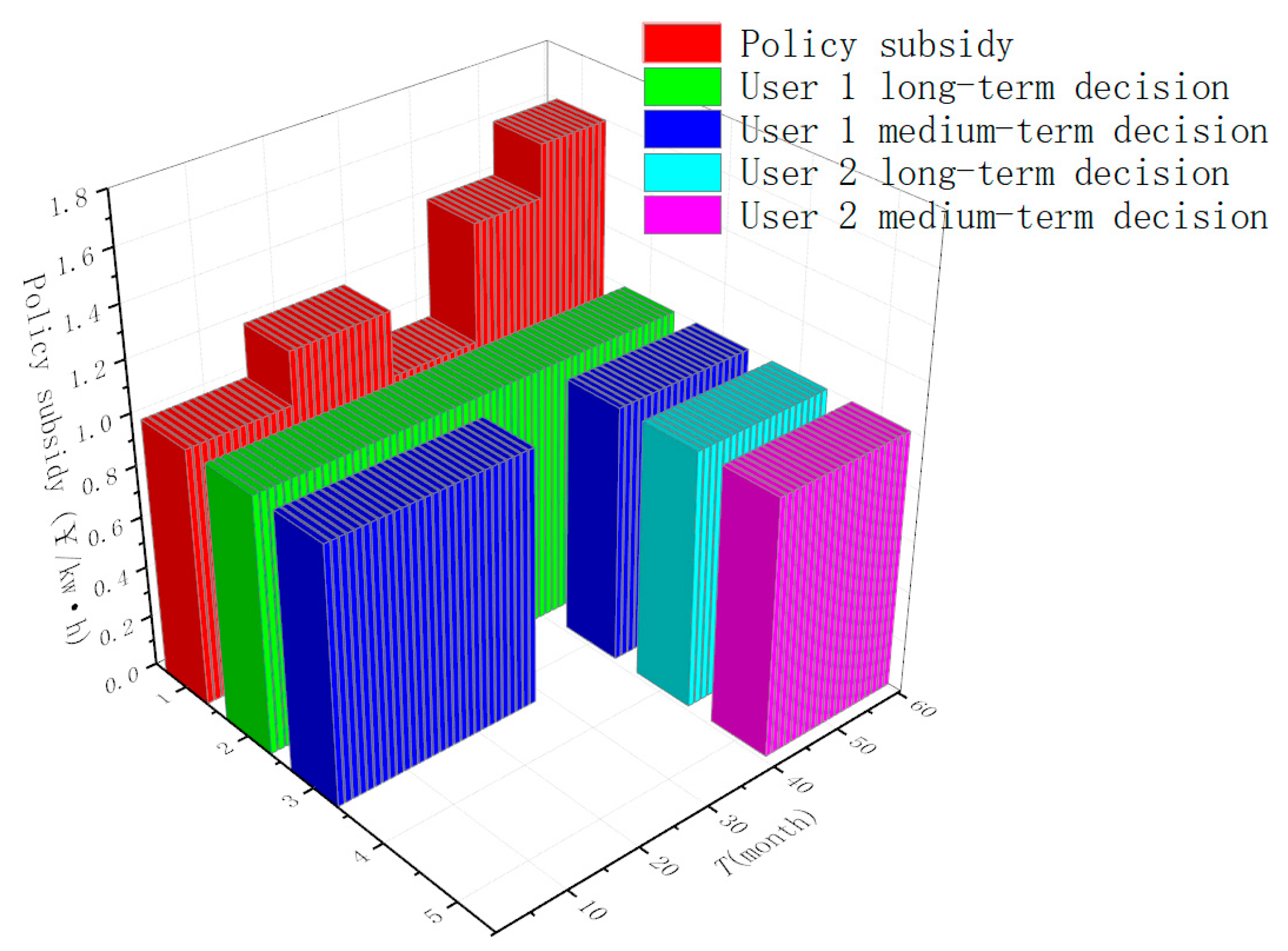
4.1.5. Changes in Policy Subsidy

Assume that the integrated demand response project has been implemented for five years, and the policy subsidy reflects the long-term incentive level. In order to compare and analyze the impact of different long-term incentive levels on the medium- and long-term integrated demand response decision, it is assumed that the policy subsidy changes are shown in Figure 12.

In the second year, the policy subsidy increased compared to the first year, but in the third year, the policy subsidy fell to a trough due to some reasons, and in the fourth and fifth years, it returned to the high subsidy level.

4.1.6. Changes in Policy Subsidy

According to the short-term integrated demand response operation simulation, the short-term expected response benefits are shown in

Table 4. Short-term expected response income.

Gas-Electricity Ratio	Thermoelectric Ratio	Short-Term Expected Response Returns ($)
Greater than 1.1875 and Less than 1.33	Greater than 0.9375 and less than 1	26,931.453
Greater than 1.1875 and Less than 1.33	Greater than 1	25,435.261
Greater than 1.1875 and Less than 1.33	Less than 0.9375	25,435.261
Greater than 1.33	/	26,931.453
Less than 1.1875	/	17,954.302

, and the different parameters of different types of users’ response to the long-term integrated demand are shown in

Table 5. Differential parameters for medium- and long-term response.

User	Medium-Term Yield Improvement	Long-Term Yield Improvement Rate	Equipment Cost ($)
Flexible load user 1	9	0.15	835
Flexible load user 2	9	0.2	835
Energy storage user 1	9	0.15	17,167
Energy storage user 2	9	0.2	17,167
Electric vehicle users1	9	0.15	33,335
Electric vehicle users 2	9	0.2	33,335

.

4.2. Analysis of Short-Term Integrated Demand Response Simulation Results

Due to the continuous use characteristics of the energy storage equipment, the investment period of the energy storage equipment is set to half a year, and the investment equipment will be used. Therefore, the long-term energy storage equipment investment decision is not considered to analyze the short-term response benefits of energy storage users. It mainly analyzes the short-term response of flexible loads and electric vehicle users. The short-term response income simulation results are shown in

Table 6. Short-term response benefit simulation results.

Gas-Electricity Ratio	Thermoelectric Ratio	Short-Term Response Income ($)
Greater than 1.1875 and Less than 1.33	Greater than 0.9375 and less than 1	28,427.645
Greater than 1.1875 and Less than 1.33	Greater than 1	26,931.453
Greater than 1.1875 and Less than 1.33	Less than 0.9375	26,931.453
Greater than 1.33	/	25,435.261
Less than 1.1875	/	13,465.727

.

4.2.1. Analysis of Short-Term Response of Flexible Load Users

For flexible loads, the response situation is more closely related to time. The changes in weekday and holiday loads make users’ changes in expected response revenue more obvious. Therefore, this article analyzes the response of flexible load users to participate in integrated demand response from weekly load changes. The response within four weeks is shown in Figure 13. Among them, “1” on the ordinate represents the user’s participation in the response, and the abscissa is the number of days. In the four weeks shown in Figure 12, users have higher responsiveness from Monday to Friday and relatively few weekends. The main reason is that users have higher requirements for energy consumption on weekends and higher expected returns on integrated demand response projects, so they have fewer response times.

4.2.2. Analysis of Short-Term Response of Electric Vehicle Users

The response of the electric vehicle is shown in Figure 14. In conjunction with Figure 11 and Figure 14, when the electric vehicle’s mileage did not exceed 58 km, the user chose to respond. This is mainly because when the mileage did not exceed 58 km, the user’s travel satisfaction was within the acceptable range. However, when the mileage exceeded 58 km, the response was not enough to make up for the user’s request for travel satisfaction, and it did not respond.

4.3. Long-Term Integrated Demand Response Analysis of Flexible Loads, Energy Storage, and Electric Vehicle

4.3.1. Analysis of Medium- and Long-Term Decisions for Flexible Load Users

Vensim software was used to simulate the long-term integrated demand response project. The medium- and long-term integrated demand response situation of flexible load users is shown in Figure 15, where the red block is the subsidy level, and the long-term decision of users 1 and 2 is 1 for integrated investment. Energy equipment, when it was 0, did not invest. When the medium-term decision was 1, it means that it signed a medium-term integrated demand response contract, and when it was 0, it means that it did not sign a contract. User 1 started to invest in integrated energy-use equipment after the second year subsidy policy was raised, and A medium-term integrated demand response contract was signed, but its sensitivity to policy subsidy was not high, and even if the subsidy slightly declined in the third year, its investment decision on integrated energy-using equipment was unchanged, and an integrated demand response contract was also signed. User 2 first began to invest in integrated energy equipment in 2015, actively participated in integrated demand response projects and signed medium-term integrated demand response contracts, but its sensitivity to policy subsidy was high. When the subsidy fell in the third year, it was decided not to invest in integrated energy equipment. However, a medium-term contract is still signed to ensure integrated demand response participation.

4.3.2. Medium- and Long-Term Decision Analysis of Energy Storage

The response of energy storage is greatly related to seasonal changes, and the changes in winter and summer make the response gains of energy storage significantly different, so this section analyzes the medium-to-long-term decisions of energy storage users from the changes in seasonal load. According to Figure 10 quarterly load changes of energy storage users, and the medium-to-long-term integrated demand response of energy storage users including electricity storage, gas storage, and heat storage systems are shown in Figure 16.

Combining Figure 12 and Figure 16, User 1 had a higher preference for the energy consumption of electric loads, and has been investing in electric energy storage equipment since the first year, but did not invest in heat and gas storage in the season when the heat load and gas load were small. Equipment, after the policy subsidy rose sharply in the later period, began to invest in energy storage equipment regardless of the season. User 2’s preference for electricity, heat, and gas was relatively balanced, and in the first year of policy subsidy levels, no energy storage equipment was invested. After the subsidy rose in the second year, it has been investing in energy storage equipment and responded positively.

4.3.3. Analysis of Medium- and Long-Term Integrated Decision of Electric Vehicle

According to Table 5, it can be seen that the long-term profit improvement rate of electric vehicle user 2 is higher than that of user 1, which reflects that user 2’s travel satisfaction is higher than that of user 1. The medium-to-long-term integrated demand response of electric vehicle users is shown in Figure 17.

Faced with the first year of policy subsidy, users with low travel satisfaction 1 began to invest in electric vehicles. Until the third year, subsidies fell, and the upgrading of electric vehicles was stopped, but investment was resumed after the subsidy rose. The travel satisfaction of 2 was high. In the face of the first to third year of subsidy, they were reluctant to invest in electric vehicles. After the sharp increase in the fourth year, they began to invest in electric vehicles.

5. Conclusions

Based on system dynamics, this paper analyzes the long-term, medium-term, and short-term integrated demand response behavior of demand response resources in different time dimensions, and establishes an integrated demand response model based on the long-term time dimension. Considering flexible loads, energy storage, and electric vehicles as IDR participation, the main body, established an integrated energy system scheduling and integrated demand response model, simulates the benefits of user participation in IDR, and provides a data source for the long-term integrated demand response model. The example is based on long-term incentives based on policy subsidy, and compares and analyzes different long-term incentive levels and regions: location, user energy preferences, and other characteristics of flexible load, energy storage, and electric vehicle users’ response behavior in different time dimensions. When users of different types and locations face incentive signals from policy subsidy, their response decisions are significantly different. In the future, the uncertain impact of user response can be considered, and the user energy consumption behavior will continue to be deepened. We will analyze the multiple behaviors of different users, and do further research on a good source-charge interaction mechanism, considering issues such as economics, environmental protection, voltage quality and safety.

References

1. National Guiding Opinions on Promoting the Development of “Internet +” Smart Energy [EB/OL]. Available online: http://rench.smesdgov.cn/ecdomain/jnrc/index/gmbgegiiejafbbodjlocigkedbdjccbo/20160308130440106.html (accessed on 8 March 2016).
2. Wang, W.; Wang, D.; Jia, H.; Chen, Z.; Guo, B.; Zhou, H.; Fan, M. Review of steady-state analysis of typical regional integrated energy system under the background of energy internet. Proc. CSEE 2016, 36, 3292–3305. (In Chinese) [Google Scholar]
3. Wang, W.; Wang, D.; Jia, H.; Chen, Z.; Guo, B.Q.; Zhou, H.M.; Fang, M.W. Steady state analysis of electricity-gas regional integrated energy system with consideration of NGS network status. Proc. CSEE 2017, 37, 1293–1304. (In Chinese) [Google Scholar]
4. Sun, H.; Guo, Q.; Pan, Z. Energy Internet: Ideas, Architecture and Future Perspectives. Autom. Electr. Power Syst. 2015, 39, 1–8. (In Chinese) [Google Scholar]
5. Sun, H.; Pan, Z.; Guo, Q. Research on Integrated Energy and Energy Management: Challenges and Prospects. Autom. Electr. Power Syst. 2016, 40, 1–8. [Google Scholar]
6. Tafreshi, S.M.M.; Lahiji, A.S. Long-term market equilibrium in smart grid paradigm with introducing demand response provider in competition. IEEE Trans. Smart Grid 2015, 6, 2794–2806. [Google Scholar] [CrossRef]
7. Favre-Perrod, P. A vision of future energy networks. In Proceedings of the 2005 IEEE Power Engineering Society Inaugural Conference and Exposition in Africa, Durban, South Africa, 11–15 July 2005; pp. 13–17. [Google Scholar]
8. Geidl, M.; Koeppel, G.; Favre-Perrod, P.; Klockl, B.; Andersson, G.; Frohlich, K. Energy hubs for the future. Power Energy Mag. IEEE 2006, 5, 24–30. [Google Scholar] [CrossRef]
9. Wu, J. Drive and Status Quo of the Development of European Integrated Energy System. Autom. Electr. Power Syst. 2016, 40, 1–7. (In Chinese) [Google Scholar]
10. Bozchalui, M.C.; Hashmi, S.A.; Hassen, H.; Canizares, C.A.; Bhattacharya, K. Optimal operation of residential energy hubs in smart grids. IEEE Trans. Smart Grid 2012, 3, 1755–1766. [Google Scholar] [CrossRef]
11. Lund, H.; Andersen, A.N. Optimal designs of small CHP plants in a market with fluctuating electricity prices. Energy Convers. Manag. 2005, 46, 893–904. [Google Scholar] [CrossRef]
12. Fragaki, A.; Andersen, A.N. Conditions for aggregation of CHP plants in the UK electricity market and exploration of plant size. Appl. Energy 2011, 88, 30–40. [Google Scholar] [CrossRef]
13. Fragaki, A.; Andersen, A.N.; Toke, D. Exploration of economical sizing of gas engine and thermal store for combined heat and power plants in the UK. Energy 2008, 33, 59–70. [Google Scholar] [CrossRef]
14. Buber, T.; von Roon, S.; Gruber, A.; Conrad, J. Demand response potential of electrical heat pumps and electric storage heaters. In Proceedings of the IECON 2013-39th Annual Conference of the IEEE Industrial Electronics Society, Vienna, Austria, 10–13 November 2013; pp. 8028–8032. [Google Scholar]
15. Gao, Y.; Wang, P.; Xue, Y. Collaborative planning of integrated electricity-gas energy systems considering demand side management. Autom. Electr. Power Syst. 2018, 42, 3–11. (In Chinese) [Google Scholar]
16. Brahman, F.; Honarmand, M.; Jadid, S. Optimal electrical and thermal energy management of a residential energy hub, integrating demand response and energy storage system. Energy Build. 2015, 90, 65–75. [Google Scholar] [CrossRef]
17. Bradley, P.; Leach, M.; Torriti, J. A review of the costs and benefits of demand response for electricity in the UK. Energy Policy 2013, 52, 312–327. [Google Scholar] [CrossRef] [Green Version]
18. Ruan, W.; Wang, B.; Li, Y.; Yang, S. Customer response behavior in time-of-use price. Power Syst. Technol. 2012, 36, 86–93. (In Chinese) [Google Scholar]
19. Wang, B.; Yang, X.; Yang, S. System Dynamics Analysis of Demand Response Potential and Effects Based on Medium- and Long Term Time Dimensions. Chin. J. Electr. Eng. 2015, 35, 6368–6377. (In Chinese) [Google Scholar]
20. Wang, J.; Gu, W.; Lu, S.; Zhang, C.; Wang, Z.; Tang, Y. Collaborative planning of multi-region integrated energy system combined with heat network model. Autom. Electr. Power Syst. 2016, 40, 17–24. (In Chinese) [Google Scholar]
21. Wang, C.S.; Hong, B.W.; Guo, L.; Zhang, D.J.; Liu, W.J. A general modeling method for optimal dispatching of combined cooling, heating and power microgrid. Proc. CSEE 2013, 33, 26–33. (In Chinese) [Google Scholar]
22. Dong, S.; Wang, C.; Xu, S.; Zhang, L.; Zha, H.; Liang, J. Day-ahead optimal scheduling of electricity-gas-heat integrated energy system considering dynamic characteristics of network. Autom. Electr. Power Syst. 2018, 42, 12–19. (In Chinese) [Google Scholar]
23. Yao, S.; Gu, W.; Zhang, X. Effect of Heating Network Characteristics on Ultra-short-term Scheduling of Integrated Energy System. Autom. Electr. Power Syst. 2018, 42, 89–90. (In Chinese) [Google Scholar]
24. Wei, Z.; Zhang, S.; Sun, G.; Zang, H.; Chen, S.; Chen, S. Power-to-gas considered peak load shifting research for integrated electricity and natural-gas energy systems. Proc. CSEE 2017, 37, 4601–4609. (In Chinese) [Google Scholar]
25. Correa-Posada, C.M.; Sanchez-Martin, P. Integrated power and natural gas model for energy adequacy in short-term operation. IEEE Trans. Power Syst. 2015, 30, 3347–3355. [Google Scholar] [CrossRef]
26. Yang, X.; Zhang, Y.; Lu, J.; Zhao, B.; Huang, F.T.; Qi, J.; Pan, H.W. Blockchain-based automated demand response method for energy storage system in an energy local network. Proc. SCEE 2017, 37, 3703–3716. [Google Scholar]
27. Li, Z.; Zhao, S.; Liu, Y. Control strategy and application of distributed electric vehicle energy storage. Power Syst. Technol. 2016, 40, 442–450. [Google Scholar]
28. Ren, Y.; Zhou, M.; Li, G. Bi-level model of electricity procurement and sale strategies for electricity retailers considering users’ demand response. Autom. Electr. Power Syst. 2017, 41, 30–36. (In Chinese) [Google Scholar]
29. Thimmapuram, P.R.; Kim, J. Consumers’ price elasticity of demand modeling with economic effects onelectricity markets using an agent-based model. IEEE Trans. Smart Grid 2013, 4, 90–397. [Google Scholar] [CrossRef]
30. Song, X.; Lin, H.; De, G.; Li, H.; Fu, X.; Tan, Z. An Energy Optimal Dispatching Model of an Integrated Energy System Based on Uncertain Bilevel Programming. Energies 2020, 13, 477. [Google Scholar] [CrossRef] [Green Version]
31. Liu, Z.; Yu, H.; Liu, R.; Wang, M.; Li, C. Configuration Optimization Model for Data-Center-Park-Integrated Energy Systems Under Economic, Reliability, and Environmental Considerations. Energies 2020, 13, 448. [Google Scholar] [CrossRef] [Green Version]
32. Lv, Z.; Wu, Z.; Dou, X.; Zhou, M.; Hu, W. Distributed Economic Dispatch Scheme for Droop-Based Autonomous DC Microgrid. Energies 2020, 13, 404. [Google Scholar] [CrossRef] [Green Version]
Figure 1. Medium- and long-term integrated demand response modeling process for integrated energy systems.
Energies 13 00710 g001
Figure 2. Causal loop diagram.
Energies 13 00710 g002
Figure 3. Long-term integrated demand response decision module stock flow chart.
Energies 13 00710 g003
Figure 4. Medium-term integrated demand response decision module stock flow chart.
Energies 13 00710 g004
Figure 5. Short-term integrated demand response simulation module stock flow chart.
Energies 13 00710 g005
Figure 6. Modeling schematic.
Energies 13 00710 g006
Figure 7. Integrated energy system structure.
Energies 13 00710 g007
Figure 8. Integrated energy system example diagram of combined power grid, gas network and heat network.
Energies 13 00710 g008
Figure 9. Flexible load growth in a month.
Energies 13 00710 g009
Figure 10. Quarterly load change.
Energies 13 00710 g010
Figure 11. Electric vehicle mileage.
Energies 13 00710 g011
Figure 12. Policy subsidy change.
Energies 13 00710 g012
Figure 13. Short-term response of flexible load users.
Energies 13 00710 g013
Figure 14. Short-term response of electric vehicle users.
Energies 13 00710 g014
Figure 15. Medium- and long-term decision-making of flexible load users.
Energies 13 00710 g015
Figure 16. Long-term decision-making of energy storage users.
Energies 13 00710 g016
Figure 17. Medium- and long-term decision-making of electric vehicle.
Energies 13 00710 g017