Article

Demand Response Model Development for Smart Households Using Time of Use Tariffs and Optimal Control—The Isle of Wight Energy Autonomous Community Case Study

1
School of Energy and Electronic Engineering, University of Portsmouth, Portsmouth PO1 3DJ, UK
2
School of Engineering, Newcastle University, Newcastle upon Tyne NE17RU, UK
3
School of Mathematics and Physics, University of Portsmouth, Portsmouth PO1 2UP, UK
4
Faculty of Technology, University of Portsmouth, Portsmouth PO1 3AH, UK
5
Isle of Wight Council, County Hall, Newport, Isle of Wight PO30 1UD, UK
*
Authors to whom correspondence should be addressed.
Energies 2020, 13(3), 541; https://doi.org/10.3390/en13030541
Submission received: 20 December 2019 / Revised: 19 January 2020 / Accepted: 21 January 2020 / Published: 22 January 2020
(This article belongs to the Special Issue Optimal Control and Nonlinear Dynamics in Electrical Power Systems)

Abstract

:
Residential variable energy price schemes can be made more effective with the use of a demand response (DR) strategy along with smart appliances. Using DR, the electricity bill of participating customers/households can be minimised, while pursuing other aims such as demand-shifting and maximising consumption of locally generated renewable-electricity. In this article, a two-stage optimization method is used to implement a price-based implicit DR scheme. The model considers a range of novel smart devices/technologies/schemes, connected to smart-meters and a local DR-Controller. A case study with various decarbonisation scenarios is used to analyse the effects of deploying the proposed DR-scheme in households located in the west area of the Isle of Wight (Southern United Kingdom). There are approximately 15,000 households, of which 3000 are not connected to the gas-network. Using a distribution network model along with a load flow software-tool, the secondary voltages and apparent-power through transformers at the relevant substations are computed. The results show that in summer, participating households could export up to 6.4 MW of power, which is 10% of installed large-scale photovoltaics (PV) capacity on the island. Average carbon dioxide equivalent (CO2e) reductions of 7.1 ktons/annum and a reduction in combined energy/transport fuel-bills of 60%/annum could be achieved by participating households.

Graphical Abstract

1. Introduction

To reduce the load on the grid during peak-demand periods or to maximise the use of clean energy, variable energy price schemes have been suggested [1,2,3]. These schemes can provide a reduced cost of electricity during off peak consumption, or when surplus energy is being generated that would otherwise be lost [2]. Variable pricing can be more effective with the use of demand response (DR) strategy along with smart appliances. DR is a scheme that enables changes in the electricity usage by end-use customers in response to signals from the electricity supplier, or changes in the price of electricity over time [4]. DR enables shifts in demand patterns that can be useful for the operation of the power grid [5]. Peak demand can be reduced and shifted to off peak periods or matched to the pattern of local generation. Using DR, the electricity bill of participating customers can be reduced and they can benefit from other incentives offered by the supplier [6]. It is clear that the home energy management sector is evolving at a fast rate, with a growing number of ‘smart’ energy devices—including for instance smart home heating controls, smart lighting and appliance controls, energy generation devices such as photovoltaics (PV) panels, and smart residential battery storage products—now becoming available on the market [7,8]. DR has the potential to promote multiple benefits across all stakeholders. A reduction in energy cost to the customer could be created, with a revenue generation for prosumers. An increase could be achieved in localised generation capacity for the supplier, with a reduced distribution reinforcement cost for the distribution network operator (DNO). Combined, energy savings can result in a reduction in greenhouse gas (GHG) emissions. Reducing GHG emissions is essential if the UK is to meet its Paris agreement obligations and the Government’s “Net Zero” target [9]. The UK government has produced a recent report which raises these points [10]. The same report indicates that there are risks as well in terms of the potential for energy rebound effects (an unintended increase in demand at certain periods), vulnerability to changes in energy pricing, and data security implications. Moreover, there may be potential barriers to the deployment of home energy controls, and new challenges for other stakeholders in the energy ecosystem, such as DNOs, and energy suppliers and generators. A number of barriers to the uptake of home energy controllers, or to the realisation of their possible benefits, have been identified [10]. These barriers can be categorised as follows: (i) technical barriers, (ii) interoperability of equipment and standardization, (iii) security and privacy concerns, (iv) economic considerations, (v) regulatory and market barriers, (vi) consumer behaviour and awareness, and (vii) barriers related to the smart meter rollout. The technical and practical feasibility of DR as a consequence of these barriers have yet to be proven beyond the household and small community scale, particularly within the UK whereby energy distribution is owned by a government-regulated monopoly. We believe that the implementation of the proposed DR scheme is technically feasible using elements that already exist in the market, such as smart metering infrastructures, Time of use tariffs (which are currently offered by some UK energy suppliers), smart devices with communication capabilities along with a small networked computer in each household which will take the role of DR controller. There is, for example, a standardised communications data model for automated DR known as OpenADR [11], as well as commercial software and hardware components for industrial DR applications that use it. Such hardware components already include an automated DR controller that sits at the industrial customer’s premises. Moreover, the emergence of networked automation tools, such as the free web-based automation protocol If-This-Then-That (IFTTT) [12], and their adoption by smart appliance manufacturers, will facilitate the implementation of residential DR schemes, such as the one modelled in this article.
To implement the DR scheme, there is a need of transformation of the current state of the distribution system towards a smart grid environment/smart energy community for which Ghiani et al. [13] have presented the required planning actions. In their study, a pathway has been presented towards increasing the localised renewable energy generation matched to the consumption utilising combinations of various technologies, including energy storage, photovoltaics, smart grid communications, and appropriate IT infrastructure. The specific smart grid architecture under which the proposed demand response scheme will operate has not been fully defined yet. However, we envisage that it will have elements in common with the architecture described in [14], where a smart grid architecture model (SGAM) methodology is used to define the architecture that will support a local energy market operating in a residential microgrid, which utilises a block-chain based information system.
For the households, the application of DR strategies has been investigated by researchers to schedule the operation of: space heating systems [15], electric water heating systems [16], heat pumps [17], photovoltaics-battery systems [18], wind energy generation [19], solar hot water systems [20], washing machines, and dishwashers [21]. Various approaches have been used for modelling such as the Markovian model [22], game theory [23], the home energy management system (HEMS) model [24], mixed integer linear programing [25] and the ant colony optimisation algorithm [26]. However, at present, there are no DR models that incorporate all the commercially available DR functions, combined with the ability to differentiate property size/use on a community-sized area.
In this work, a price-based implicit [27] DR methodology is described for the application of complete households incorporating key DR features, such as an electric vehicle (EV) as a potential-detachable battery bank, the ability to export electricity to generate revenue, and the incorporation of Time of use (TOU) tariffs, in addition to rooftop PV power generation, smart residential battery storage, electric storage heater, electric water heater, a smart meter, and a DR controller. The local DR tasks will be executed by DR controllers located at customer’s premises, which will receive TOU information from the energy supplier and will interact with the local smart devices (e.g., immersion heaters, etc.). It is envisaged that the proposed DR scheme will be part of a local energy market, which will determine the values of the time of use tariffs on a daily basis. The composition, operation, and financing of the local energy market will be the subject of future work.
A case study outlining the financial, environmental and network impacts of deploying a DR scheme in households located in the West Wight area of the Isle of Wight (IoW) is described using six decarbonisation scenarios.

2. Methodology

Households are considered to adopt an appropriate subset of the following devices, technologies, or schemes (Figure 1), so that they can participate in the DR scheme:

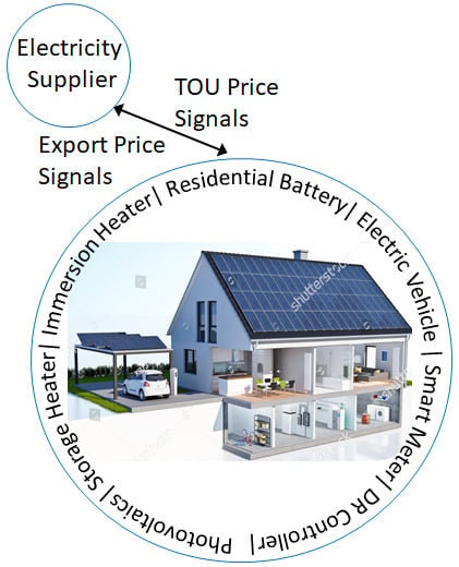
2.1. Time of Use Tariff

A TOU tariff defines variable energy prices for the customer that change typically on half-hourly intervals and are updated every day. The information about tariffs is typically sent to customers via a smartphone app. TOU tariffs require a smart meter to be installed in the household, so that consumption can be metered at the required intervals. Moreover, the customer needs to opt-in for smart meter readings at the appropriate intervals. TOU tariffs can for example provide low prices for off-peak consumption, or when cheap energy is being generated.

2.2. Controllable Electric Storage Heaters

A reduced price for off-peak consumption can be applied to electric storage heaters (Figure 2). Storage heaters accumulate heat during off-peak periods and release it when required. Efficient state-of-the-art fan assisted storage heaters with low losses have been considered. The number and size of heaters depend on house type.

2.3. Immersion Heaters

Immersion heater with storage is an electric water heater that sits inside a hot-water cylinder. Water is heated up during off-peak periods and stored in an insulated cylinder. Heating cycles can be controlled by a DR scheme. Highly insulated cylinders with negligible losses have been considered and moreover, their size is estimated to be sufficiently large to avoid the need for ‘on-peak’ top-ups of energy.

2.4. Rooftop PV

The household solar generation, where available, is assumed to offset the additional electricity load brought about by the charging of electric vehicles and/or the installation of electric heaters. Moreover, electricity generated by PV panels can help reduce the local consumption of grid electricity, and even generate an income by exporting electricity, where a local energy market is available.

2.5. Residential Battery Storage

Residential battery storage allows the storage of energy from rooftop PV or from the grid at times when the cost of electricity is reduced. The stored energy can later be used to supply local loads. Domestic battery storage technologies considered in this study are assumed to include an inverter as seen in the current market. This will allow the batteries to be readily integrated into the domestic electrical system. Their charging/discharging cycles can be controlled as part of the DR scheme.

2.6. Residential EV Charging

EV charging points with vehicle-to-grid (V2G) capability are available in some households that have adopted electric vehicles (Figure 2). The charging/discharging of EV batteries of connected vehicles can be controlled as part of the DR scheme. When the vehicle is at home, it can be used as a temporary storage resource for the household. The stored energy in the EV battery can be used to supply local loads, and it can even be exported to the grid.

2.7. Smart Thermostats and DR Controllers

The use of state-of-the-art Internet enabled automation technology, such as the If-This-Then-That (IFTTT) protocol, allows the control of key electric loads based on TOU price signals. For example, current smart thermostats, such as Tado and Nest, can already be used to control storage heaters based on TOU price signals by means of IFTTT. With the use of appropriate residential DR controllers, it will also be possible to include smart residential batteries and EV battery charging/discharging as part of the DR scheme that we envisage in this work.

2.8. Smart Meters

A smart meter is a modern type of energy meter that can send readings to the utility company via suitable communication channels, which could employ wireless or wired technologies. This can ensure more accurate energy bills relative to conventional meters with a greater sampling frequency. Smart meters provide data on energy usage to customers to help control cost and consumption. The data that smart meters send to the utility can also be used, for example, for load factor control, to analyse peak-load requirements, and for the development of pricing strategies based on consumption information dependent on the frequency and timeliness of reporting.
Currently, there are two types of smart meter in the UK: first and second-generation, which are also referred to as SMETS1 and SMETS2 (smart metering equipment technical specification), respectively. The new generation addresses several issues associated with the first generation of smart meters and provides a range of new functionality. At present only the SMETS2 smart meter can be used in conjunction with a time of use tariff.

2.9. Export of Energy to Grid

The study considers that the households participate in a local energy market with a scheme to enable customers to sell excess electricity by exporting it to the grid, the operations of which are beyond the scope of this study.

3. Demand Response Modelling

The following sub-sections describe the modelling methodology development for the above-mentioned DR technologies and methods, and the two stage optimisation algorithms:

3.1. Residential Battery

The rate of change of energy stored in battery bank is given by:
d E B t d t = η B , C P B t   if   P B t 0 P B t / η B , D   if   P B t < 0  
where EB(t) is the energy stored in battery at any instant t, PB is the power consumed (the case when PB is positive) or released (the case when PB is negative) by battery, ηB,C is the battery’s charging efficiency and ηB,D is the discharging efficiency. The energy stored in battery at any instant can be calculated by:
E B t = E B 0 + 0 t η B P B τ   d τ  
with the following initial conditions and constraints:
E B 0 th   hour = E B 24 th   hour  
P B , O P B t P B , I     t  
0 E B t E B , C     t  
ηB becomes ηB,C when PB(τ) is positive and it becomes 1/ηB,D when PB(τ) is negative. PB,O and PB,I are the output and input power ratings of battery. EB,C is the storage capacity of battery. The battery can consume power from the bus and give power to the bus. Thus, PB can be negative or positive and the bounds on the power release and consumption are conveyed by Equation (4). Note that Equation (3) is imposed to ensure that model solution is periodic, with a period of 24 h, thereby reducing the window of time over which simulations must be carried out to a single day.

3.2. Rooftop PV Electricity Generation

PV electricity generation (PPV) is defined as the electricity generated by the solar photovoltaic modules mounted at the roof of the household. The amount of power generated depends on the solar irradiance (I), reference temperature (Tref = 25 °C), reference irradiance (Iref = 1000 W/m2), area of solar cells (A), operating temperature of PV (TPV), PV efficiency at reference point (ηref = 0.1537), temperature coefficient for PV efficiency (β = −0.005 K−1), irradiance coefficient for PV efficiency (γ = 0.085) and other losses including inverter efficiency and cable/wiring losses (ηo,loss = 0.15) [28]. Thus, the power generated by rooftop PV is estimated as follows:
P P V = 1 η O , l o s s η r e f 1 + β T P V T r e f + γ ln I / I r e f I A  

3.3. Electric Storage Heater

The energy stored in the electric storage heater (ESH) at any instant can be given by:
E S H t = E S H 0 + 0 t P S H τ D S H τ d τ  
with the following initial conditions and constraints:
E S H 0 th   hour = E S H 24 th   hour  
0 P S H t P S H , I     t  
0 E S H t E S H , C     t  
where PSH is the power consumed by storage heater, DSH is the space heating demand, PSH,I is the input power rating of storage heater and ESH,C is the storage capacity of storage heater. The storage heater can consume power from the bus but cannot give power to the bus. Thus, PSH cannot be negative which is conveyed by Equation (9).

3.4. Immersion Heater

The energy stored in immersion heater (EIH) at any instant can be calculated by:
E I H t = E I H 0 + 0 t P I H τ D H W τ d τ  
with the following initial conditions and constraints:
E I H 0 th   hour = E I H 24 th   hour
0 P I H t P I H , I     t  
0 E I H t E I H , C     t  
where PIH is the power consumed by immersion heater, DHW is the hot water demand, PIH,I is the input power rating of immersion heater and EIH,C is the storage capacity of immersion heater. The immersion heater can consume power from the bus but cannot give power to the bus. Thus, PIH cannot be negative which is conveyed by Equation (13).

3.5. Battery of Electric Vehicle

The energy stored in EV battery (EEV) at any instant can be calculated by:
E E V t = E E V 0 + 0 t η E V P E V τ D E V τ d τ  
with the following initial conditions and constraints:
P E V , O P E V t P E V , I   if   t a r r < t < t d e p  
P E V t = 0   if   t d e p t t a r r  
E E V 0 th   hour = E E V 24 th   hour  
0 E E V t E E V , C     t  
where PEV is the power consumed or released by battery of EV. When PEV is positive, EV battery consumes power and when PEV is negative, EV battery releases power. ηEV becomes ηEV,C when PEV(τ) is positive and it becomes 1/ηEV,D when PEV(τ) is negative. ηEV,C is the battery’s charging efficiency and ηB,D is the discharging efficiency. DEV is the power demand for EV when EV is away from home. tarr and tdep are the arrival and departure timings of the EV to/from home respectively. PEV,O and PEV,I are the output and input power ratings of EV battery. EEV,C is the storage capacity of EV battery. The EV battery can consume power from the bus and give power to the bus when it is connected to the EV charger at the household. Thus, PEV can be negative or positive and the bounds on the power release and consumption are conveyed by Equation (16). The EV battery does not consume power from the bus nor does it give power to the bus when it is disconnected from the EV charger. Thus, the PEV is 0 for this time interval which is conveyed by Equation (17). It is assumed that EVs will follow a similar use pattern as conventional fossil fuel vehicles, with an average daily mileage for the main driver of 18.0 miles (29 km) as reported by the UK Governments Department for Transport [29]. This is approximately 5.1 kWh of the battery usage per day.

3.6. Power Consumption from the Grid and Export to the Grid

The household is able to both consume power from the grid and export power to the grid. Household power consumption/export is denoted by PG. We use a sign convention so that when PG is positive, the household consumes power from grid and when PG is negative, the household exports power to grid. Household power consumption/export can be calculated by the following power balance:
P G t + P P V t = P B t + P S H t + P I H t + P E V t D o r g t  
with the following constraint:
P G , O P G t P G , I  
where Dorg is the original electricity demand of the household before including the smart appliances. PG,O and PG,I are the bounds for the PG. The power consumption from the grid (PC) and the power export to the grid (PE) can be computed as follows:
P C t = P G t   if   P G t 0   0   if   P G t < 0  
P E t = P G t   if   P G t < 0   0   if   P G t 0  

3.7. Net Cost of Electricity

The net cost of electricity per day (COE) can be computed by subtracting the earnings due to export from the cost of consumed electricity, as follows:
C O E = 0 th   hour 24 th   hour P C t P r T O U t P E t P r E t d t  
where PrTOU(t) is the TOU price signal value at time t and PrE(t) is the export price of electricity at time t.

3.8. Objective Function

This DR approach is based on the solution of an optimisation problem for each household. The optimisation problem involves the minimisation of an objective function, which is defined as the net COE per day for each household adopting the DR scheme. This minimisation is achieved by adjusting the following decision variables: PB(t), PSH(t), PIH(t), PEV(t), EB(0), ESH(0), EIH(0), and EEV(0) during the 24 h period.

3.9. Optimisation Approach

A key underlying assumption of this study is that the DR controller receives from the energy supplier the price information in advance every day for the next 24 h period, and then it performs an optimisation that determines the optimal values of all the decision variables over the next 24 h period. This optimisation is performed with consideration of the objective function and decision variables defined in Section 3.8, along with all required constraints that are described in Section 3.1 to Section 3.7. For each household, the optimisation is performed in two stages, starting with a gradient-based nonlinear programming algorithm, and continuing the solution with a direct search optimisation approach. The first method allows it to find a good solution that satisfies all constraints relatively quickly, while the second method is able to improve the first stage solution, as it can deal with situations where the underlying functions are non-differentiable, which can occur given the nature of the functions involved in the formulation of the problem.

3.10. Aggregation

The method to aggregate power consumption of all households in the study region is described in this sub-section. The power consumption of the households that take part in DR scheme can be calculated using Equation (22). The power consumption of the households that do not take part in DR scheme is the same as the original electricity demand (Dorg). The total aggregated original power consumption of the study region (PC,org,a) and the one after the introduction of the DR scheme (PC,DR,a) can be estimated as follows:
P C ,   o r g , a t = i = 1 N D o r g i ,   t  
P C , D R , a t = i = 1 N P C i ,   t  
where N is the number of households in the study region.

3.11. Calculation of Load Power Increments

The increment in the total power consumption (ΔP) by all the households of the study region due to the adoption of new devices, technologies and DR scheme can be estimated as follows:
Δ P t = P C , D R , a t P C ,   o r g , a t  

3.12. Reduction in Energy/Fuel Bills

The reduction in daily energy/fuel bills of the participating households can be calculated by subtracting the daily bills after DR from the original daily bills before DR. The original aggregated daily bills of the participating households before DR include the original aggregated COE per day (COEorg,a), aggregated cost of heating per day by gas for on-gas households (COHongas,a), aggregated cost of heating per day by fuel for off-gas households (COHoffgas,org,a) and aggregated cost of fuel per day for vehicles (COVorg,a). The aggregated daily bills after DR include the aggregated COE per day after DR (COEDR,a) and aggregated cost of heating per day by gas for on-gas households (COHongas,a). It must be noted that the cost of heating after DR for off-gas households and the cost of fuel for vehicles after DR are already included in the COE (COEDR,a) as electric heaters and electric vehicles are used after DR. Thus, the average reduction in the energy/fuel bills per day per household (R) of the participating households can be written as follows:
R = C O E o r g , a + C O H o n g a s , a + C O H o f f g a s , o r g , a + C O V o r g , a C O E D R , a C O H o n g a s , a / n  
where n is the number of households participating in the DR scheme. Before DR, the electricity tariff of £0.14 per kWh is considered and the cost of fuel used for heating in off-gas households is considered to be £0.06 per kWh of heat delivered. For fossil fuel based vehicles, mileage of 10 miles per litre is considered with fuel cost of £1.30 per litre.

3.13. CO2 Emissions Reduction

The reduction in the CO2 emissions achieved by participating households after DR can be calculated by the addition of CO2 emissions reductions achieved by rooftop solar electricity generation, usage of electricity instead of oil for space heating in off-gas households and usage of electric vehicles instead of petrol/diesel based vehicles.
Using the 2019 UK Government GHG conversion factors [30], the following constants for CO2e were assumed. An average UK figure of 254 g CO2 emissions per kWh of grid electricity is considered. Thus, rooftop solar PV can provide 254 g CO2 emissions reduction per kWh of solar electricity generation. A figure of 270 g CO2 emissions per kWh of heat delivered by burning oil is considered, resulting in a CO2e reduction of 16 g CO2e per kWh of space heating by usage of grid electricity instead of oil. The figure will be 270 gCO2 emissions reductions per kWh of space heating if solar electricity will be used instead of oil. An average figure of 1.46 tons of CO2e emissions reductions using EV per 10,000 miles is considered.

4. Case Study: Isle of Wight Energy Autonomous Community

In this case study, the effects of applying a DR scheme in households located in the West Wight area of the IoW are investigated as part of the IoW Energy Autonomous Community (EAC). The island is located on the south coast of England, between 3 and 8 km from the mainland. At present, electricity is supplied to the IoW through two of the three interconnectors by the distribution network operator Scottish and Southern Electric Network (SSEN), with gas supplied by SGN (Figure 3).The study area on the island has been selected to represent around 50,000 inhabitants, which amounts to approximately 15,000 households in the study area, of which 3000 are not connected to the gas network. This study assumes that all participants are engaged with a single energy supplier whereby the purchase, installation and maintenance of equipment is exogenous to this study; resulting in a supplier and technology agnostic set of outputs, where we are only interested in the service and operating savings delivered.
This DR study considers both on-gas and off-gas households. Currently all off-gas households are assumed within this study to be heated using higher cost (comparatively to on gas properties), carbon-intensive fuels, such as on-peak electricity, oil and LPG. Households are assumed to adopt an appropriate subset of the aforementioned devices, technologies, or schemes (Figure 1), so that they can participate in the DR scheme. For an average household located at the study region, the estimated original electricity demand before including the proposed smart appliances [32], space heating demand [33], hot water demand, and power generated by a 3 kWp PV array [34] are shown in Figure 4, for the cases of summer and winter.
Due to variability in the sizes of households, their electricity consumptions differ. Moreover, the power ratings, sizes and number of storage heaters/immersion heaters/battery banks/PV/EV also differ for different types of households. In this study, the variability in the household size is modelled by making use of council tax bands. Our reasoning to consider council tax bands as a proxy for energy consumption is that council tax bands correlate well with the size of the property, given this tax was established on the basis of house price at a particular year in the past, and for a given region, house prices are correlated to size. Moreover, size correlates to energy consumption since a greater household volume requires a greater amount of energy for heating during winter months. There is also increased electricity consumption due to lighting and the higher capacity for occupants in a bigger household. A greater number of occupants means a greater hot water and electricity consumption. The percentage of households in the IoW that belongs to Council Tax Band A is 14.42%. The respective values for Band B, C, D, E, F, G, and H are 25.57%, 24.21%, 19.00%, 10.06%, 4.48%, 2.06%, and 0.2%. Based on the given distribution of households in the council tax bands, the household of Band C represents the average household. The original electricity demand, space heating demand and water heating demands per household for Band A, B, D, E, F, G, and H are 0.667, 0.833, 1.167, 1.333, 1.667, 2, and 2.333 times than that of B and C.
The increments in the total power consumption by all the households of the study region due to the adoption of new devices, technologies and DR scheme are computed within the model described above. The corresponding CO2 emissions reduction due to the decarbonisation and reduction in bills for the participating households are also computed. The resulting load power increments are divided in equal parts into the two substations (Substations A and B) that serve the region of study (Figure 3). Each substation has two power transformers whose secondary is a common bus which represents the connection point to the distribution feeders that supply the region of study. Subsequently, the power increments for each substation are added to the known demand profiles for the corresponding secondary buses. Using a distribution network model for the IoW, along with a load flow software tool developed by the University of Newcastle based on MATPOWER (exogenous to the model described within this paper [35]), secondary voltages and apparent power through transformers of substations after the introduction of DR scheme are computed and compared against the original values (note that at present, it is not possible to display the original values before the adoption of DR scheme due to an embargo on the original base data) before the adoption of DR scheme. Moreover, the apparent power flows through the undersea cable interconnectors with the mainland before and after the implementation of DR are analysed, and the increments in the apparent power through the interconnectors are reported. The results are computed and analysed for six decarbonisation scenarios based on the season, and different adoption levels of DR scheme and electric vehicles.
The study is based on the following assumptions:
  • Table 1 shows the specifications assumed in this study for the rooftop PV installation, storage heaters, immersion heaters, battery banks, and electric vehicles for all the household types.
  • The devices currently available in the market have been considered, and have sized them appropriately for the corresponding household type.
  • With regard to the specifications of the electric vehicle battery capacity, we assumed that smaller properties that have an electric vehicle will have a Nissan Leaf (or similar) with a battery capacity of 30 kWh, while larger households that have an electric vehicle will have a Tesla Model S (or similar) with a battery capacity of 70 kWh.
  • In all cases, we assumed an EV charger with a power rating of 10 kW. The larger power rating for the EV charger (compared to the entry level of 3 kW) allows greater flexibility for vehicle-to-grid (V2G) applications.
  • The specification of the rooftop PV installation is determined on the basis of household size, considering typical installations in the UK. It is assumed that only the properties participating in the DR scheme have a PV installation.
  • Each household size (as represented by the council tax band) is assumed to have devices with different ratings.
  • Time of use tariffs and export tariffs employed are shown in Table 2, and remain fixed within their time ranges as discussed within private communication with Lumeanza GmBH (Lumenaza GmBH is an SME that specialises in developing specialist algorithms and software for the sale and supply of locally produced renewable energy) [36].
  • In the scenarios described within Section 5, the central figure of 10% EV adoption assumes projected EV passenger vehicle penetration level in the UK for 2025 [37]. It is assumed in the scenarios that all houses that have an EV are participating in the DR scheme, and that there is only one EV in each of those households. Note that not all households that are part of the DR scheme are assumed to have an EV.
  • The demand data and network topology used in load flow studies correspond to the year 2017.

5. Results and Discussion

The following six decarbonisation scenarios have been considered to estimate the total power consumption by 15,000 households in the study region, apparent power flows through transformers, voltages at transformers, apparent power flows through interconnectors, CO2 emissions reduction and reduction in bills under different scenarios based on the season, percentage of the households adopting DR scheme and percentage of households having electric vehicles. With regard to the level of adoption of the DR scheme, we consider a base scenario of 40% adoption in the study region, and evaluate sensitivity by considering a higher (60%) level of adoption, and a lower (20%) level of adoption. In relation to the level of adoption of electric vehicles, we consider a central case of 10% adoption in the study region and evaluate sensitivity by considering lower EV adoption (5%), and higher EV adoption (15%). Producing the following scenarios in Table 3.

5.1. Scenario 1: Winter, DR 40%, EV 10%

The increments in the total power demand by 15,000 households over a 24 h period due to the adoption of DR and new devices are computed for winter month when 40% of the households of the study region adopt DR and 10% adopt an EV. It is found that there is an increment of 44 MWh/day. However, due to the decarbonisation, CO2 emissions reduction of 16 tons/day and average reduction in bills of 28% are achieved by the participating households for this scenario.
The apparent power flows through transformers after implementing DR are plotted in Figure 5 for both substations. The results show that the DR optimization has shifted the electricity demand towards late night when electricity is cheaper. The minimum apparent power flows after DR are decreased to 2.1 and 1.3 MVA for substations A and B respectively. The maximum apparent power flows after DR are increased to 15.4 and 14.2 MVA for substations A and B respectively. It is seen that even after adopting the DR and new devices, the maximum apparent power flows are 51% and 47% of the combined transformer power rating of substations A and B respectively.
Secondary voltages at transformers of both substations after the introduction of DR scheme are presented in Figure 6a. It can be seen that the minimum and maximum voltages after DR at transformers in substation A are 0.872 and 0.965 p.u., respectively. For transformers at substation B, these values are 0.859 and 0.968 p.u., respectively. It can be seen that there are instances when the voltages are 12.8% and 14.1% below the nominal voltages for transformers at substations A and B respectively. These voltages are clearly not acceptable from an operational perspective, but there are relatively easy ways of bringing those voltages to the allowed range of +/− 6% of the nominal voltage, including the adjustment of transformer taps and reactive compensation.
The apparent power flows through the interconnectors after the implementation of DR are analysed. It is found that the maximum apparent power flow at the interconnectors after DR is decreased by 2.9%. The increments in the apparent power flow through the inter-connectors after the implementation of DR are also plotted in Figure 6b. Note that the apparent power flows through the interconnectors tend to increase between 0:00 and 7:00 (hence the positive increments) because of increased consumption in the study region driven by low electricity prices, while they decrease (negative increments) during the rest of the day partly as a result of PV generation in participating households, export of electricity from the households to the grid, the use of energy storage, and higher electricity prices.

5.2. Scenario 2: Summer, DR 40%, EV 10%

The increments in the total power demand by 15,000 households over a 24 h period due to adoption of DR and new devices are computed for summer month when 40% of the households of the study region adopt DR and 10% adopt an EV. It is found that there is a decrement of 19 MWh/day due to excess solar electricity generation. Due to the decarbonisation, CO2 emissions reduction of 23 tons/day and average reduction in bills of 93% are achieved by the participating households for this scenario.
The apparent power flows through transformers after implementing DR are plotted in Figure 7 for both substations. The results show that the minimum apparent power flows after DR are decreased to 0.9 and 1.1 MVA for substations A and B respectively. The maximum apparent power flow after DR is increased to 7.0 MVA for substations A and B respectively. It is seen that even after adopting the DR and new devices, the maximum apparent power flow is 23% of the combined transformer power rating of substations A and B.
Secondary voltages at transformers of both substations after the introduction of the DR scheme are presented in Figure 8a. It can be seen that the minimum and maximum voltages after DR at transformers in substation A are 0.934 and 0.976 p.u., respectively. For transformers at substation B, these values are 0.926 and 0.974 p.u. respectively. It can be seen that there are instances when the voltages are 6.6% and 7.4% below the nominal voltages for transformers at substations A and B respectively.
The apparent power flows through the interconnectors after the implementation of DR are analysed. It is found that the maximum apparent power flow at the interconnectors after DR is decreased by 0.9%. The increment in the apparent power flow through the inter-connectors after the implementation of DR is also plotted in Figure 8b.
Aggregated power export from the participating households after the implementation of DR for scenario 2 is plotted in Figure 9. Note that the peak value of 6.4MW is about 10% of the installed large-scale solar PV generation capacity on the island.

5.3. Scenario 3: Winter, DR 60%, EV 10%

The increments in the total power demand by 15,000 households over a 24 h period due to the adoption of DR and new devices are computed for winter month when 60% of the households of the study region adopt DR and 10% adopt an EV. It is found that there is an increment of 59 MWh/day. However, due to the decarbonisation, CO2 emissions reduction of 22 tons/day and average reduction in bills of 27% are achieved by the participating households for this scenario.
The apparent power flows through transformers after implementing DR are plotted in Figure 10 for both substations. The results show that the minimum apparent power flows after DR are decreased to 1.2 and 0.4 MVA for substations A and B respectively. The maximum apparent power flows after DR are increased to 20.8 and 19.6 MVA for substations A and B respectively. It can be seen that even after adopting the DR and new devices, the maximum apparent power flows are 69% and 65% of the combined transformer power rating of substations A and B respectively.
Secondary voltages at transformers of both substations after the introduction of DR scheme are presented in Figure 11a. It can be seen that the minimum and maximum voltages after DR at transformers in substation A are 0.820 and 0.971 p.u., respectively. For transformers at substation B, these values are 0.798 and 0.974 p.u., respectively. It can be seen that there are instances when the voltages are 18.0% and 20.2% below the nominal voltages for transformers at substations A and B, respectively.
The apparent power flows through the interconnectors after the implementation of DR are analysed. It is found that the maximum apparent power flow at the interconnectors after DR is decreased by 4.3%. The increment in the apparent power flow through the inter-connectors after the implementation of DR is also plotted in Figure 11b.

5.4. Scenario 4: Winter, DR 20%, EV 10%

The increments in the total power demand by 15,000 households over a 24 h period due to the adoption of DR and new devices are computed for winter month when 20% of the households of the study region adopt DR and 10% adopt an EV. It is found that there is an increment of 28 MWh/day. However, due to the decarbonisation, CO2 emissions reduction of 10 tons/day and average reduction in bills of 37% are achieved by the participating households for this scenario.
The apparent power flows through transformers after implementing DR are plotted in Figure 12 for both substations. The results show that the minimum apparent power flows after DR are decreased to 3.1 and 2.2 MVA for substations A and B respectively. The maximum apparent power flow after DR are increased to 10.7 and 9.5 MVA for substations A and B respectively. It can be seen that even after adopting the DR and new devices, the maximum apparent power flows are 35% and 32% of the combined transformer power ratings of substation A and B respectively.
Secondary voltages at transformers of both substations after the introduction of DR scheme are presented in Figure 13a. It can be seen that the minimum and maximum voltages after DR at transformers in substation A are 0.913 and 0.960 p.u., respectively. For transformers at substation B, these values are 0.906 and 0.961 p.u., respectively. It can be seen that there are instances when the voltages are 8.7% and 9.4% below the nominal voltages for transformers at substations A and B, respectively.
The apparent power flows through the interconnectors after the implementation of DR are analysed. It is found that the maximum apparent power flow at the interconnectors after DR is decreased by 1.5%. The increment in the apparent power flow through the inter-connectors after the implementation of DR is also plotted in Figure 13b.

5.5. Scenario 5: Winter, DR 40%, EV 5%

The increments in the total power demand by 15,000 households over a 24 h period due to the adoption of DR and new devices are computed for winter month when 40% of the households of the study region adopt DR and 5% adopt an EV. It is found that there is an increment of 37 MWh/day. However, due to the decarbonisation, CO2 emissions reduction of 14 tons/day and average reduction in bills of 23% are achieved by the participating households for this scenario.
The apparent power flows through transformers after implementing DR are plotted in Figure 14 for both substations. The results show that the minimum apparent power flows after DR are decreased to 2.2 and 1.3 MVA for substations A and B respectively. The maximum apparent power flows after DR are increased to 14.9 and 13.7 MVA for substations A and B respectively. It can be seen that even after adopting the DR and new devices, the maximum apparent power flows are 50% and 46% of the combined transformer power ratings of substations A and B respectively.
Secondary voltages at transformers of both substations after the introduction of DR scheme are presented in Figure 15a. It can be seen that the minimum and maximum voltages after DR at transformers in substation A are 0.875 and 0.965 p.u., respectively. For transformers at substation B, these values are 0.862 and 0.968 p.u., respectively. It can be seen that there are instances when the voltages are 12.5% and 13.8% below the nominal voltages for transformers at substations A and B, respectively.
The apparent power flows through the interconnectors after the implementation of DR are analysed. It is found that the maximum apparent power flow at the interconnector after DR is decreased by 2.9%. The increment in the apparent power flow through the inter-connectors after the implementation of DR is also plotted in Figure 15b.

5.6. Scenario 6: Winter, DR 40%, EV 15%

The increments in the total power demand by 15,000 households over a 24 h period due to the adoption of DR and new devices are computed for winter month when 40% of the households of the study region adopt DR and 15% adopt an EV. It is found that there is an energy demand increment of 50 MWh/day. However, due to the decarbonization, CO2 emissions reduction of 18 tons/day and average reduction in bills of 33% are achieved by the participating households for this scenario.
The apparent power flows through transformers after implementing DR are plotted in Figure 16 for both substations. The results show that the minimum apparent power flows after DR are decreased to 2.1 and 1.3 MVA for substations A and B respectively. The maximum apparent power flows after DR are increased to 15.8 and 14.6 MVA for substations A and B respectively. It can be seen that even after adopting the DR and new devices, the maximum apparent power flows are 53% and 49% of the combined transformer power ratings of substations A and B respectively.
Secondary voltages at transformers of both substations after the introduction of the DR scheme are presented in Figure 17a. It can be seen that the minimum and maximum voltages after DR at transformers in substation A are 0.868 and 0.966 p.u., respectively. For transformers at substation B, these values are 0.853 and 0.968 p.u. respectively. It can be seen that there are instances when the voltages are 13.2% and 14.6% below the nominal voltages for transformers at substations A and B, respectively.
The apparent power flows through the interconnectors after the implementation of DR are analysed. It is found that the maximum apparent power flow at the interconnectors after DR is decreased by 2.9%. The increment in the apparent power flow through the inter-connectors after the implementation of DR is also plotted in Figure 17b.

5.7. Sensitivity Analysis

In this section, we briefly discuss the sensitivity of key variables to changes in the assumed adoption level of the DR scheme, changes in the assumed adoption level of electric vehicles, and also with respect to the season.
Figure 18a shows that the increment in electricity demand increases linearly with the level of adoption of the DR scheme, as do the CO2 emissions reductions and maximum transformer loading at the substations. Moreover, the minimum voltage level at the secondary of the transformers at substations decreases with increase in the level of adoption of the DR scheme. A similar sensitivity is noted with changes in the level of adoption of electric vehicles, as shown in Figure 18b.
Figure 19 shows that the electricity demand due to the demand response scheme and new devices increases significantly from summer to winter, as does the maximum transformer loading at the substations. The minimum voltage at the secondary of transformers at substations decreases visibly. It can also be seen that the CO2 emissions reduction is higher in summer due to higher solar electricity generation.
The results will also be sensitive to many of the assumptions and choices made, including for example the choice of the objective function for DR optimisation, the time of use tariff, and the export price of electricity. These are pre-determined by the user and within the reported scenarios remain fixed.

5.8. Discussion

As a case study, the effects of applying a DR scheme in households located in the West Wight area of the IoW are investigated. The estimated total power demand by 15,000 households in the study region after implementing DR is compared against the original estimated power demand before DR. The increment in the total power demand is calculated, and its effects at key voltages and power flows are determined using a model of the distribution network of the IoW and a load flow software tool. Specifically, secondary voltages and power flows through the transformers located at substations after the introduction of the DR scheme are computed. Moreover, the apparent power flows through interconnectors between the IoW and the mainland after the implementation of DR are analysed, and the increment in the total apparent power flow is reported. The corresponding CO2 emissions reduction and reduction in energy/fuel bills for the participating households are also computed. The results show that:
  • An average reduction in energy/fuel bills of 60% per annum can be achieved if 40% of the households adopt DR and 10% adopt an EV.
  • The respective increments in the total electricity demands are 28, 44 and 59 MWh/day in winter if 20%, 40%, and 60% of the households adopt DR and 10% adopt an EV. The corresponding CO2 emissions reductions are 10, 16, and 22 tons per day.
  • The respective increment in the total electricity demand is 44 MWh/day in winter and a decrement is 19 MWh/day in summer if 40% of the households adopt DR and 10% adopt an EV. The corresponding CO2 emissions reductions are 16 and 23 tons per day.
  • The respective increments in the total electricity demands are 37, 44 and 50 MWh/day in winter if 5%, 10%, and 15% of the households adopt an EV and 40% adopt DR. The corresponding CO2 emissions reductions are 14, 16, and 18 tons per day.
  • After implementing the DR scheme, the respective maximum apparent power flows through transformers are 35%, 51%, and 69% of the combined transformer power rating for 20%, 40%, and 60% DR adoption scenarios.
  • There are instances when the secondary voltages are 9.4%, 14.1%, and 20.2% below the nominal voltages for transformers at substations for 20%, 40%, and 60% DR adoption scenarios. These voltages are clearly not acceptable from an operational perspective, but there are relatively easy ways of bringing those voltages to the allowed range of +/− 6% of the nominal voltage, including the adjustment of transformer taps and the use of reactive compensation.
  • The maximum apparent power flows through the interconnectors after DR are decreased by 0.8%, 2.2%, and 3.6% for 20%, 40%, and 60% DR adoption scenarios.
  • Aggregated power export from the participating households after the implementation of DR is also estimated. It is noted that for scenario 2 (summer, 40% adoption of DR, 10% adoption of EV), the peak value of export is about 6.4 MW, which is about 10% of the installed large-scale solar PV generation capacity on the island.
Through utilising a community wide area with multiple household sizes and various compositions of DR technologies this work builds upon the current literature focusing primarily on single technologies within an individual domestic setting [2,3,4,5,8]. This work highlights the positive impact that integrating intelligent DR systems can have on operating costs and GHG emissions on a community scale.
Within the model presented, several key limitations exist concerning the EV charging infrastructure. At present the model does not consider vehicle charging and discharging during the day when there is peak supply of renewable generation and the ability to utilise excess stored capacity, reducing the need to charge during the night when renewable output diminishes. This model does not address the embed CO2 and financial/economic costs associated with the removal of non-DR technologies and the installation of new equipment.
The sensitivity analysis whereby EV ownership remains constant and participation within the scheme increases from 20% to 40% and 60% shows a decrease in household savings from 37%, 28%, to 27% respectively. This is due to the fact that the high savings produced by owning an EV are diluted by increased participation of non EV owners.

6. Conclusions

In this work, a two-stage optimisation DR model applied to complete households is described. The model incorporates multiple potential DR functions that have been widely reported within the literature; including electric vehicles (EV), rooftop PV, the ability to export electricity to generate revenue, time of use tariffs, smart battery storage, electric storage heaters, immersion water heaters, smart meters and DR controllers. This DR model can be used to provide valuable information for energy systems decision and policy makers, particularly when used to analyse the systemic effects of possible future national or regional policies and technologies.
From the Isle of Wight Energy Autonomous Community case study three main conclusions can be drawn:
  • All scenarios showed a reduction in energy/transport fuel-bills of between 23% and 93%. Within the case study outputs, it is clear that increasing EV ownership can lead to a greater reduction in overall combined energy costs, particularly in the summer season. This is likely due to a combined ability to generate a revenue through the export of excess energy that offsets total costs, with a reduction in heating costs for off-gas properties by using electricity instead of fossil fuels.
  • All scenarios demonstrate a reduction in the climate impacts with between 10 to 23 tons per day of CO2e between the interventions. It is likely that that EV owners experience both a greater saving on total fuel bills and a greater reduction in CO2e emissions.
  • In all scenarios, the apparent power flows at each substation remain below their operating capacities, showing little to no rebound effect from the uptake of DR technologies. This would enable a large uptake of DR without increasing the cost to the DNO.
This work demonstrates the potential beneficial impacts that a DR can have both for the customer in terms of financial savings and for the community at large through the reduction in GHG emissions. Minimal uptake enabled savings is exhibited by all engaged customers, showing that there is scalability in the integration of these methodologies and is not dependent on a significant initial uptake. However, this study does not take into consideration the embedded cost of the DR technologies, which are at present exogenous to the model inputs. It is likely that this would result in significantly reduced financial savings if the individuals were to purchase the equipment. It is assumed that the technology would be adopted as best available technology as existing hardware is upgraded/replaced.
Financial savings within this study are dependent on the use of EVs, with lower DR participation (20%) and EV ownership at 10% receiving the greatest financial savings of 37%, compared to 28% and 27% respectively for the 40% and 60% participation rates. This highlights the importance of incorporating EV charging into future policies, regulations, and business models for distributed energy services.
The DR modelling approach is deterministic and does not account for uncertainty in the model input, and only considers uncertainty through the uptake rate of DR and EV ownership within the communities. This can be improved through the implementation of stochastic analysis, although this would also require significantly more data on input variables and would become computationally intensive due to the non-linear aspect of the model. The current model can enable dynamic pricing based on generation and demand profiles. However, in this instance, the values are fixed as the pricing is outside of the remit of this study. The model and the case study currently do not consider the following: embedded costs/CO2e of new technologies, dynamic EV charging/discharge and the virtual power plant model. Future work will enable the integration of these functions, with the ability to disaggregate customer types to determine how both EV and non-EV owners benefit, as well as prosumer/non-prosumer members. Future iterations will also enable the input of commercial and industrial consumers as well as community and local energy production schemes.
Transitioning towards a smart local energy system will require the engagement and cooperation of all stakeholders, primarily the customers and energy suppliers. Initially, due to the inherently high technology costs associated with the adoption and deployment of DR schemes, there will likely need to be policies and regulations that will incentivise uptake. This work shows that there are both financial and environmental benefits associated with a low uptake rate of DR, which could enable small energy supply companies to create a competitive service. However, further research is required to understand how dynamic tariffs, financial savings through grid balancing and potential carbon credits (among others) can be utilised to offset potentially high technology costs and encourage uptake.

Author Contributions

Conceptualisation, V.B. and S.K.; methodology, S.K. and V.B.; software, S.K., V.B., A.A., and D.G.; formal analysis, S.K., V.B., J.M.F., A.A., and D.G.; investigation, S.K., V.B., J.M.F., A.A., and D.G.; writing—original draft preparation, S.K. and V.B.; writing—review and editing, K.R., S.K., V.B., J.M.F., A.A., D.G., D.H., and J.F.; project co-ordinator, J.F and D.H.; supervision, V.B. All authors have read and agreed to the published version of the manuscript.

Funding

This research received funding from Innovate UK Smart Local Energy Systems Concepts 133798, -project entitled “Isle Of Wight Energy Autonomous Community” (Grant Number: 17660).

Acknowledgments

The valuable inputs and thoughtful conversations with the project partner Tereza Borges (Lumenaza GmBH) and other project partners are greatly acknowledged.

Conflicts of Interest

The authors declare no conflict of interest.

Nomenclature

CO2eCarbon dioxide equivalent
COECost of electricity
COHCost of heating
COVCost of vehicle
DNODistribution network operator
DRDemand response
EACEnergy autonomous community
EVElectric vehicle
HEMSHome energy management system
IHImmersion heater
IoWIsle of Wight
PVPhotovoltaics
SHStorage heater
SMETS1(2)Smart metering equipment technical specification
TOUTime of use
TOUTTime of use tariff
V2GVehicle to grid

References

  1. Torriti, J. Price-based demand side management: Assessing the impacts of time-of-use tariffs on residential electricity demand and peak shifting in Northern Italy. Energy 2012, 44, 576–583. [Google Scholar] [CrossRef]
  2. Kusakana, K. Energy management of a grid-connected hydrokinetic system under Time of Use tariff. Renew. Energy 2017, 101, 1325–1333. [Google Scholar] [CrossRef]
  3. Anda, M.; Temmen, J. Smart metering for residential energy efficiency: The use of community based social marketing for behavioural change and smart grid introduction. Renew. Energy 2014, 67, 119–127. [Google Scholar] [CrossRef]
  4. Aghaei, J.; Alizadeh, M.I. Demand response in smart electricity grids equipped with renewable energy sources: A review. Renew. Sustain. Energy Rev. 2013, 18, 64–72. [Google Scholar] [CrossRef]
  5. Boroojeni, K.G.; Amini, M.H.; Iyengar, S.S. Smart Grids: Security and Privacy Issues; Springer International Publishing: Cham, Switzerland, 2017. [Google Scholar]
  6. Rushby, T.; Anderson, B.; Bahaj, A.; James, P. SAVE SDRC 2.2: SAVE Updated Customer Model. 2017. Available online: https://www.researchgate.net/publication/325795355_SAVE_SDRC_22_SAVE_Updated_Customer_Model (accessed on 29 October 2019).
  7. Drysdale, B.; Wu, J.; Jenkins, N. Flexible demand in the GB domestic electricity sector in 2030. Appl. Energy 2015, 139, 281–290. [Google Scholar] [CrossRef] [Green Version]
  8. Parag, Y.; Sovacool, B.K. Electricity market design for the prosumer era. Nat. Energy 2016, 1, 16032. [Google Scholar] [CrossRef]
  9. The Committee on Climate Change. Reducing UK Emissions–2019 Progress Report to Parliament. Available online: https://www.theccc.org.uk/publication/reducing-uk-emissions-2019-progress-report-to-parliament/#outline (accessed on 29 October 2019).
  10. Department for Business, Energy and Industrial Strategy. Barriers and Benefits of Home Energy Controller Integration. Available online: https://www.gov.uk/government/publications/barriers-and-benefits-of-home-energy-controller-integration (accessed on 14 March 2019).
  11. Kolenc, M.; Ihle, N.; Gutschi, C.; Nemcek, P.; Breitkreuz, T.; Godderz, K.; Suljanovic, N.; Zajc, M. Virtual power plant architecture using OpenADR 2.0b for dynamic charging of automated guided vehicles. Int. J. Electr. Power Energy Syst. 2019, 104, 370–382. [Google Scholar] [CrossRef]
  12. Mi, X.; Qian, F.; Zhang, Y.; Wang, X. An empirical characterization of IFTTT: Ecosystem, usage, and performance. In Proceedings of the 2017 Internet Measurement Conference (IMC), London, UK, 1–3 November 2017; ACM Digital Library: New York, NY, USA, 2017; pp. 398–404. [Google Scholar]
  13. Ghiani, E.; Giordano, A.; Nieddu, A.; Rosetti, L.; Pilo, F. Planning of a Smart Local Energy Community: The Case of Berchidda Municipality (Italy). Energies 2019, 12, 4629. [Google Scholar] [CrossRef] [Green Version]
  14. Kirpes, B.; Mengelkamp, E.; Schaal, G.; Weinhardt, C. Design of a Microgrid Local Energy Market on a Blockchain-Based Information System. it-Inf. Technol. 2019, 61, 87–99. [Google Scholar] [CrossRef]
  15. Kilkki, O.; Alahaivala, A. Optimized control of price-based demand response with electric storage space heating. IEEE Trans. Ind. Inform. 2015, 11, 281–288. [Google Scholar] [CrossRef]
  16. Qazi, H.W.; Flynn, D. Demand side management potential of domestic water heaters and space heaters. IFAC Proc. Vol. 2012, 45, 693–698. [Google Scholar] [CrossRef] [Green Version]
  17. Arteconi, A.; Polonara, F. Assessing the Demand Side Management Potential and the Energy Flexibility of Heat Pumps in Buildings. Energies 2018, 11, 1846. [Google Scholar] [CrossRef] [Green Version]
  18. Wu, Z.; Tazvinga, H.; Xia, X. Demand side management of photovoltaic-battery hybrid system. Appl. Energy 2015, 148, 294–304. [Google Scholar] [CrossRef] [Green Version]
  19. Moura, P.S.; Almeida, A.T. The role of demand-side management in the grid integration of wind power. Appl. Energy 2010, 87, 2581–2588. [Google Scholar] [CrossRef]
  20. Azeez, N.T.; Atikol, U. Utilizing demand-side management as tool for promoting solar water heaters in countries where electricity is highly subsidized. Energy Sources Part B Econ. Plan. Policy 2019, 14, 34–48. [Google Scholar] [CrossRef]
  21. Laicane, I.; Blumberga, D.; Blumberga, A.; Rosa, M. Reducing household electricity consumption through demand side management: The role of home appliance scheduling and peak load reduction. Energy Procedia 2015, 72, 222–229. [Google Scholar] [CrossRef] [Green Version]
  22. Thomas, E.; Sharma, R.; Nazarathy, Y. Towards demand side management control using household specific Markovian models. Automatica 2019, 101, 450–457. [Google Scholar] [CrossRef]
  23. Reka, S.S.; Ramesh, V. A demand response modeling for residential consumers in smart grid environment using game theory based energy scheduling algorithm. Ain Shams Eng. J. 2016, 7, 835–845. [Google Scholar] [CrossRef] [Green Version]
  24. Ghazvini, M.A.F.; Soares, J.; Abrishambaf, O.; Castro, R. Demand response implementation in smart households. Energy Build. 2017, 143, 129–148. [Google Scholar] [CrossRef] [Green Version]
  25. Setlhaolo, D.; Xia, X.; Zhang, J. Optimal scheduling of household appliances for demand response. Electr. Power Syst. Res. 2014, 116, 24–28. [Google Scholar] [CrossRef]
  26. Silva, A.; Marinheiro, J.; Cardoso, H.L.; Oliveira, E. Demand-side management in Power Grids: An ant colony optimization approach. In Proceedings of the IEEE 18th International Conference on Computational Science and Engineering, Porto, Portugal, 21–23 October 2015. [Google Scholar]
  27. Smart Energy Demand Coalition. Explicit and Implicit Demand-Side Flexibility: Complementary Approaches for an Efficient Energy System. Available online: https://www.smarten.eu/wp-content/uploads/2016/09/SEDC-Position-paper-Explicit-and-Implicit-DR-September-2016.pdf (accessed on 16 January 2020).
  28. Khanna, S.; Sundaram, S.; Reddy, K.S.; Mallick, T.K. Performance analysis of perovskite and dye-sensitized solar cells under varying operating conditions and comparison with monocrystalline silicon cell. Appl. Therm. Eng. 2017, 127, 559–565. [Google Scholar] [CrossRef]
  29. Department for Transport. Transport Statistics for Great Britain 2017. Available online: https://assets.publishing.service.gov.uk/government/uploads/system/uploads/attachment_data/file/664323/tsgb-2017-print-ready-version.pdf (accessed on 1 November 2019).
  30. Department for Business Energy & the Industrial Strategy. 2019 Government Greenhouse Gas Conversion Factors for Company Reporting. Available online: https://assets.publishing.service.gov.uk/government/uploads/system/uploads/attachment_data/file/829336/2019_Green-house-gas-reporting-methodology.pdf (accessed on 29 October 2019).
  31. Grontmij. Isle of Wight Renewable Energy Resource Investigation Review of Potential for Connection of Embedded Generation Sources into Existing Public Electricity Supply Distribution System. Available online: http://www.iwight.com/documentlibrary/download/grid-connection-study (accessed on 29 October 2019).
  32. Elexon Ltd. Electricity User Load Profiles by Profile Class. EDC Dataset Serial Number EDC0000041. 2017. Available online: https://data.ukedc.rl.ac.uk/browse/edc/efficiency/residential/LoadProfile/Load_Profiles.pdf (accessed on 4 April 2019).
  33. Watson, S.D.; Lomas, K.J.; Buswell, R.A. Decarbonising domestic heating: What is the peak GB demand? Energy Policy 2019, 126, 533–544. [Google Scholar] [CrossRef]
  34. European Commission, Joint Research Centre, Institute for Environment and Sustainability. Weather Data. Photovoltaic Geographical Information System. Available online: http://re.jrc.ec.europa.eu/pvgis/apps4/pvest.php (accessed on 18 April 2019).
  35. Zimmerman, R.D.; Murillo-Sánchez, C.E.; Thomas, R.J. MATPOWER: Steady-state operations, planning, and analysis tools for power systems research and education. IEEE Trans. Power Syst. 2010, 26, 12–19. [Google Scholar] [CrossRef] [Green Version]
  36. Borges, T.; Böhmer, B.; Lumenaza GmBH, Berlin, Germany. Personal communication, 2019.
  37. Baringa Partners LLP. Is the UK Ready for Electric Cars? Available online: https://www.baringa.com/BaringaWebsite/media/BaringaMedia/PDF/Is-the-UK-ready-for-Electric-Cars-FINAL-WEB.pdf (accessed on 18 April 2019).
Figure 1. (a) On-gas and (b) off-gas households adopting demand response scheme and EV. TOU: time of use, EV: electric Vehicle, DR: demand Response.
Energies 13 00541 g001
Figure 2. Illustration of electrical bus in the household, the different elements connected to it and the directions of power flows. The vertical line represents a connection bus in the households, the arrows indicate the possible direction(s) of the power flow and the switch in the electric vehicle indicates that it can be connected or disconnected at different times of the day.
Energies 13 00541 g002
Figure 3. Isle of Wight (IoW) electrical distribution system-network map. The IoW study area is highlighted in green. Locations of assets and routes of overhead lines, underground cables and submarine cables are approximate indications for information only. PV—Photovoltaic, MW—Megawatt, kV—Kilovolt. Image produced using data from Grontmij (2010) [31].
Energies 13 00541 g003
Figure 4. (a) Original electricity demand before including the smart appliances, (b) space heating demand, (c) water heating demand, and (d) power generated by 3 kWp PV array for an average household located at the study region.
Energies 13 00541 g004aEnergies 13 00541 g004b
Figure 5. Apparent power flows through transformers after the introduction of DR scheme for scenario 1.
Energies 13 00541 g005
Figure 6. (a) Secondary voltage at transformers of both substations and (b) increment in apparent power flow through inter-connectors after the implementation of DR for scenario 1.
Energies 13 00541 g006
Figure 7. Apparent power flows through transformers after the introduction of DR scheme for scenario 2.
Energies 13 00541 g007
Figure 8. (a) Secondary voltage at transformers of both substations and (b) increment in apparent power flow through inter-connectors after the implementation of DR for scenario 2.
Energies 13 00541 g008
Figure 9. Aggregated power export from the participating households after the implementation of DR for scenario 2 (summer, DR adoption level of 40%, EV adoption level of 10%).
Energies 13 00541 g009
Figure 10. Apparent power flows through transformers after the introduction of DR scheme for scenario 3.
Energies 13 00541 g010
Figure 11. (a) Secondary voltage at transformers of both substations and (b) increment in apparent power flow through inter-connectors after the implementation of DR for scenario 3.
Energies 13 00541 g011
Figure 12. Apparent power flows through transformers after the introduction of DR scheme for scenario 4.
Energies 13 00541 g012
Figure 13. (a) Secondary voltage at transformers of both substations, and (b) increment in apparent power flow through inter-connectors after the implementation of DR for scenario 4.
Energies 13 00541 g013
Figure 14. Apparent power flows through transformers after the introduction of DR scheme for scenario 5.
Energies 13 00541 g014
Figure 15. (a) Secondary voltage at transformers of both substations and (b) increment in apparent power flow through inter-connectors after the implementation of DR for scenario 5.
Energies 13 00541 g015
Figure 16. Apparent power flows through transformers after the introduction of DR scheme in the study region for scenario 6.
Energies 13 00541 g016
Figure 17. (a) Secondary voltage at transformers of both substations and (b) increment in apparent power flow through inter-connectors after the implementation of DR for scenario 6.
Energies 13 00541 g017
Figure 18. Sensitivity of key variables with respect to the level of adoption of the (a) DR scheme for winter and EV adoption level at 10% and (b) EV for winter and DR adoption level at 40%.
Energies 13 00541 g018
Figure 19. Sensitivity of key variables with respect to the season for DR adoption level at 40% and EV adoption level at 10%.
Energies 13 00541 g019
Table 1. Devices specifications.
Gas Connection TypeCouncil Tax BandPV Peak Power Rating (kW)SH Total Storage Capacity (kWh)SH Total Input Power Rating (kW)SH Total Heat Output Rating (kW)IH Power Rating (kW)Hot Water Cylinder Volume (L)IH Storage Capacity (kWh)Battery Storage Capacity (kWh)Battery Power Rating (kW)EV Battery Capacity (kWh)EV Battery Charger Power Rating (kW)
On gasA200000030.53010
B2.500000030.53010
C30000004.82.43010
D3.50000004.82.43010
E40000004.82.43010
F50000004.82.43010
G60000007.237010
H70000001457010
Off gasA232.84.72.131204.9030.53010
B2.543.76.22.831506.1330.53010
C354.67.83.531807.354.82.43010
D3.565.59.44.231807.354.82.43010
E476.410.94.931807.354.82.43010
F587.412.55.631807.354.82.43010
G6109.215.6732108.587.237010
H7131.018.78.4325010.211457010
Table 2. Time of use and export tariffs [36] (wholesale price, WHP, for electricity is 6.1 p/kWh).
TimeTOU Tariff Summer (p/kWh)TOU Tariff Winter (p/kWh)Export Tariff Summer (p/kWh)Export Tariff Winter (p/kWh)
11 PM–6 AM7.918.5WHP + 0.5 pWHP + 0.6 p
6 AM–10 AM16.2717.5WHP + 0.1 pWHP + 0.6 p
10 AM–4 PM1314WHP − 0.5 pWHP + 0.4 p
4 PM–11 PM32.5535WHP − 0.2 pWHP + 0.6 p
Table 3. Description of the adoption levels of DR technologies and EV ownership within each scenario.
Scenario NumberAdoption Level of DR Scheme (%)Adoption Level of EV (%)Season
14010Winter
24010Summer
36010Winter
42010Winter
5405Winter
64015Winter

