Performance Optimization LoRa Network by Artificial Bee Colony Algorithm to Determination of the Load Profiles in Dwellings


Abstract
:
1. Introduction
2. Related Work
- -
- Design of our own system to measurement the electrical variables and to obtain the load profile of dwellings using EMDD and GLNM monitors and a configuration of the LoRa network to reduce PLR.
- -
- EMDD and GLNM are low cost and open source, and evaluated successfully.
- -
- Implementation of an ABC algorithm that optimizes the LoRa network to minimize PLR.
- -
- The maximum range of the LoRa network is 10 km. This research has been developed in a city, wherein the maximum range is 5 km, due to the high density of buildings.
- -
- The maximum number of devices for each GLNM is 300 EMDDs. Therefore, it is necessary to install one GLNM device for every 300 dwellings.
- -
- EMDD cannot send data with cadences lower than 0.5 s.
- -
- The accuracy of EMDD is 1%.
- -
- The maximum power measured is 23 kW.
3. Theoretical Background
3.1. Electrical Variables Measurement
3.2. LoRa
3.3. Algorithm ABC
Problem Formulation
4. Design Prototype
4.1. Hardware
4.1.1. EMDD Design
4.1.2. GLNM Design
4.1.3. Components
4.2. Software
4.2.1. EMDD Program
4.2.2. GLNM Program
4.2.3. Cloud Store
5. Results
5.1. Dwellings Location
5.2. LoRa
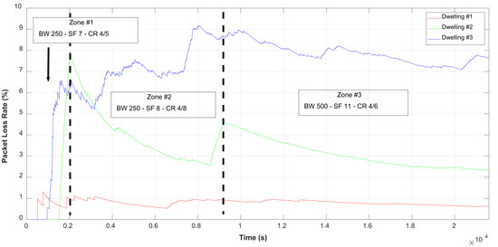
ABC Algorithm Test
5.3. Measurement of Electrical Variables
5.4. Daily Load Profiles
- Analysis and forecast of the demand.
- Adjustment of the electricity bill.
- Power factor improvement.
- Energy efficiency and reduction of electricity consumption.
6. Conclusions
Author Contributions
Funding
Acknowledgments
Conflicts of Interest
Abbreviations
| AMR3 | Arduino Mega R3 |
| AUR3 | Arduino Uno R3 |
| AE | Active energy |
| BW | Bandwidth |
| CF | Carrier Frequency |
| CR | Code Rate |
| D | Number of Random Indexes |
| DLGS | Dragino LoRa Shield |
| EMDD | Energy Measurement Device for Dwelling |
| GLNM | Gateway LoRa Network Monitor |
| IoT | Internet of Things |
| LoRa | Long Range |
| LoRaWAN | Long Range Wide Area Network |
| LPWAN | Low Power Wide Area Network |
| MQTT | Message Queue Telemetry Transport |
| p | Number of possible solutions |
| P | Active power |
| pop | Population |
| PL | PayLoad |
| PLR | Packet Lost Rate |
| RSSI | Received Signal Strength Indicator |
| RMS | Root Means Square |
| SF | Spreading Factor |
| SM | Smart Meter |
| t | Time |
| ToA | Time on Air |
| WNS | Wireless Sensor Networks |
| Greek symbols | |
| µ | mean |
| σ | standard deviation |
| Subscripts | |
| min | minimum |
| max | maximum |
| p | preamble |
| max | maximum possible |
| PHY | symbols transmitted in the physical message |
| pk | packet |
| sym | symbol |
References
- Karaboga, D.; Basturk, B. On the performance of artificial bee colony (ABC) algorithm. Appl. Soft Comput. 2008, 8, 687–697. [Google Scholar] [CrossRef]
- Karaboga, D.; Ozturk, C. A novel clustering approach: Artificial Bee Colony (ABC) algorithm. Appl. Soft Comput. 2011, 11, 652–657. [Google Scholar] [CrossRef]
- Karaboga, D.; Akay, A. A modified Artificial Bee Colony (ABC) algorithm for constrained optimization problems. Appl. Soft Comput. 2011, 11, 3021–3031. [Google Scholar] [CrossRef]
- Cano-Ortega, A.; Sánchez-Sutil, F.J.; Hernández, J.C. Power Factor Compensation using Teaching Learning Based Optimization and Monitoring System by Cloud Data Logger. Sensors 2019, 19, 2172. [Google Scholar] [CrossRef] [Green Version]
- Mohandas, N.; Balamurugan, R.; Lakshminarasimman, L. Optimal location and sizing of real power DG units to improve the voltage stability in the distribution system using ABC algorithm united with chaos. Electr. Power Energy Syst. 2015, 66, 41–52. [Google Scholar] [CrossRef]
- Sen, T.; Datt Mathur, H. A new approach to solve Economic Dispatch problem using a Hybrid ACO–ABC–HS optimization algorithm. Electr. Power Energy Syst. 2016, 78, 735–744. [Google Scholar] [CrossRef]
- Gaidhane, P.J.; Nigam, M.J. A hybrid grey wolf optimizer and artificial bee colony algorithm for enhancing the performance of complex systems. J. Comput. Sci. 2018, 27, 284–302. [Google Scholar] [CrossRef]
- Naidua, K.; Hazlie Mokhlis, H.; Abu Bakar, A.H.; Terzija, V. Performance investigation of ABC algorithm in multi-area power system with multiple interconnected generators. Appl. Soft Comput. 2017, 57, 436–451. [Google Scholar] [CrossRef]
- Juneja, M.; Nagar, S.K.; Mohanty, S.R. ABC based reduced order modelling of microgrid in grid-tied mode. Control Eng. Pract. 2019, 84, 337–348. [Google Scholar] [CrossRef]
- Kumar Paliwal, N.; Kumar Singh, A.; Kumar Singh, N. A day-ahead optimal energy scheduling in a remote microgrid alongwith battery storage system via global best guided ABC algorithm. J. Energy Storage 2019, 25, 100877. [Google Scholar] [CrossRef]
- Ghosh, S.; Karar, V. Assimilation of Optimal Sized Hybrid Photovoltaic-Biomass System by Dragonfly Algorithm with Grid. Energies 2019, 11, 1892. [Google Scholar] [CrossRef] [Green Version]
- Ali Ertürk, M. Lorawan indoor performance analysis. Int. Res. J. Comput. Sci. 2017, 4, 23–29. [Google Scholar] [CrossRef]
- Petajajarvi, J.; Mikhaylov, K.; Pettissalo, M.; Janhunen, J.; Iinatti, J. Performance of a low-power wide-area network based on LoRa technology: Doppler robustness, scalability, and coverage. Int. J. Distrib. Sens. Netw. 2017, 13. [Google Scholar] [CrossRef] [Green Version]
- Yousuf, A.M.; Rochester, E.M.; Ousat, B.; Ghaderi, M. A Throughput, Coverage and Scalability of LoRa LPWAN for Internet of Things. In Proceedings of the 2018 IEEE International Symposium on Quality of Service (IWQoS), Banff, AB, Canada, 4–6 June 2018. [Google Scholar] [CrossRef]
- Hoeller, A., Jr.; Demo Souza, W.; Alcaraz Lopez, R.; Onel, L. Analysis and Performance Optimization of LoRa Networks with Time and Antenna Diversity. IEEE Access 2018, 6, 32820–32829. [Google Scholar] [CrossRef]
- Kerkouche, R.; Alami, R.; Féraud, R.; Varsier, N.; Maillé, P. Node-based optimization of LoRa transmissions with Multi-Armed Bandit algorithms. In Proceedings of the 2018 International Conference on Telecommunications (ICT), St. Malo, France, 26–28 June 2018; pp. 521–526. [Google Scholar]
- Taha, A.A.; Feteiha, M.F.; Abdul, W. Performance Evaluation for LoRa Transceiver. Int. J. Comput. Sci. Softw. Eng. 2019, 8, 25–39. [Google Scholar]
- Sandoval, R.M.; Garcia-Sanchez, A.J.; Garcia-Haro, J. Performance optimization of LoRa nodes for the future smart city/industry. J. Wirel. Commun. Netw. 2019, 2019, 200. [Google Scholar] [CrossRef]
- Cano-Ortega, A.; Sánchez-Sutil, F.J. Monitoring of the Efficiency and Conditions of Induction Motor Operations by Smart Meter Prototype Based on a LoRa Wireless Network. Electronics 2019, 8, 1040. [Google Scholar] [CrossRef] [Green Version]
- Benzi, F.; Anglani, N.; Bassi, E.; Frosini, L. Electricity Smart Meters Interfacing the Dwellings. IEEE Trans. Ind. Electron. 2011, 58, 10. [Google Scholar] [CrossRef]
- Minchala-Avila, L.I.; Armijos, J.; Pesánteza, D.; Zhang, Y. Design and Implementation of a Smart Meter with Demand Response Capabilities. Energy Procedia 2016, 103, 195–200. [Google Scholar] [CrossRef]
- Kumar, A.; Thakur, S.; Bhattacharjee, P. Real time monitoring of AMR enabled energy meter for AMI in Smart City-An IoT Application. In Proceedings of the 2018 IEEE International Symposium on Smart Electronic Systems (iSES), Hyderabad, India, 17–19 December 2018. [Google Scholar]
- Sun, Y.; Lampe, L.; Wong, V.W.S. Smart Meter Privacy: Exploiting the Potential of Dwelling Energy Storage Units. IEEE Internet Things J. 2018, 5, 69–78. [Google Scholar] [CrossRef]
- Sánchez-Sutil, F.; Cano-Ortega, A.; Hernández, J.C.; Rus-Casas, C. Development and calibration of an open source, low-cost power smart meter prototype for PV dwelling-prosumers. Electronics 2019, 8, 878. [Google Scholar] [CrossRef] [Green Version]
- Avancini, D.B.; Rodrigues, J.P.C.; Martins, S.G.B.; Rabêlo, R.A.; Al-Muhtadi, J.; Solic, P. Energy meters evolution in smart grids: A review. J. Clean. Prod. 2019, 217, 702–715. [Google Scholar] [CrossRef]
- Stegner, C.; Oliver Glaß, O.; Beikircher, T. Comparing smart metered, residential power demand with standard load profiles. Sustain. Energy Grids Netw. 2019, 20, 100248. [Google Scholar] [CrossRef]
- Akselrad, D.; Petcu, V.; Römer, B.; Schmid, A.; Bytschkow, D.; Engelken, M. Making Home Energy Usage Transparent for Dwellings using Smart Meters. In Proceedings of the 2011 IEEE International Conference on Consumer Electronics, Berlin, Germany, 6–8 September 2011. [Google Scholar]
- Haben, S.; Singleton, C.; Grindrod, P. Analysis and Clustering of Residential Customer Energy Behavioral Demand Using Smart Meter Data. IEEE Trans. Smart Grid 2016, 7, 136–144. [Google Scholar] [CrossRef]
- Wesley Schultz, P.; Mica Estrada, M.; Schmitt, J.; Sokoloski, R.; Silva-Send, N. Using in-home displays to provide smart meter feedback about dwelling electricity consumption: A randomized control trial comparing kilowatts, cost, and social norms. Energy 2015, 90, 351–358. [Google Scholar] [CrossRef] [Green Version]
- Anderson, B.; Lin, S.; Newing, A.; Bahaj, A.; James, P. Electricity consumption and dwelling characteristics: Implications for census-taking in a smart metered future. Comput. Environ. Urban Syst. 2017, 63, 58–67. [Google Scholar] [CrossRef] [Green Version]
- Gouveia, J.P.; Júlia Seixas, J.; Mestre, A. Daily electricity consumption profiles from smart meters - Proxies of behavior for space heating and cooling. Energy 2017, 141, 108–122. [Google Scholar] [CrossRef]
- Dudek, G.; Gawlak, A.; Kornatka, M. Analysis of Smart Meter Data for Electricity Consumers. In Proceedings of the 2018 International Conference on the European Energy Market (EEM), Lodz, Poland, 27–29 June 2018. [Google Scholar]
- Funde, N.; Dhabu, M.; Balande, U. Motif-based Pattern Detection Method for Smart Energy Meter Data. In Proceedings of the 2018 IEEE International Conference for Convergence in Technology, Pune, India, 6–8 April 2018. [Google Scholar]
- Nilsson, A.; Wester, M.; David Lazarevic, D.; Brandt, N. Smart homes, home energy management systems and real-time feedback: Lessons for influencing dwelling energy consumption from a Swedish field study. Energy Build. 2018, 179, 15–25. [Google Scholar] [CrossRef]
- Yildiz, B.; Bilbao, J.I.; Dore, J.; Sproul, A. Dwelling electricity load forecasting using historical smart meter data with clustering and classification techniques. In Proceedings of the 2018 IEEE Innovative Smart Grid Technologies—Asia (ISGT Asia), Singapore, 22–25 May 2018. [Google Scholar]
- Laicane, I.; Blumberga, A.; Rosa, M.; Blumberga, D. The Effect of the Flows of Information on Residential Electricity Consumption: Feasibility Study of Smart Metering Pilot in Latvia. In Proceedings of the European Conference on Smart Objects, Systems and Technologies, Erlangen/Nuremberg, Germany, 11–12 June 2013. [Google Scholar]
- Rahman, M.; Alfaki, A.; Shafiullah, G.M.; Shoeb, A.; Jamal, T. Demand Response Opportunities in Residential Sector Incorporated with Smart Load Monitoring System. In Proceedings of the 2016 IEEE Innovative Smart Grid Technologies, Melbourne, VIC, Australia, 28 November–1 December 2016. [Google Scholar]
- Sial, A.; Singh, A.; Mahanti, A. Detecting anomalous energy consumption using contextual analysis of smart meter data. Wirel. Netw. 2019. [Google Scholar] [CrossRef]
- Sial, A.; Singh, A.; Mahanti, A.; Gong, M. Heuristics-Based Detection of Abnormal Energy Consumption. In Smart Grid and Innovative Frontiers in Telecommunications; Springer: Auckland, New Zealand, 2018; pp. 21–31. [Google Scholar]
- Sial, A.; Singh, A.; Mahanti, A.; Gong, M. Profiling Energy Consumption in a Residential Campus. In Proceedings of the 2014 CoNEXT on Student Workshop, Sydney, Australia, 2–5 December 2014; pp. 15–17. [Google Scholar] [CrossRef] [Green Version]
- Sánchez-Sutil, F.; Cano-Ortega, A. Smart public lighting control and measurement system using LoRa network. Electronics 2020, 9, 124. [Google Scholar] [CrossRef] [Green Version]
- Noreen, U.; Bounceur, A.; Clavier, L. A Study of LoRa Low Power and Wide Area Network Technology. In Proceedings of the 2017 International Conference on Advanced Technologies for Signal and Image Processing (ATSIP), Fez, Morocco, 22–24 May 2017. [Google Scholar] [CrossRef]
- Phung, K.H.; Hieu Tran, H.; Nguyen, Q.; Huong, T.T.; Nguyen, T.L. Analysis and Assessment of LoRaWAN. In Proceedings of the 2018 2nd International Conference on Recent Advances in Signal Processing. Telecommunications & Computing (SigTelCom), Ho Chi Minh City, Vietnam, 29–31 January 2018. [Google Scholar] [CrossRef]
- Bouguera, T.; Diouris, J.F.; Chaillout, J.J.; Jaouadi, R.; Andrieux, G. Energy Consumption Model for Sensor Nodes Based on LoRa and LoRaWAN. Sensors 2018, 18, 2104. [Google Scholar] [CrossRef] [PubMed] [Green Version]
- Polonelli, T.; Brunelli, D.; Marzocchi, A.; Benini, L. Slotted ALOHA on LoRaWAN-Design, Analysis, and Deployment. Sensors 2019, 19, 838. [Google Scholar] [CrossRef] [PubMed] [Green Version]
- Sornin, N.; Yegin, A. LoRaWANTM 1.1 Specification. 2017. Available online: https://lora-alliance.org/sites/default/files/2018-04/lorawantm_specification_-v1.1.pdf (accessed on 10 December 2019).
- LoRa Alliance Technical Committee Regional Parameters Workgroup. LoRaWANTM 1.1 Regional Parameters. 2018. Available online: https://lora-alliance.org/sites/default/files/2018-04/lorawantm_regional_parameters_v1.1rb_-_final.pdf (accessed on 10 December 2019).
- Arduino Mega Rev3. Available online: https://store.arduino.cc/mega-2560-r3 (accessed on 10 December 2019).
- Dragino LoRa GPS Shield for Arduino. Available online: https://www.dragino.com/products/lora/item/108-lora-gps-shield.html (accessed on 10 December 2019).
- Ningbo Peacefair Electronic Co., Ltd. Available online: https://peacefair.en.made-in-china.com (accessed on 10 December 2019).
- Wemos Electronics. Available online: https://wiki.wemos.cc/products:d1:d1_mini_pro (accessed on 10 December 2019).
- Firebase. Available online: https://www.firebase.google.com (accessed on 10 December 2019).
- Arduino MKR WAN 1300. Available online: https://store.arduino.cc/mkr-wan-1300 (accessed on 10 December 2019).
- Monteino. Available online: https://lowpowerlab.com/guide/moteino/ (accessed on 10 December 2019).
- Lopy4. Available online: https://docs.pycom.io/gettingstarted/connection/lopy4/ (accessed on 10 December 2019).
- Libelium. Available online: http://www.libelium.com/extreme-range-wireless-sensors-connectivity-through-buildings-in-city-lora-868mhz-915mhz/ (accessed on 22 November 2019).
- Dragino LoRa Products. Available online: http://www.dragino.com/products/lora.html (accessed on 10 December 2019).
- Murata Electronics. Available online: https://wireless.murata.com/pub/RFM/data/type_abz.pdf (accessed on 10 December 2019).
- HOPERF chip RFM95/96/97/98. Available online: https://cdn.sparkfun.com/assets/learn_tutorials/8/0/4/RFM95_96_97_98W.pdf (accessed on 10 December 2019).
- Semtech SX1276/SX1278 LoRa Chip. Available online: https://www.semtech.com/products/wireless-rf/lora-transceivers/sx1276 (accessed on 10 December 2019).
- Semtech SX1272 LoRa Chip. Available online: https://www.semtech.com/products/wireless-rf/lora-transceivers/sx1272 (accessed on 10 December 2019).
- FZ0430 Voltage Sensor. Available online: http://www.ekt2.com/pdf/412_ARDUINO_SENSOR_VOLTAGE_DETECTOR.pdf (accessed on 10 December 2019).
- ZMPT101B Voltage Sensor. Available online: https://www.datasheet4u.com/datasheet-742pdf/ETC/ZMPT101B/pdf.php?id=1031464 (accessed on 10 December 2019).
- ACS712. Available online: https://www.sparkfun.com/datasheets/BreakoutBoards/0712.pdf (accessed on 10 December 2019).
- STC013 Dechang Electronics Co. Ltd. Available online: http://en.yhdc.com/product/SCT013-401.html.737 (accessed on 10 December 2019).


| Bibliography | Parameters Measured | Features | Topics |
|---|---|---|---|
| [20] | --- | Study of SMs international regulation | Local interface of SMs in households |
| [21] | Voltage and current | SM Design | Demand response capabilities |
| [22] | Energy consumption | LDR to measure SMs pulses | Monitoring electrical energy consumption |
| [23] | Electricity consumption | Thermal and chemical energy storage Electric vehicles | System model Optimization of energy storage units |
| [24] | Voltage, current and active power | Cloud computing storage High accuracy | Development, calibration and uncertainty studies of SM |
| [25] | --- | Energy meters evolution in smart grids | Types of SMs (precise measuring, data storage, communication networks, home control, system security) |
| [26] | Voltage, current, PF | Measure time 15 s Results analysis and validation | Comparison of standard load profiles with those obtained with SMs |
| [27] | Power consumption | Optical sensor to SMs | Analysis of measured data to improve electrical energy consumption |
| [28] | Energy consumption | Commercial SMs | Data analysis and clustering |
| [29] | Energy consumption | ZigBee wireless | Data analysis in different scenarios |
| [30] | Energy consumption | Commercial SMs | study and estimation of indicators of load profiles in dwellings |
| [31] | Energy consumption | Commercial SMs Measure time 15 min | Obtaining and analysis of load profiles in houses in Evora (Portugal) |
| [32] | Energy consumption | Commercial SMs Measure time 15 min | Obtaining and analysis of load profiles in 1000 houses in Poland |
| [33] | Energy consumption | Commercial SMs Measure time 30 min | Smart meter dataset Data Analysis and Clustering |
| [34] | Energy consumption | Commercial SMs | Obtaining and analysis of load profiles in 154 houses in Stockholm (Sweden) |
| [35] | Energy consumption | Commercial SMs | Data analysis and Clustering |
| [36] | Energy consumption | Commercial SMs | Obtaining and analysis of load profiles in 1000 houses in Latvia |
| [37] | Voltage, current and active power | Power Tracker SM Measure time 60 s ZigBee Wireless | Monitoring the electricity consumption of domestic appliances in an Australian house |
| [38,39] | Electrical variables | Schneider Electric EM64XX | Application of heuristic techniques for the detection of abnormal energy consumption |
| [40] | Electrical variables | Schneider Electric EM64XX | Classification of load profiles |
| [41] | Voltage, current, active power and illumination level | Control and measurement system design LoRa wireless Measure time 5 s | Smart public Lighting control Energy efficiency |
| Description | Number | Total Price (€) |
|---|---|---|
| Microcontroller AMR3 | 1 | 28.00 |
| Lora GPS shield DLGS | 1 | 35.90 |
| PZEM-004t | 1 | 10.08 |
| Box container | 1 | 6.98 |
| AC/DC power supply adapter | 1 | 1.87 |
| Auxiliary material and wiring | 1 | 3.58 |
| Total cost | 86.41 |
| Description | Number | Total Price (€) |
|---|---|---|
| Microcontroller AMR3 | 1 | 28.00 |
| Lora GPS shield DLGS | 1 | 35.90 |
| Microcontroller WMP | 1 | 4.61 |
| Box container | 1 | 6.98 |
| AC/DC power supply adapter | 1 | 1.87 |
| Auxiliary material and wiring | 1 | 2.47 |
| Total cost | 79.83 |
| Dwelling | Type | Surface Area (m2) | Distance to GLNM (km) |
|---|---|---|---|
| #1 | Flat | 65 | 1.663 |
| #2 | Town home | 160 | 1.046 |
| #3 | Single-family home | 320 | 0.923 |
| Device | Place | UTM Coordinates Zone 30 | |
|---|---|---|---|
| X (m) | Y (m) | ||
| EMDD #1 | Dwelling #1 | 430,235 | 4,181,413 |
| EMDD #2 | Dwelling #2 | 430,449 | 4,182,444 |
| EMDD #3 | Dwelling #3 | 430,596 | 4,182,314 |
| Gateway | Terrace of Higher Polytechnic School of Jaen | 431,502 | 4,182,490 |
| BW (kHz) | RSSI (dBm) | PLR (%) | ||
|---|---|---|---|---|
| μ | σ | μ | σ | |
| 125 | −93.4514 | 12.4805 | 35.4514 | 46.7468 |
| 250 | −94.0305 | 8.1476 | 17.9331 | 37.5216 |
| 500 | −91.7110 | 2.5139 | 1.1024 | 1.1724 |
| BW (kHz) | SF | CR | ||||||||
|---|---|---|---|---|---|---|---|---|---|---|
| 7 | 8 | 9 | 10 | 11 | 12 | 4/5 | 4/6 | 4/7 | 4/8 | |
| 125 | −99.904 | −101.098 | −101.704 | −103.696 | −76.000 | −76.000 | −93.111 | −93.795 | −91.254 | −94.102 |
| 250 | −97.221 | −98.090 | −97.581 | −97.801 | −96.988 | −76.500 | −92.566 | −94.606 | −94.848 | −94.102 |
| 500 | −92.357 | −92.202 | −92.375 | −92.337 | −91.046 | −89.947 | −94.934 | −90.478 | −90.749 | −90.683 |
| BW (kHz) | RSSI (dBm) | PLR (%) | ||
|---|---|---|---|---|
| μ | σ | μ | σ | |
| 125 | −84.3133 | 6.4948 | 34.7193 | 47.2516 |
| 250 | −84.1053 | 4.0593 | 17.1566 | 37.8496 |
| 500 | −91.4427 | 4.6983 | 3.2301 | 7.7366 |
| BW (kHz) | SF | CR | ||||||||
|---|---|---|---|---|---|---|---|---|---|---|
| 7 | 8 | 9 | 10 | 11 | 12 | 4/5 | 4/6 | 4/7 | 4/8 | |
| 125 | −88.615 | −87.946 | −87.168 | −90.149 | −76.000 | −76.000 | −84.833 | −85.252 | −82.961 | −84.206 |
| 250 | −85.214 | −86.777 | −84.019 | −84.918 | −85.197 | −76.500 | −83.786 | −84.889 | −83.971 | −83.775 |
| 500 | −91.491 | −91.872 | −91.152 | −91.143 | −90.597 | −92.401 | −92.749 | −92.556 | −96.283 | −84.181 |
| BW (kHz) | RSSI (dBm) | PLR (%) | ||
|---|---|---|---|---|
| μ | σ | μ | σ | |
| 125 | −97.2245 | 15.5412 | 39.2390 | 47.6840 |
| 250 | −15.7636 | 13.6237 | 18.7191 | 37.1631 |
| 500 | −111.3174 | 4.1290 | 11.3068 | 5.8131 |
| BW (kHz) | SF | CR | ||||||||
|---|---|---|---|---|---|---|---|---|---|---|
| 7 | 8 | 9 | 10 | 11 | 12 | 4/5 | 4/6 | 4/7 | 4/8 | |
| 125 | −107.939 | −107.479 | −108.538 | −107.389 | −76.000 | −76.000 | −97.917 | −98.954 | −96.698 | −98.327 |
| 250 | −111.110 | −110.820 | −111.654 | −113.007 | −111.490 | −76.500 | −102.972 | −105.376 | −107.585 | −107.121 |
| 500 | −109.233 | −109.464 | −110.686 | −112.776 | −112.773 | −113.972 | −107.612 | −113.520 | −113.589 | −110.548 |
© 2020 by the authors. Licensee MDPI, Basel, Switzerland. This article is an open access article distributed under the terms and conditions of the Creative Commons Attribution (CC BY) license (http://creativecommons.org/licenses/by/4.0/).
Share and Cite
Cano-Ortega, A.; Sánchez-Sutil, F. Performance Optimization LoRa Network by Artificial Bee Colony Algorithm to Determination of the Load Profiles in Dwellings. Energies 2020, 13, 517. https://doi.org/10.3390/en13030517
Cano-Ortega A, Sánchez-Sutil F. Performance Optimization LoRa Network by Artificial Bee Colony Algorithm to Determination of the Load Profiles in Dwellings. Energies. 2020; 13(3):517. https://doi.org/10.3390/en13030517
Chicago/Turabian StyleCano-Ortega, A., and F. Sánchez-Sutil. 2020. "Performance Optimization LoRa Network by Artificial Bee Colony Algorithm to Determination of the Load Profiles in Dwellings" Energies 13, no. 3: 517. https://doi.org/10.3390/en13030517