Global Horizontal Irradiance Modeling for All Sky Conditions Using an Image-Pixel Approach

Abstract

Ground images with a sky camera have become common to evaluate cloud coverage, aerosols, and energy collection. In parallel, the growth of solar energy has led to an impulse to evaluate and forecast the solar potential in a site before investments, which has increased the importance of solar power measurements. Facing that scenario, this work presents a novel sky camera model that allows to measure the global horizontal irradiance (GHI). Initially, images from a fisheye camera were stored and a pixel-based approach model was created for cloud segmentation. A total of 813 k vectors of features were used as input to the support vector machine for classification (SVC), which yielded a success rate of about 98.6% in accuracy. The Sun’s position was also segmented and an artificial neural network (ANN) regression model for GHI with 17 input features was created based on segmentation of the Sun, clouds, and sky. The training/validation stage of the ANN used 89,964 samples and the test stage reached about 97.4% in Pearson’s correlation. The RMSE was 72.3 W/m² for GHI and the normalized RMSE, nRMSE, revealed 12.9% for GHI. That nRMSE value was comparable to or lower than other studies, despite the high fluctuations in the observed GHI.

1. Introduction

The expressive growth of solar energy has been followed by much research on how to efficiently prospect this type of energy. As a result, new methods for assessing solar resources have been developed with improvements in the techniques used so far. They have played an important role in reducing the risk in choosing a location for a power plant. Other goals have been targeted as the selection of the source of solar energy generation and the design of the appropriate energy conversion technology to be deployed [1]. In this scenario, the clouds deserve special attention, given that they are responsible for blocking the incoming Sun radiation. They can drastically reduce the amount of energy that reaches the collectors in a plant. Cloud displacement is also the cause of significant fluctuations in solar power generation [2].

The ability to predict the energy production in a site has become fundamental in the development of solutions to deliver electrical power as stably as possible to the distribution network [3]. Once that the energy average production estimate is acquired by power plants in reliable long-, medium-, or short-term data, strategies of generation can be planned. Therefore, gathering information with respect to atmospheric conditions is one of the main requirements for solar power plants to improve system performance, allowing plant operators to adapt their plant’s operation modes to the meteorological conditions [4]. It can be said that adequate solar irradiance forecasting is an important tool to help the grid operators to optimize their electricity production and to reduce additional costs by preparing an appropriate strategy [5], which will impact the total energy generation cost.

The global horizontal irradiance, or GHI, is the standard measure of total available solar radiation, typically measured using a thermopile or photodiode pyranometer. In the assessment of the potential of solar energy in a site, the GHI measurements play an important source of information amid other solar radiation parameters [6]. It must be noted that measurements of GHI made with high-quality and well-maintained instruments have 95% confidence intervals around ±3% to ±10%, depending on the solar zenith angle [7]. Accuracy is normally related to cost, so it is worth noting that properly calibrated and well-maintained sensors have a high cost.

Despite solar irradiance sensors remaining widely used to obtain GHI, another type of equipment, i.e., sky imaging system, has been frequently used for solar and atmospheric research and applications: aerosol characterization, cloud detection and tracking [8], automatic cloud coverage computation, cloud-base height estimation, and solar forecasting. They capture hemispherical images of the sky at regular intervals using a fish-eye lens. The accurate estimation of solar irradiance using exclusively those images is, therefore, also a first step towards the short-term forecasting of solar energy generation based on cloud movement.

Commercial sky imaging devices are now becoming common [9]. Indeed, some brands like the Whole Sky Imager systems (WSI), using digital imaging technology, were deployed since the early 1980s [10]. However, traditional brands of sky imagers include complex, not totally robust, and costly mechanical systems of shadow bands designed to avoid the direct radiation beam over the image sensor. On the other hand, instead of acquiring traditional brands of sky imagers, there is an option of achieving images from fish-eye cameras deployed as a ground-based imagery system [11].

At the time this text is being written, there are not many articles in the literature about modeling GHI from a sky camera. Kurtz managed to model irradiances by using an artificial neural network (ANN) to achieve some results in light of the image sensor charge couple device (CCD) smear that results from the presence of a very bright light sources such as the Sun [7]. That approach relies on methods to calibrate irradiance based on measuring the direct normal irradiance (DNI) using CCD smear with a UCSD Sky Imager. About the method, the authors admitted the need to improve the procedures for DNI calibration, particularly with respect to detection of clear-sky periods. That work obtained a nRMSE of 9–11% for GHI. Gauchet, by its time, developed a method based on radiation transfer functions and cloud segmentation using a low-cost fish-eye camera [12]. The nRMSE was 17% regarding 5 min averaging data. The research developed by Schmidt was based on machine learning algorithms with image features and irradiance measurements [13]. In order to acquire images, a low-cost fish-eye camera Vivotec used in closed-circuit TV (CCTV) was deployed. A total of 37 possible features were used with models based on the k-nearest-neighbor (KNN) classifier machine learning algorithm to estimate internal parameters. The study managed to estimate GHI with a nRMSE of 26.6% and correlation of 94.1%.

Within that scenario and knowing that the GHI is an essential parameter in solar resource assessment, this work presents a novel algorithm to model that parameter from images based on a low cost, 180° aperture, fish-eye camera that can be found on the shelves. The present work was based on two models in a cascading scheme. The first one is for cloud segmentation in an image through the use of a machine learning and added to the segmentation of the Sun disk, both for pixel classification. The second model is for regression in order to estimate the GHI. Both model conceptions required the development of new classification and regression features not found in other works. It is important to mention that the study was carried out in a coastal zone, characterized by having a tropical climate and expressive irradiance variability.

2. Feature Review in Cloud Segmentation

The segmentation of clouds within images is a fundamental step in developing this research. As an image contains sets of points making part of objects or shapes, each point, or pixel, in the image can be represented by means of the color space known as RGB, in which R stands for the red color channel intensity, G for the green color channel intensity, and B for the blue color channel intensity, all of them integer numbers varying between 0 to 255, due to a resolution of 8 bits per channel. For the purpose of cloud segmentation, so many papers in the literature have explored the importance of the R/B ratio to segment clouds in images. That is the case of the work of Chow [14], who also used threshold values for the construction of a decision algorithm to detect cloud pixels. The average value of R/B was implemented as a classification parameter as it is used to identify whether there is Sun shadowing. In other work, Chow used a camera with 12 bits of resolution in each RGB channel [15], so that the R/B feature was also included in their research due to the segmentation properties it offers. The usefulness of this feature is corroborated by the work of Fu [16]. According to them, this quotient is typically used to determine if the dominant source of the pixel represents clear sky or clouds.

Liu [17], on the other hand, developed a cloud detection method based on an algorithm named “superpixel segmentation (SPS)” [18], a popular technique already used in the field of image segmentation. The name of the algorithm is due to the fact that the image is divided in irregular regions denominated “superpixels”. This irregular division is based on texture similarities, brightness similarities, and contour continuity in an image. For each image region, or superpixel, a threshold is obtained. Considering all regions, a threshold matrix is created through bilinear interpolation of local thresholds. Finally, the detection of clouds is achieved with pixel-to-pixel comparison between a feature derived from the expression (R − B) and the threshold matrix. The results presented accuracy, F-Score, precision, and recall, above 82%, 84%, and 81%, respectively, for one database and 93%, 94%, and 92%, respectively, for another database. Cloud segmentation in night images have also used the superpixel concept [19], as well as parameters that are usual in the daytime segmentation.

Narain’s article brought a compilation of 10 algorithms developed for cloud segmentation [20]. The simplest algorithm used pre-established thresholds based on the R/B and (R − B) features for segmentation. Another algorithm used a more sophisticated method through the fast Fourier transform (FFT) method to analyze the homogeneity of symmetrical pixels of an image, knowing that in the absence of clouds there is a greater homogeneity in the color elements of the sky under analysis. Then, comparisons based on B/R ratio and histograms relative to that parameter are performed. In the final step, there is a search mechanism for cloud contours. Other methods mentioned in that compilation used the (B − R)/(B + R) ratio, the k-means clustering, or the fuzzy clustering neural networks as classification mechanisms. The last method mentioned, denominated “graph cut algorithm”, reached an accuracy of 94.7% in the classification. It should be noted that other works, such as that of Marquez [21], also used the (B − R)/(B + R) feature as a normalized alternative for the R/B feature.

Dev’s study [22], by its time, worked on cloud segmentation from the perspective of bimodality [23]. In that case, applied to the distribution of parameters based on color spaces. The analysis based on PCA, principal component analysis, was also part of that work. Subsequently, a tool for pixel classification was applied using the fuzzy clustering artificial neural network. Various color spaces were analyzed in the search for the best parameters that produced bimodal distributions through their components: red-green-blue (RGB), Hue-Saturation-Value (HSV), luma-chrominance-chrominance (YIQ), luminance-color-color (CIE) and luminance-color-color components (Lab). From these color spaces, the authors selected three parameters as the most important from the bimodality point of view (S; R/B; and (B − R)/(B + R)). The evaluation using the principal component analysis (PCA) method also evidenced these same three parameters for their significance. A posterior evaluation regarding a two dimensional approach indicated that the difference between the component I (from the color space YIQ) and the three previous components resulted in three even more significant components, i.e., S − I; R/B − I; and (B − R)/(B + R) − I. The last algorithm led to an increase in precision, initially at 84%, to around 90%.

Chu proposed the R/B, (B − R) and (B − R)/(B + R) features [24], said to be widely used to identify the presence of clouds. According to that work, (B − R)/(B + R) is considered an improvement in terms of robustness, because it avoids extremely high (R/B) values when the pixels have very low B channel values.

As seen in some papers [25,26], the deployment of masks in sky images are useful, since they eliminate objects that are not part of the study, simplifying it. Chu [26], for instance, developed an algorithm that was created to apply an automatic mask with the purpose of separating the sky area from ground obstacles and image edges for each image collected.

3. Materials and Methods

3.1. Equipment

For the purpose of the experiment, the images were captured from a camera placed in the laboratory’s roof due to the simplicity of installation and proximity to computers connected to the internet. A video surveillance camera (CCTV) was then selected by its specifications as well as the availability and cost. The camera model adopted was the FE8174V model, with fish-eye type lens (180°), 8-bit resolution per RGB channel, and manufactured by Vivotek (Taipei, Taiwan).

The GHI measurements of GHI and DNI irradiances were performed with the support of a pyranometer and a pyrheliometer. The first and second class of such equipment, according to the ISO 9060 pyranometer specifications, have a maximum uncertainty in measurements of ±20 W/m², while in the secondary standard, the uncertainty is of ±10 W/m². The pyranometer used in this research, model CP-21, made by Kipp & Zonnen (Delft, The Netherlands), has an accuracy of ±10 W/m², and the pyrheliometer, model sNIP, made by Eppley Laboratory, Inc. (Newport, USA), has an accuracy of ±10 W/m².

3.2. Cloud Segmentation

After the development of a C# software to capture and store images, sequences of photographs were recorded throughout the day in 5 s intervals for post-processing with a resolution of 1056 × 1056 pixels. Subsequently, both horizontal and vertical sizes of pictures were reduced to 528 × 528, because it was verified that there was no loss in cloud pixel recognition. In addition, the gain in image processing time was quite evident with this reduction in size. It is worth saying that some resources of the camera, like Back Light Compensation (BLC) and Wide Dynamic Range (WDR), were disabled to get raw images.

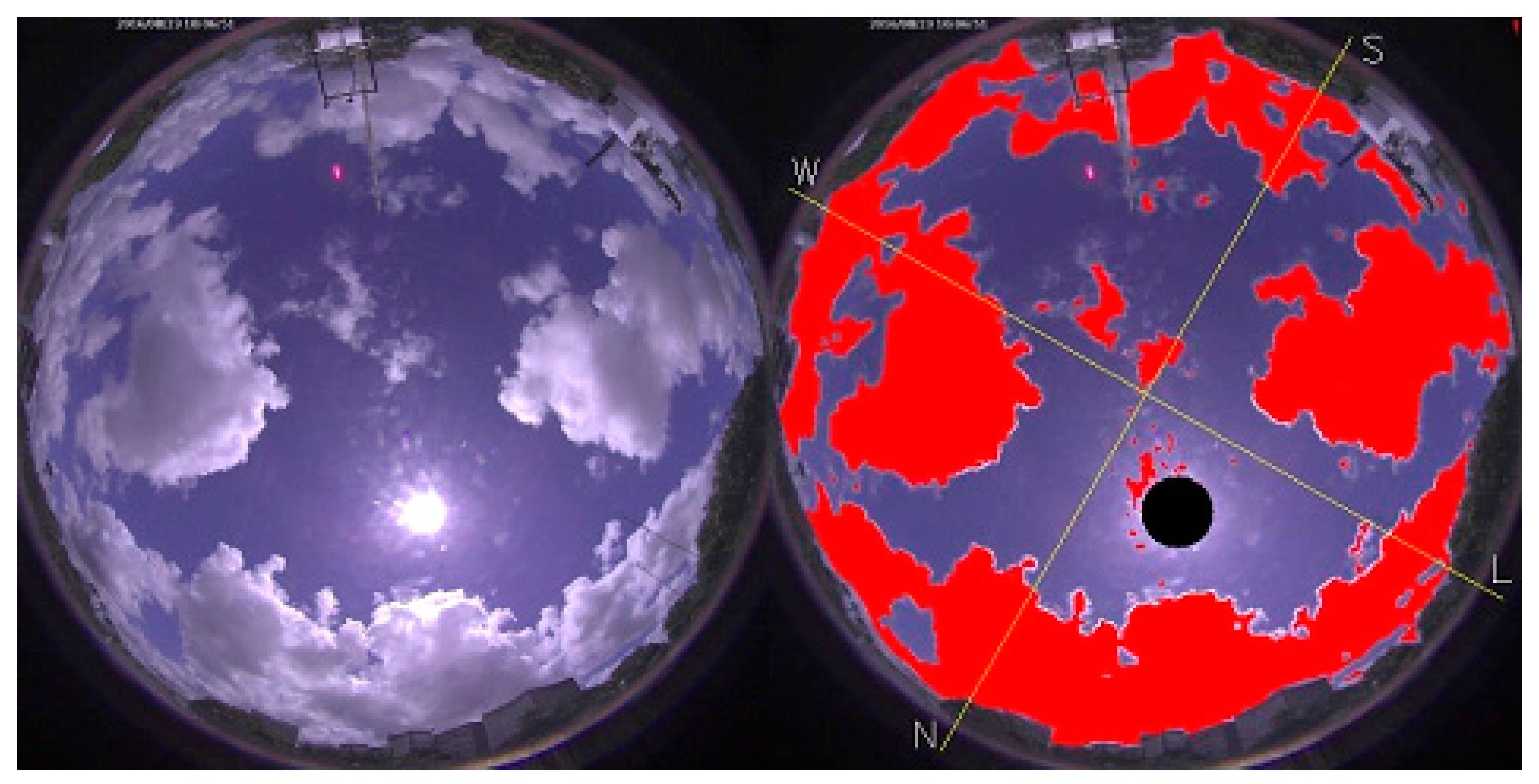
After the image dataset was created, the next step was to manually label clouds by painting the regions of interest (ROI) in a subset of images to use as inputs to a model. Indeed, labeling the pixels manually is a procedure required by a SVC-supervised machine learning algorithm, given that the user needs to teach the algorithm to classify according to what is stated as correct. As an example, in Figure 1, pixels of clouds and sky were labeled with red and black colors, respectively. Images in different hours of the day were used in that labeling scheme. This way, a set of vectors with features could be formed by associating the output of each ROI to a cloud (1-value) or sky (0-value).

To automatically classify pixels as cloud or sky, a search was performed to find features or attributes to be used as inputs in a support vector machine (SVM, or SVC for classification), a type of machine learning (ML) algorithm. The chosen features were created by what is called “feature engineering” or selected from those features showed in the papers mentioned in the Section 2. While being created, all the features were compared with their predecessors in the previous stage to select the best ones according to the following (three) metrics: the Pearson correlation coefficient, Equation (1); the gain rate, Equation (2); and the symmetric uncertainty, Equation (3). The Pearson correlation coefficient or Pearson product-moment correlation coefficient (PPMCC) is a widely used statistic that measures linear correlation between two variables, X and Y. It has a value between +1 and −1. A value of +1 means total positive linear correlation, 0 that is no linear correlation, and −1 means total negative linear correlation. The gain rate, Equation (2), evaluates the value of an attribute by measuring the rate of gain in relation to the class [27]. The symmetric uncertainty, Equation (3), assesses the value of an attribute by measuring symmetric uncertainty in relation to the class [27]. Both the gain ratio attribute and the symmetric uncertainty attribute are based on the definition of entropy, H (X), and conditional entropy, H (Y|X), Equations (4) and (5), respectively. It is important to note that the dichotomous output variable Y assumes the value of 1 or 0 whether a cloud pixel exists or not. For that reason, mathematically the Pearson correlation coefficient is equivalent to the point-biserial correlation coefficient as a measure of association between a dichotomous variable and a continuous variable [28].

$$r_{X,Y}=\frac{Cov\left(X,Y\right)}{{\sigma }_X{\sigma }_Y}$$

(1)

$$Ginfo(Classe,Atributo=H\left(Classe\right)-H(Classe|Atributo)$$

(2)

$$RGinfo(Classe,Atributo=\frac{H\left(Classe\right)-H(Classe|Atributo)}{H\left(Atributo\right)}$$

(3)

$$H\left(X\right)=- {\displaystyle \sum }_{x \in X}^{}p\left(x\right).log\left(p\left(x\right)\right)$$

(4)

$$H\left(Y|X\right)= - {\displaystyle \sum }_{x \in X}^{}p\left(x\right){\displaystyle \sum }_{y \in Y}^{}p\left(y|x\right).log\left(p\left(y|x\right)\right)$$

(5)

The expressions, from f0 to f6, Equations (6)–(12), were the features obtained in order to improve the classification between clouds and sky regarding the three metrics presented. Here, four color spaces, RGB, HSV, YCrCb, and Lab (or CIELAB), were deployed through their channels. The features $f_0$ and $f_1$ were calculated on the output of an image sent to a CLAHE (contrast limited adaptative histogram equalization) filter [29]. In that case, the CLAHE filter was applied only on the V (brightness) channel of the HSV space.

$$f_0=\frac{\left(Cb1-G1\right)}{\left(Cr1+G1+0.5\right)}-\frac{\left(Cr1-Cb1\right)}{\left(Cr1+Cb1+0.5\right)}$$

(6)

$$f_1=e^{\left[\frac{\left(Cb1-R1\right)}{\left(Cr1+B1+0.5\right)}+e^{\frac{\left(Cb1-a1\right)}{\left(Cr1+R1+0.5\right)}}\right]}$$

(7)

$$f_2=\mathrm{DistanceEuclid}\left(\mathrm{PtSun}\left({\mathrm{x}}_{\mathrm{s}};{\mathrm{y}}_{\mathrm{s}}\right),\mathrm{PtPixel}\left(x;y\right)\right)$$

(8)

$$f_3=\frac{\left(\mathrm{Cb}-\mathrm{G}\right)}{\left(\mathrm{Cr}+\mathrm{G}+0.5\right)}-\frac{\left(\mathrm{Cr}-\mathrm{Cb}\right)}{\left(\mathrm{Cr}+\mathrm{Cb}+0.5\right)}$$

(9)

$$f_4=\frac{\left(\mathrm{Cb}-\mathrm{G}\right)}{\left(\mathrm{Cr}+0.5\right)}-\frac{\left(\mathrm{Cr}-\mathrm{Cb}\right)}{\left(\mathrm{G}+0.5\right)}$$

(10)

$$f_5={\mathrm{e}}^{\left[\frac{\left(\mathrm{Cb}-\mathrm{R}\right)}{\left(\mathrm{Cr}+\mathrm{B}+0.5\right)}+{\mathrm{e}}^{\frac{\left(\mathrm{Cb}-\mathrm{a}\right)}{\left(\mathrm{Cr}+\mathrm{R}+0.5\right)}}\right]}$$

(11)

$$f_6=\mathrm{S}$$

(12)

In which:

• The variables “R”, “B” and “G” come from the color space RGB;
• The variables “Cr” and “Cb” come from the color space YCrCb;
• The variable “a” is a channel in the color space Lab;
• The variables “S” is a channel in the color space HSV;
• The feature “$f_2$”is the distance from the pixel to the center of solar disk;
• The index “1” in the channels inside the “$f_0$” and “$f_1$” feature expressions, like “$G1$”, means that the CLAHE filter was applied.

Approximately 813 k vectors of unique feature coordinates were stored to train and validate the SVC machine learning model.

Table 1. Results of the metrics applied on the features.

Feature	Pearson	Ginfo	RGinfo
$f_0$	0.864	0.771	0.147
$f_1$	0.877	0.745	0.145
$f_2$	0.151	0.043	0.010
$f_3$	0.851	0.792	0.123
$f_4$	0.867	0.795	0.124
$f_5$	0.864	0.764	0.124
$f_6$	0.908	0.756	0.203

shows the results for each metric applied to the features. Despite the feature $f_2$ showing low values for each metric, it was included because it helped the SVC to reach better results. Actually, all features were also evaluated based on the results of the SVC model, so that the best set was being selected.

Keeping in mind histograms, the idea behind each feature is dividing the samples as much as possible into regions (bins) with only cloud or sky dots. Figure 2 shows histograms of the $f_4$ and $f_6$ features, in which the blue dots are representative of clouds and red dots means sky. The separation achieved between cloud and sky pixels can be perceived by taking into account the bins in such histograms where each bin has, in majority, blue or red colors.

The library called LibSVM [30], widely used, was deployed to segment the clouds.

Table 2. Results of training, validation, and testing.

Parameter Evaluated with LibSVM	Score (%)
Cross validation accuracy	98.6
Test accuracy	98.6
F Score	99.0
Precision	98.4
Recall	99.7

shows a synthesis of the results of a training-validation (70%) and test (30%) modeling scheme, regarding a total of 813 thousand vectors.

In Figure 3, there is an example of a cloud segmentation (right) from the previous image (left). The cloud was painted red. The Sun was also segmented in black inside the image, which will be covered in the next topic.

3.3. Sun Segmentation

In order to segment the Sun, it is necessary to know its position in an image. A dioptric omnidirectional camera, which is the case of fish-eye lenses in the camera used, has typical distortions of a barrel shape, Figure 4. Therefore, the correction of distortions is essential to locate the point in the center of solar disk. To accomplish this task, the open source OpenCV library [31] has the implementation of an undistortion algorithm developed by Zhang and Bouguet [32,33]. That algorithm requires calibrating the camera by retrieving the intrinsic parameters. This is done by capturing several images of a chessboard, at a specific standard size, and using such images as inputs for the undistorting algorithm.

Then, a subset of 20 chessboard images, considering a total of 266 images, was selected based on the mean squared error (MSE) metric, which is the output of the calibrating algorithm. In that case, the value of 1.04 was obtained. Figure 5 shows a sample of the chessboard images used to get the intrinsic parameters.

In addition to correcting the distortions, it was also necessary to select a model to know in advance the position of center of the solar disk. The chosen model, among several, was developed by Reda, an algorithm to calculate the solar zenith and azimuth angles in the period from the year −2000 to 6000, with uncertainties of ±0.0003° [34].

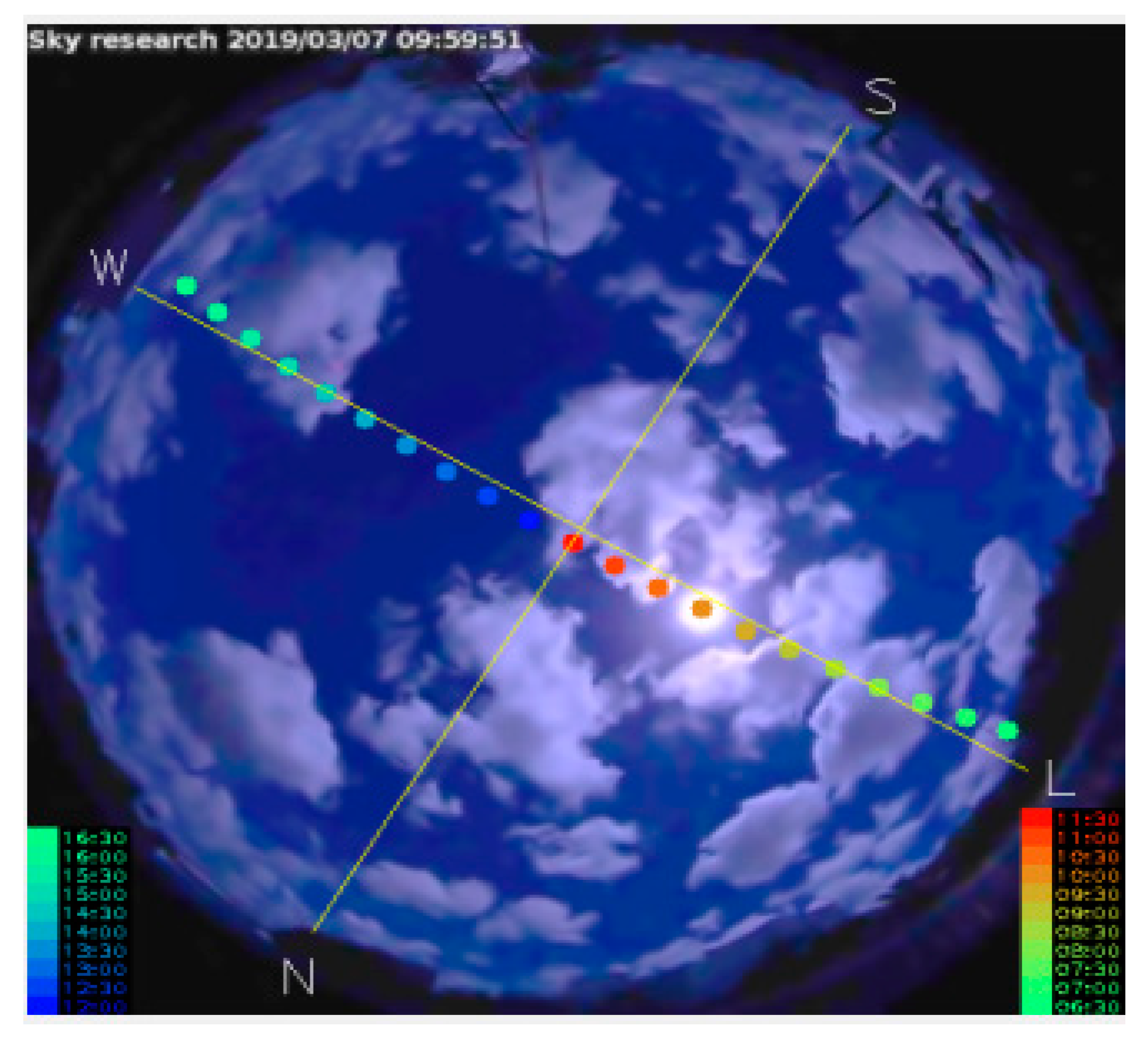
After finishing the calibration process, given that the Sun position angles were determined with help of Reda’s work, a specific algorithm was created to segment the solar disk in the image, as is shown in Figure 6, where several positions throughout the day can be seen.

3.4. GHI Modeling

A problem in estimating GHI was turned into a regression model, where GHI was the output variable and sky image attributes were the input variables. There were, initially, 18 attributes selected as input variables for the models as follows:

• Initially, as the luminance and brightness of the sky have been reported as a function of the zenith angle [35,36], two attributes were included: the sine and cosine of that angle, which is the angle formed between the local vertical and the pixel where the center of solar disk is located. Both attributes were the first ones included in the input vector to the regression model. In addition, the cloud coverage value in percentage was included in the vector, too.
• The next three attributes were obtained as follows: the average gray levels were calculated on three areas which are the solar disk, the cloud segmented region and the sky.
• Once the metrics $f_4$ and $f_6$ in the segmentation stage revealed good correlation between the cloud/sky areas, they were applied to calculate their averages values on the same three previous areas, which returned six more attributes.
• The last six attributes in the input vector came from the Otsu algorithm [37] used to perform segmentation in gray level images, as illustrated in Figure 7. It returns a threshold value that separates pixels into two classes. This threshold is determined by minimizing intra-class intensity variance, or equivalently, by maximizing inter-class variance. Since the coverage of the solar disk (by clouds) has strong influence on the GHI parameters, measures to depict the Sun coverage condition were placed in the input vector. This way, the Otsu method applied on the solar disk (with an aperture of 5.5°) returned the threshold (t) that creates two classes of pixels. The first attribute generated as a result of that algorithm, a/(a + b), measures the relative extent of a class with respect to the total extent of the gray level intensity of the histogram. In addition, each average of gray level in classes 1 and 2, ${\mathsf{\mu }}_1$ and ${\mathsf{\mu }}_2$, also formed part of the input vector. Finally, each one of the following expressions was added: ${\mathsf{\mu }}_1(a/\left(a+b\right)$), ${\mathsf{\mu }}_2(b/\left(a+b\right)$), and ${\mathsf{\mu }}_1\left(a/\left(a+b\right)\right)+{\mathsf{\mu }}_2(b/\left(a+b\right)$).

In order to reduce the dimensionality, the principal component analysis (PCA) method was performed and associated to a technique for automatic choice of dimensionality [38], which returned 17 features as the inputs of the GHI model.

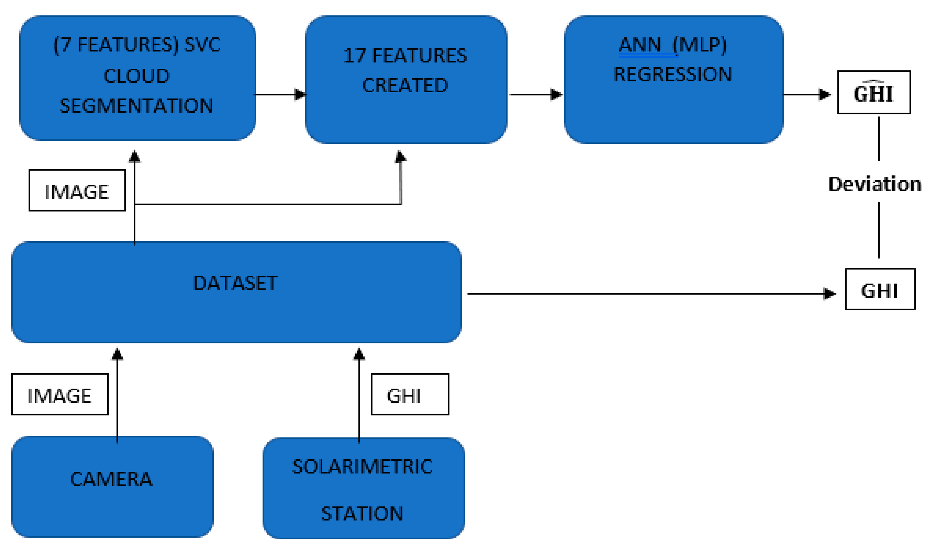
Finally, a model was built based on an artificial neural network (ANN), multilayer perceptron (MLP) type, with 17 inputs (for each feature), hidden layers, and 1 output that represents the GHI to be estimated. In time, it must be observed that the ANN MLP was trained/validated having the GHI signal measured as the target function for each input vector with 17 features. Inside the MLP, the weights were adjusted in the training/validating stages along the neurons in layers to reduce the deviation in the GHI translated into the loss function. Figure 8 is a summary of the path that each sample travels, i.e., image and its respective GHI, both acquired and previously stored in the dataset. The information of the sample continues until it reaches the last point where an estimate, $\widehat{GHI}$, can be compared with the measured GHI. Finally, the deviation is calculated from the GHI truth stored and the $\widehat{GHI}$ inferred by the scheme segmentation -> regression depicted in Figure 8.

4. Results

Most of the period in which the images were collected was under partially cloudy conditions, as shown by the graphic in Figure 9. In the dataset, by consequence, images were recorded with great variability of luminance and contrast among the scenes, which meant a challenge for the regression models. Once the images were taken at several different hours throughout the day, the variability was captured in a high time resolution of 5 s between the images (and their respective irradiances), regarding such sky situations.

The whole set of images had 111,573 samples, while the training/validation set had 89,964 samples as part of the biggest set. An artificial neural network MLP type requires a training set, a validating set, and at least one test set. The training set was formed with data among the 89,964 samples in a total of 80,970 randomly selected. With respect to the validation set, in a similar way it was formed with 8994 samples selected at random, with approximately 10% of the samples reserved for training and validating. Some parameters like root mean square error (RMSE), normalized root mean square error (nRMSE), mean absolute error (MAE), mean bias error (MBE), and normalized mean bias error (nMBE), Equation (13) to Equation (17), as well as the Pearson correlation coefficient, measured the performance of the GHI model during the test stage, immediately after training/validation, for three different test sets. In

Table 3. Results of the metrics applied on the features.

GHI Model	Pearson (%)	RMSE (W/m2)	nRMSE (%)	MAE (W/m2)	MBE (W/m2)	nMBE (%)
Test set	97.4	72.3	12.9	37.9	5.8	1.0
Cloudy day	92.3	50.7	18.7	38.0	0.2	0.08
Partially cloudy day	94.3	99.7	15.5	56.6	−25.6	−3.9

, in the first line there are the results of such metrics over the first test set, built with 9996 samples selected at random regarding several different days and under all sky conditions.

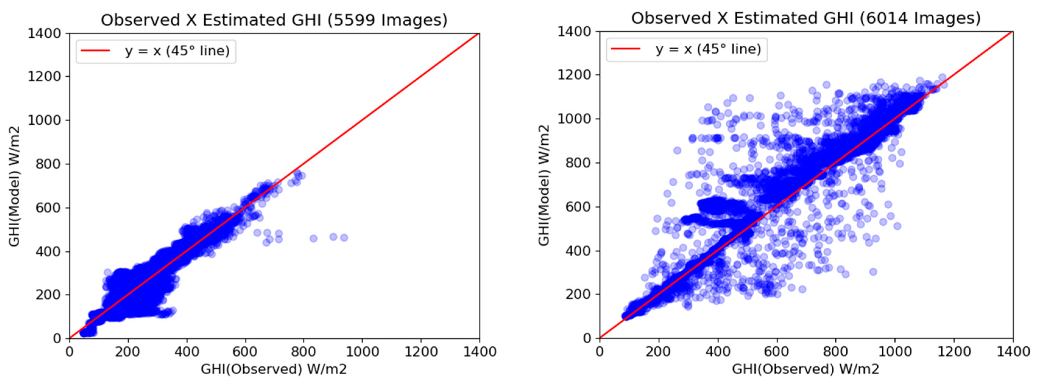
The daily transmittance coefficient Kt, defined as the ratio of terrestrial and extraterrestrial insolation on a horizontal surface, taking into account the totals throughout the day, brings information about the amount of solar energy that reaches the ground. As a consequence, it is known that a low daily Kt value is directly associated with a cloudy day. As Kt rises, partial cloud coverage can be inferred until it reaches, eventually, a clear sky day. This way, two days were also selected for testing: a cloudy day with 5599 samples (Kt equals to 0.29) and a partially cloudy day with 6014 samples (Kt equals to 0.71). Those sampled days, with different sky characteristics picked by their Kt values, were chosen in order to reveal in which conditions the model had a better performance, which cannot be investigated when the samples are mixed at random, as in the first test case. A single day with clear sky throughout the period was not found due to the climate characteristics of that coastal zone, where there is a predominance of partially cloudy days. All the outputs of the regression model, according to the test sets and the metrics used, can be seen in Table 3.

Figure 10 and Figure 11 show the graphics for each test set submitted to the GHI model. In Figure 11, while observing the scattering of points around the line y = x, where the GHI estimates would be the same as the measured values, it is possible to see the higher dispersion in a partially cloudy day regarded the cloudy day, corroborating what is seen by comparing the values of the RMSE metric.

$$RMSE= \sqrt{\frac{1}{N}{\mathsf{\Sigma }}_{i=1}^N{\left(y_i- {\widehat{y}}_i\right)}^2}$$

(13)

$$nRMSE= \frac{\sqrt{\frac{1}{N}{\mathsf{\Sigma }}_{i=1}^N{\left(y_i- {\widehat{y}}_i\right)}^2}}{\frac{1}{N}{\mathsf{\Sigma }}_{i=1}^N\left({\widehat{y}}_i\right)}$$

(14)

$$MAE = \frac{1}{N}{\mathsf{\Sigma }}_{i=1}^N\left(\left|y_i- {\widehat{y}}_i\right|\right)$$

(15)

$$MBE = \frac{1}{N}{\mathsf{\Sigma }}_{i=1}^N\left(y_i- {\widehat{y}}_i\right)$$

(16)

$$nMBE = \frac{\frac{1}{N}{\mathsf{\Sigma }}_{i=1}^N\left(y_i- {\widehat{y}}_i\right)}{\frac{1}{N}{\mathsf{\Sigma }}_{i=1}^N\left({\widehat{y}}_i\right)}$$

(17)

5. Discussion and Conclusions

In this work, a model for estimating GHI irradiances was developed based on images taken from a fish-eye CCTV camera within a high-resolution time period of 5 s. However, due to the excellence in the technical specifications of the observed GHI measurements obtained by the solarimetric station, there was a realistic expectancy that the same accuracy could not be achieved in GHI estimates by the models created.

By explaining the flowchart of the Figure 8 in an upper-left block under cloud segmentation title, that stage was responsible for creating 5 unique features (in a total of 7) used as inputs to a pixel-based SVC machine learning for a binary classification between sky or cloud pixel. With 813 k feature vectors, the segmentation model reached more than 98% success rate in pixel classification, which is comparable to or above the performance of the articles previously seen. As a consequence of the measurement of the number of pixels from sky and from clouds, a method for estimating the cloud coverage has also been developed.

In order to estimate the GHI irradiance, an ANN MLP type regression model was conceived as the next stage after developing 17 new features associated to the cloud segmentation SVC model, which is a novel approach and has not appeared before in the literature to our knowledge. Some of such 17 features are related to the smear in the CMOS image sensor, a problem already seen in other research and coming from the presence of a very bright light [7]. Here it was solved by using special features created in combination with Otsu’s method, a technique used in object clustering inside images. They were computed over the solar disk, and managed to deliver to the MLP model the numerical inputs needed to include the direct irradiance component into GHI. In other words, they consist of six features created on the Otsu’s method to supply the model with information about the fraction of the Sun that is covered/uncovered (by clouds), as well the average of the intensity of the pixels inside the solar disk by separating them in two regions according to the histogram of their bright in gray levels. Those 6 features were later added to another 12 and submitted to the PCA method, resulting in 17 features used as inputs in the artificial neural network MLP for estimating the GHI.

With regard to the results, seen in Table 3, the first test set with 9996 images presented a Pearson’s correlation coefficient of, approximately, 97%, which suggests a high correlation between the estimated and observed GHI data. However, that test set was formed with images selected at random from cloudy and partially cloudy days, given that there were no clear sky days due to the climate of the coastal zone. Then, through that test set, the performance of the model could be evaluated in two different circumstances: a cloudy day and a partially cloudy day. Given that the daily transmittance coefficient, Kt, is an index associated to a cloud coverage along the day, it is accepted in solar research that a Kt < 0.3 means a cloudy day, while a Kt ~ 0.7 means a partially cloudy day. This way, two days, for Kt equals to 0.29 and 0.71, were evaluated. The cloudy day yielded a RMSE for GHI of 50.7 W/m² and nRMSE of 18.7%, while the partially cloudy day yielded a RMSE for GHI of 99.7 W/m² and nRMSE of 15.5%. That indicated a better RMSE performance in a cloudy day (as could be in a clear sky day) just when, by supposition, the GHI signal has less variability. Moreover, in that cloudy day, the average GHI was 271.1 W/m², smaller than 643.2 W/m² of the partially cloudy day. Conversely, the nRMSE was better in a partially cloudy day due to the average GHI, too much higher in that case. The first test set with random samples of several days, despite yielding 12.9% for nRSME and an intermediate value for RMSE of 72.3 W/m², between 50.7 and 99.7W/m², respectively, that cloudy and partially cloudy days, brought no clues about the performance of the model as the day became more or less cloudy.

By comparing to results found in some papers, the nRMSE metric achieved by Kurtz for GHI was 9 to 11% [7], closed to what has been achieved here for (12.9%). The work of Schmidt [13], based on KNN machine learning, had Pearson’s correlation of about 94.1% and higher nRMSE (26.6%) for GHI. By using cloud and Sun segmentation as well as radiation transfer functions, Gauchet reached 17% for nRMSE (with Pearson coefficient of 95.9%) for GHI [12]. However, instead of instantaneous values of irradiances, that work used a 5 min interval of integration. None of the three previous papers cited compared the performance of their models using a partially cloudy day.

It is prudent to note that comparisons between models created under different sky conditions and/or different ways to measure observational data can induce to errors in conclusions. Furthermore, as errors are generally lower under clear or overcast sky condition measurements, the comparison of data from different sites does not constitute conclusive evidence as to which method is superior. Different spectral sensitivity of the reference instrumentation can, as well, complicate comparisons.

Finally, improvements are intended to be done in some stages of this work with the aim to get better performances. Rudy [39], for instance, showed that an approach based on a multifractal analysis can be helpful to study the intermittency of high frequency global solar radiation sequences under a tropical climate, which can lead to an extra characterization of parameters/features in addition to the features already used. Three parameters studied inside that paper have a huge potential to be explored here as inputs into the artificial neural network regression stage.

Eventually, other clustering algorithms for extracting features of Sun coverage can make better contributions than the Otsu method. Other regression algorithms are also intended to be tested to compare their results.