Article

Numerical Study on Anisotropic Influence of Joint Spacing on Mechanical Behavior of Rock Mass Models under Uniaxial Compression

1
State Key Laboratory for Geomechanics & Deep Underground Engineering, China University of Mining and Technology (Beijing), Beijing 100083, China
2
School of Engineering and Technology, China University of Geosciences (Beijing), Beijing 100083, China
*
Author to whom correspondence should be addressed.
Energies 2020, 13(24), 6698; https://doi.org/10.3390/en13246698
Submission received: 22 November 2020 / Revised: 14 December 2020 / Accepted: 15 December 2020 / Published: 18 December 2020
(This article belongs to the Special Issue Sustainable Geotechnical Engineering and Its Applications)

Abstract

:
Mechanical properties of rock masses are dominated by the nonlinear response of joints and their arrangement. In this paper, combined influences of joint spacing (s) and joint inclination angle (β) on mechanical behavior of rock mass models with large open joints under uniaxial compression were investigated by PFC modeling. With a large amount of local measurement circles placed along the pre-defined measurement lines (ML), stresses and joint response parameters at different scales (the measurement circles, the MLs and the whole specimen) were defined and calculated. It was found that macroscopic behaviors of the jointed specimens, such as four types of deformation behaviors, four failure modes, strength, deformability modulus and ductility index, are dominated by nonlinear response of the joint system, especially the interaction between the joints and rock bridges. The joints may experience three stages, i.e., starting to close, closed and opening again. On the joint plane, the peak stresses of the rock bridges and those of the joints may not be reached at the same time; i.e., joint strength mobilization happens with the loss of the rock bridges’ resistance. The influence of s on specimen behavior is little for β = 90°, obvious for β = 0° or 30° and significant for β = 45° or 60°, and this can be related to their different microscopic damage mechanisms.

1. Introduction

Evaluation of mechanical properties of rock masses is of great importance for safe, efficient and sustainable exploitation of underground energy resources (coal, oil and gas, geothermal etc.). In general, the rock mass is weaker, more deformable and permeable, and highly anisotropic than the intact rock due to the presence of joints. The complex nonlinear response of rock joints and diversity of joint arrangement patterns make the prediction of the mechanical behavior of a rock mass be a very challenging and difficult task.
In practical engineering design, a number of rock mass classification schemes have been developed to quantitatively estimate the properties of the in situ rock mass, e.g., RQD (Rock mass Quality Designation) [1], RMR (Rock Mass Rating) [2], Q [3] and GSI (Geological Strength Index) [4,5]. In these rock mass classification systems, a few of the key geometrical parameters of joint network are taken into account individually, such as the number of joint sets, the joint spacing and orientation of joints relative to the structure.
Based on the above-mentioned rock mass classification systems, some empirical relations have been proposed to estimate strength and deformability of jointed rock masses. For example, Hoek and Brown [6,7] developed a well-known strength criterion with two parameters m and s which can be related to the RMR value; Cai et al. [5,8] expressed the peak and residual Hoek–Brown strength parameters as functions of the two GSI values, i.e., joint condition factor Jc and block volume Vb; Bieniawski [9] and Barton et al. [10] suggested a relation between deformation modulus and the RMR and Q value, respectively. In these rock mass classification systems and empirical relations, the influence of joint spacing on properties of rock masses is considered isotropically.
To further understand the dependence of anisotropic mechanical behavior of jointed rock masses on joint configuration, lots of physical model tests have been done under different loading conditions. The samples can be classified into two groups: (1) samples made by assemblages of blocks, to simulate entirely fractured rock masses, and (2) samples made by a single block containing non-persistent fractures, to model rock masses with discontinuous joints.
With assemblages of blocks, Brown and Trollope [11], Einstein and Hirschfeld [12], and Tiwari and Rao [13] have carried out triaxial compression tests to investigate the influence of confining stress, number of joint sets, joint orientation and joint spacing on strength, deformation and failure modes of the jointed specimens; Hayashi [14] has done direct shear tests to study shear strength reduction depending on number of transversal continuous parallel joints; Yang et al. [15] carried out uniaxial compression test to investigate the influence of joint orientation for three sets of joints. It was found that: (1) the strength of the jointed specimen has the upper and lower limits, which is the strength of the intact material and the strength of the crushed material, respectively; (2) the strength decreases while the deformability increases as the joint spacing decreases, which depend on the orientation of the joint plane significantly at low confining pressure; (3) joints will have little influence on the behavior of the jointed specimen at high confining pressure.
Direct shear [16,17], uniaxial compression [18,19,20,21] and biaxial compression [22,23] tests have been done for samples with non-persistent joints. The focus was put on the influence of geometrical parameters of a single joint set, including the joint orientation, spacing, persistence and arrangement pattern. Comparing with assemblages of blocks, the mechanical responses of samples with discontinuous joints are more complex and the anisotropic behaviors are governed by cracking process occurring in the rock matrix, opening/closing or sliding of the pre-existing joints and the interaction between the rock bridges and the joints.
In order to understand the underlying damage mechanism of mechanical behavior of the jointed specimens observed in the physical model tests, numerical studies have been applied in many researches, such as FEM [24], BEM [17], DEM [25], and hybrid FEM/DEM approaches [26].
In the recent decades, Particle Flow Code (PFC), which is a DEM method with assemblies of rigid particles, has been widely used to investigate the damage mechanism of jointed rock masses [27,28,29]. In a particle flow model, the intact material is represented by a group of particles that bonded together. Each bond may break up independently when it’s normal or shear bonding strength is reached, which can directly simulate the two different cracking mechanisms occurring in the matrix, i.e., tensile and shear cracking. Furthermore, with the development of the smooth joint (SJ) contact model, the nonlinear behavior of rock joints can be simulated more accurately [30]. For example, Bahaaddini et al. [31,32] carried out PFC3D modeling for the experiment of Prudencio and Jan [23]. They investigated the dependence of the UCS and deformation modulus on each joint geometrical parameter individually, including the joint dip angle, joint overlap angle, joint orientation and joint spacing. Chiu et al. [33] simulated the test of Yang et al. [15] with PFC3D and achieved improvement in simulating the mixed and sliding failure modes, by developing a modified SJ model with the nonlinear shear strength criterion proposed by Barton and Choubey [34]. Cheng et al. [35] and Chen et al. [36] have done 2D PFC modeling for uniaxial compression tests of the specimens containing non-persistent open joints by Chen et al. [20] and Zhang [21], respectively. In these two studies, the combined variations of joint orientation with joint persistence for small joints or with joint spacing for large joints, were investigated, respectively. They demonstrated that PFC modeling is capable of reproducing multi-peak deformation behaviors observed in the physical experiments for both joint configurations. By analyzing the aperture and normal/shear contact forces of joint systems, the significant influence of the joint strength mobilization on the strength and deformability of the jointed specimens was revealed.
Though the salient influence of joint spacing on properties of jointed rock masses has long been recognized, its anisotropic effect and underlying damage mechanism has not been fully understood, especially about the interaction between joints and rock bridges. In this paper, to fulfill this purpose, measurement circles were used in 2D PFC modeling for the physical model test conducted by Zhang [21]. With a large number of small measurement circles placing on joint planes, stresses and joint response parameters at different scales were firstly defined and calculated. Then, the response of the joint system and interaction of rock bridges and rock joints were analyzed. Finally, the microscopic damage mechanism for combined influence of joint orientation and joint spacing on the mechanical behavior of rock masses was analyzed.

2. Particle Flow Modeling of the Jointed Specimens

2.1. Setup of the Jointed Specimens

Some different materials like mortar, gypsum, etc. can be used for preparing the physical models (Zanelato et al. [37]). To better understand the anisotropic influence of joint spacing on mechanical behavior of jointed rock masses, Zhang [21] performed physical model tests on rock like material containing large non-persistent open joints. Samples were carefully prepared with a mixture of gypsum, Portland cement and water at a weight ratio of 0.99:0.01:0.6. Joints were made by firstly inserting 0.3 mm-thick greased thin nickel alloy strips through precut slots and then removing them later after the setting of the liquid mixture started. The samples were kept at room temperature for 21 days before the mechanical testing. The apparatus used for uniaxial compression tests is an INSTRON 8506 servo-controlled hydraulic loading system. The displacement rate is fixed at 0.0025 mm/s, which corresponds to a constant strain rate of 1.67 × 10⁻⁵ s−1.
The dimension of the specimens is 150 × 150 × 50 mm (height × width × depth). A single set of parallel joints penetrating through the thickness is regularly arranged (see Figure 1). In this study, both joint center distance c (the distance between the two adjacent joints on a joint plane) and joint continuity factor k (the ratio of the length of a single joint to the joint center distance) are fixed, i.e., c = 150 mm and k = 0.8. Accordingly, the joint length is Lj = kc = 120 mm, except for those intersect with the edge of the specimens. The combined variation of the two geometrical parameters, i.e., joint inclination angle β and joint spacing s (the angle between the joint plane and the loading plane, and the distance between the two adjacent joint planes, respectively), are investigated. For jointed specimens, five values of β and three values of s are considered, namely, β = 0°, 30°, 45°, 60° and 90°, and s = 75, 60 and 30 mm. For the intact specimen, s = 150 mm is assumed. Therefore, in total, sixteen joint configurations are included in the physical experiment and PFC modeling (see Table 1).

2.2. Calibration of Micro-Properties in the Numerical Model

In 2D particle flow modeling, a jointed rock mass is simulated by an assemblage of rigid particles bonded together. Contact models for the rock matrix and the joints used in this study are linear parallel bond model and SJ model, respectively. The mechanical behavior of the numerical model is controlled by micro-properties of particles, parallel bonds and SJ contacts.
In general, these micro-properties can be calibrated through a trial-and-error procedure including the two successive steps as follows: (1) Calibration of the micro-properties of particles and parallel bond contacts for the rock matrix, which can be performed by conducting numerical uniaxial compression test for the intact specimen; (2) Calibration of the micro-properties of SJ contacts for the rock joints, which can be carried out based on a series of numerical uniaxial compression tests for the jointed specimens.
Micro-properties for particles, parallel bond contacts and SJ contacts have been calibrated in our previous paper [36], and are listed in Table 2. The macro-properties of the intact specimen obtained by the numerical tests are compared with those by the laboratory tests (see Table 3).

3. Quantities Defined at Different Scales

In the 2D PFC modeling, to investigate the responses of joints and rock bridges on joint planes and their influences on the behavior of jointed specimens, a large number of local measurement circles were placed along the pre-defined measurement lines (ML). Thereafter, quantities were defined at three different scales, i.e., (1) the local measurement circles; (2) the MLs; (3) the whole specimen.

3.1. Quantities in the Local Measurement Circles

In a PFC2D model, microscopic quantities, such as particle displacements, contact forces of bonds or SJ contacts are computed. Since the model is discrete, continuum quantities such as stresses and strain rate do not exist at each point in a particle assembly. Averaging procedures are necessary for transferring from the micro-scale to a continuum. In PFC2D, continuum quantities are defined with respect to a specified measurement area, referred to as “measurement circle” [38] (see Figure 2). By using measurement circles, continuum quantities can be computed and monitored.
The average stress in a measurement circle, σ ¯ i j ( C ) , is defined as:
σ ¯ i j ( C ) = 1 V ( C ) N p σ ¯ i j ( p ) V ( p ) ,
where, V ( C ) is the volume of the measurement circle; N p the number of particles in the measurement circle; V ( p ) and σ ¯ i j ( p ) the volume and the average stress of a particle, respectively.
By defining the porosity, ϕ, as the ratio of total void volume in the measurement circle, V ( C ) can be related to total particle volumes in the region and given by:
V ( C ) = 1 ( 1 ϕ ) N p V ( p ) ,
By applying the Gauss divergence theorem, the average stress of a particle σ ¯ i j ( p ) can be obtained from the forces acting on its contacts as follows:
σ ¯ i j ( p ) = 1 V ( p ) N c ( p ) ( x i ( c )     x i ( p ) ) F i ( c , p ) ,
where, x i ( c ) is the coordinates of the centroid of the particle; N c ( p ) the number of contacts along the surface of the particle; x i ( p ) the coordinates of a contact of the particle; F j ( c , p ) the force acting on a contact of the particle.
Substituting Equations (2) and (3) into Equation (1), the average stress in the measurement circle can be calculated from contact forces of the particles in the region as follows:
σ ¯ i j ( C ) = ( 1 ϕ ) N p V ( p ) [ N p N c ( p ) ( x i ( c ) x i ( p ) ) F j ( c , p ) ] ,
The detailed formulation for the average stress in a measurement circle can be found in the PFC2D User’s Manual [38].
In PFC modeling, a joint segment is composed of SJ contacts between the particles whose centers lying on the opposite sides of the designated joint plane. The response of a SJ contact can be characterized by its microscopic parameters, such as aperture, ratio of closed number and contact forces, etc.
In this study, to evaluate response of a part of joint segment that intersects the measurement circle, the joint response parameters at the scale of a measurement circle were defined as follows:
Average aperture of SJ contacts in a measurement circle ( a ¯ ( C ) ), is defined as:
a ¯ ( C ) = 1 N ( C ) i = 1 N ( C ) a i ,
where, N ( C ) is the number of SJ contacts in the measurement circle; ai the current value for the aperture of the i-th SJ contact. Here, a i > 0 and a i 0 represents that the SJ contact is open or closed, respectively.
Ratio of closed number of SJ contacts in a measurement circle ( R c j ( C ) ), is defined as:
R c j ( C ) = N c j ( C ) N ( C ) ,
where, N c j ( C ) is the number of closed SJ contacts in the measurement circle.
Average normal and shear forces of SJ contacts in a measurement circle ( F ¯ n j ( C ) and F ¯ s j ( C ) ), can be given by:
F ¯ n j ( C ) = 1 N ( C ) i = 1 N ( C ) F n i ,
F ¯ s j ( C ) = 1 N ( C ) i = 1 N ( C ) F n i
where, F n i and F s i are the normal and shear forces acting on the i-th SJ contact, respectively.

3.2. Quantities along the MLs

For each specimen, three pre-defined MLs were installed, and the distance between each of the two adjacent MLs is fixed at 60 mm. For the intact specimen, all three MLs are placed in the material matrix. For the jointed specimens with joint spacing s = 75 mm, the central ML coincides with the single joint plane, while the other two MLs fall in the material matrix. For the jointed specimens with joint spacing s = 60 mm and 30 mm, all three MLs overlaps the joint planes. Figure 3 shows arrangement of measurement circles along the three MLs in specimen E45-3P (β = 45° and s = 60 mm).
The local measurement circles can be classified into three types: (1) J-type measurement circle, which only covers joint segment; (2) R-type measurement circle, which only covers rock bridge segment (or rock matrix); (3) H-type measurement circle, which covers both the joint and the rock bridge segment.
In this study, the diameter of each of these local measurement circles ( D C ), is fixed at 10 mm. The total number of the local measurement circles along a given ML (n), is the summation of the numbers of three types of local measurement circles, which can be given by:
n = n J + n R + n H ,
where, n J , n R and n H are the number of J-type, R-type and H-type measurement circles along the ML, respectively.
For specimens with discontinuous joints, the joint plane can be considered as a combined mechanical system of the two phases, i.e., the rock bridge phase and the joint phase. The two phases are connected in parallel; i.e., the total force applied on the joint plane is the sum of the forces acting on the two phases.
For simplicity, it is assumed that the center of a H-type measurement circle is located at the end of a joint segment, which means that a half of the H-type measurement circle covers the joint segment while the remaining half covers the rock bridge segment. Then the equivalent number of measurement circles of the rock bridge phase and the joint phase along the ML ( n R and n J ) can be calculated as follows:
n R = n R + n H / 2 ,
n J = n J + n H / 2
The lengths of the rock bridge phase, the joint phase and the joint plane ( L ( R ) , L ( J ) and L ), can be related to n R , n J and n as well as the joint continuity factor k and given by:
L ( R ) = ( 1 k ) L = n R D C ,
L ( J ) = k L = n J D C ,
L = n D C
The average normal or shear stresses on the joint plane ( σ ¯ ( J P ) or τ ¯ ( J P ) ) is the mean value of the corresponding stress component obtained from all the local measurement circles along the ML:
σ ¯ ( J P ) = 1 L i = 1 n ( σ ¯ ( C i ) D C ) = 1 n i = 1 n σ ¯ ( C i ) ,  
τ ¯ ( J P ) = 1 L i = 1 n ( τ ¯ ( C i ) D C ) = 1 n i = 1 n τ ¯ ( C i )
where, σ ¯ ( C i ) and τ ¯ ( C i ) are the average normal and shear stresses of the i-th measurement circle along the ML of the joint plane, respectively, which can be calculated by transformation of the average second-order stress tensor σ ¯ i j ( C i ) to the new coordinate system based on the orientation of the joint plane.
Denote σ ¯ ( R ) or τ ¯ ( R ) and σ ¯ ( J ) or τ ¯ ( J ) as the average normal or shear stresses of the rock bridge phase and the joint phase, respectively. Their values can be given by:
σ ¯ ( R ) = 1 n R ( i = 1 n R σ ¯ ( C i ) + 1 2 i = 1 n H σ ¯ ( C i ) ) ,
τ ¯ ( R ) = 1 n R ( i = 1 n R τ ¯ ( C i ) + 1 2 i = 1 n H τ ¯ ( C i ) )
σ ¯ ( J ) = 1 n J ( i = 1 n J σ ¯ ( C i ) + 1 2 i = 1 n H σ ¯ ( C i ) ) ,
τ ¯ ( J ) = 1 n J ( i = 1 n J τ ¯ ( C i ) + 1 2 i = 1 n H τ ¯ ( C i ) )
By substituting Equations (9), (10)–(13) into Equation (11), stresses on the joint plane ( σ ¯ ( J P ) or τ ¯ ( J P ) ) can be related to the corresponding values of the two phases ( σ ¯ ( R ) or τ ¯ ( R ) and σ ¯ ( J ) or τ ¯ ( J ) ) with the joint continuity factor k:
σ ¯ ( J P ) = k σ ¯ ( J ) + ( 1 k ) σ ¯ ( R ) ,
τ ¯ ( J P ) = k τ ¯ ( J ) + ( 1 k ) τ ¯ ( R )
It should be noted that a J-type measurement circle covers not only a part of joint segment but also the matrix on both sides of it (see Figure 2), therefore the average stress of a J-type measurement circle is related to the load carried by the joint as well as its two sidewalls. Correspondingly, σ ¯ ( J ) or τ ¯ ( J ) reflects the comprehensive load-carrying capacity of the joints and their sidewalls.
To evaluate the response of the joint phase on a joint plane, the joint response parameters, i.e., average aperture of SJ contacts on the joint plane ( a ¯ ( J P ) ), ratio of closed number of SJ contacts on the joint plane ( R c j ( J P ) ), and average normal and shear forces of SJ contacts on the joint plane ( F ¯ n j ( J P ) and F ¯ n j ( J P ) ), are defined as follows:
a ¯ ( J P ) = 1 N ( J P ) i = 1 N ( J P ) a i ,
R c j ( J P ) = N c j ( J P ) N ( J P ) ,
F ¯ n j ( J P ) = 1 N ( J P ) i = 1 N ( J P ) F n i ,
F ¯ s j ( J P ) = 1 N ( J P ) i = 1 N ( J P ) F n i
where, N ( J P ) and N c j ( J P ) are the total number of SJ contacts and the number of closed SJ contacts counted within all the measurement circles along the ML of the joint plane, respectively.

3.3. Quantities of the Whole Specimen

In a PFC model, average stress of the whole specimen, σ ¯ i j , can be obtained through the largest measurement circle (the incircle of the square specimen), in which the most area of the specimen is covered (see Figure 3). In addition, axial stress and axial strain of the specimen, σ 1 and ε 1 , can be obtained by monitoring the force and displacement of the top loading platen (the bottom of the specimen is fixed), respectively, to compare with the corresponding quantities measured in the physical model test.
Accordingly, the comprehensive response of joint system can be measured by the joint response parameters, i.e., average aperture, ratio of closed number and average normal or shear forces of SJ contacts in the whole specimen ( a ¯ , R c j , F ¯ n j and F ¯ s j ), which are defined as follows:
a ¯ = 1 N i = 1 N a i ,
R c j = N c j N ,
F ¯ n j = 1 N i = 1 N F n i ,
F ¯ s j = 1 N i = 1 N F n i
where, N and N c j are the total number of SJ contacts and number of closed SJ contacts in the whole specimen, respectively.
To compare the extent of joint strength mobilization in all jointed specimens, average normal and shear forces of SJ contacts in the whole specimen can be normalized and given by:
F ¯ n j N = F ¯ n j / ( F ¯ n j ) max ,
F ¯ s j N = F ¯ s j / ( F ¯ n j ) max
where, ( F ¯ n j ) max is the maximum value of F ¯ n j in all jointed specimens, which occurs in specimen E0-1P (β = 0° and s = 75 mm) for this study; F ¯ n j N and F ¯ s j N normalized average normal and shear forces of SJ contacts in the whole specimen, respectively.

4. Results and Discussion

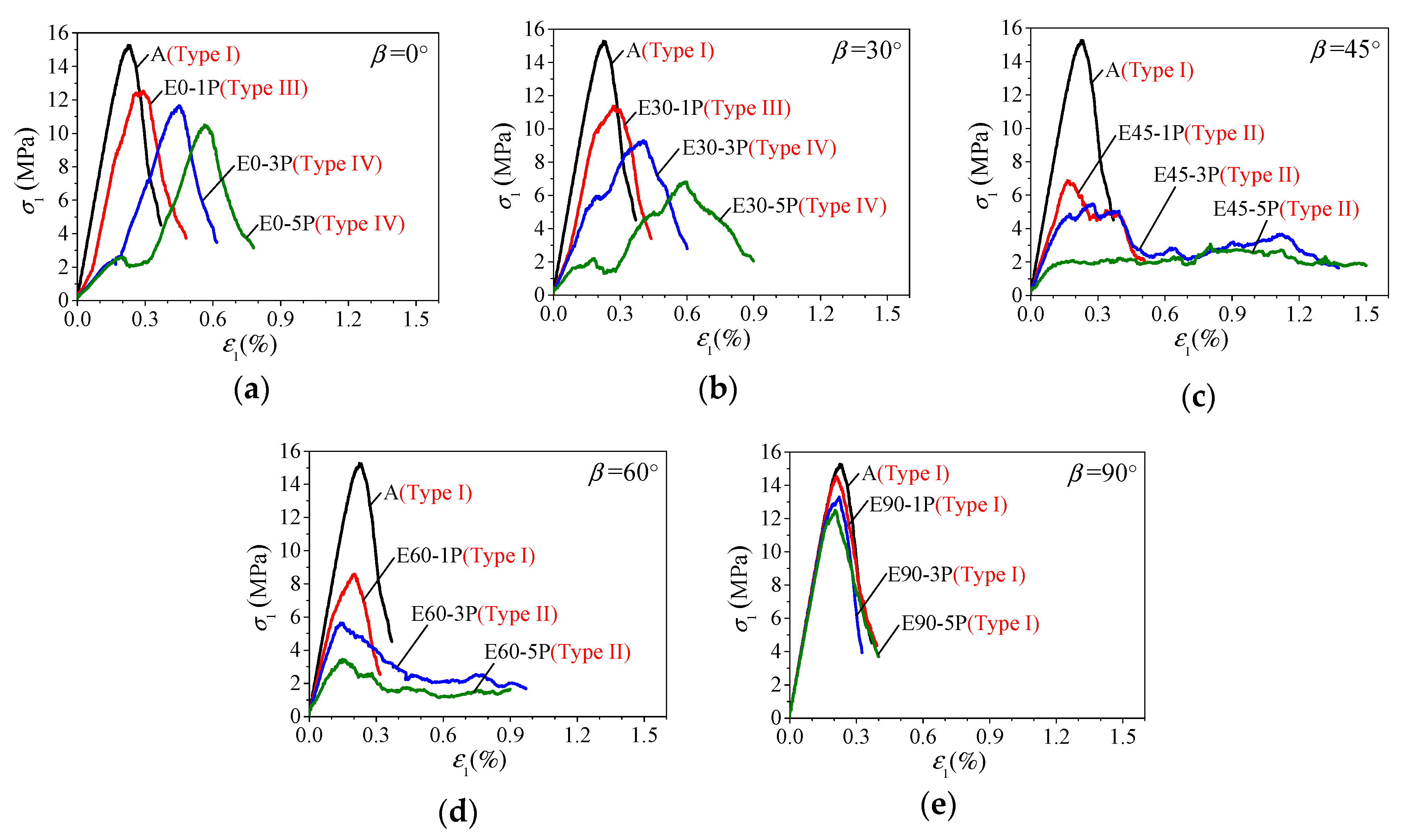
4.1. Macroscopic Mechanical Response of Jointed Specimens

The complete axial stress–strain curves ( σ 1 vs. ε 1 ) of all specimens obtained from PFC modeling are presented in Figure 4. Four types of deformation behaviors, namely, Type I-strain softening after the single peak, Type II-general strain softening with oscillations, Type III-yield platform-strain softening and Type IV-yield platform-strain hardening-strain softening, were observed. They are classified according to different stages occurred after the first peak [20]. The delaying or elongation of strain softening stage in these multi-peak curves (Types II–IV) increases the ductility of the jointed specimen.
Type I deformation behavior, i.e., the single peak curve, was observed in the intact specimen (A), specimens with vertical joints (E90-1P, E90-3P and E90-5P) and specimen E60-1P. Type II deformation behavior occurred in specimens with β = 45° and specimens with β = 60° at medium or small joint spacing (s = 60 and 30 mm), i.e., E45-1P, E45-3P, E45-5P, E60-3P and E60-5P. Type III deformation behavior was observed in specimens with β = 0° and 30° at large joint spacing (s = 75 mm), i.e., E0-1P and E30-1P, while Type IV deformation behavior in those at medium or small joint spacing (s = 60 or 30 mm), i.e., E0-3P, E0-5P, E30-3P and E30-5P.
Figure 5 shows the failure phenomena at the end of the physical tests for all jointed specimens. In total, four failure modes were identified, i.e., Mode A: axial cleavage, Mode B: crushing, Mode C: stepped failure and Mode D: shear failure.
Failure Mode A can always be observed in the intact specimen (A) and specimens with vertical joints (E90-1P, E90-3P and E90-5P). For this failure mode, tensile cracks initiated from joint tips or matrix propagate vertically and finally split specimens into several strips. Most of the joints keep opening while some of them close partially due to Poisson’s effect.
Failure Mode B occurs in the specimens with horizontal joints (E0-1P, E0-3P and E0-5P) or specimens with β = 30° at s = 75 mm and 60 mm (E30-1P and E30-3P), where tensile cracks propagated along loading direction and the entire closure of all joints leads to crushing of the matrix around joints.
Failure mode C occurs in specimen E30-5P, E45-3P, E45-5P, E60-3P and E60-5P. For that mode, stepped failure planes are formed by connection of adjacent wing cracks and the pre-existing joints. Some joints close partially, while others open significantly due to sliding of these stepped planes (secondary shear cracks developed in rock bridges simultaneously).
Failure mode D occurs in specimen E45-1P and E60-1P, where quasi-coplanar shear cracks link with joints and form a single failure plane, and the failure of the specimen is caused by sliding along that plane. Joints close partially in specimen E45-1P while keep opening in specimen E60-1P.
Figure 6, Figure 7 and Figure 8 plot the normalized peak strength (σJR/σR), the normalized deformability modulus (EJR/ER) and the last peak strain (εf2) vs. the two joint geometrical parameters (β and s). Here, σJR and σR are the peak strength of the jointed specimens and that of the intact specimen, respectively; EJR and ER the deformability modulus of the jointed specimens and that of the intact specimen, respectively. In PFC modeling, deformability modulus is taken as the tangent modulus at 50% of peak strength in the stress–strain curve, can be used to characterize deformability at elastic stage in the most cases. The last peak strain εf2 is the strain at the last peak stress, which is served as a ductility index to characterize inelastic deformability of multi-peak curves [20].
It can be seen that: (1) at each joint spacing s, σJR/σR vs. β are V-shaped or U-shaped curves with the minima at β = 45° or 60°, EJR/ER increases with β and εf2 vs. β are inverted V-shaped curves with the maxima at β = 45°; (2) for a given joint inclination angle β, σJR/σR and EJR/ER increase with s while εf2 decrease with s.

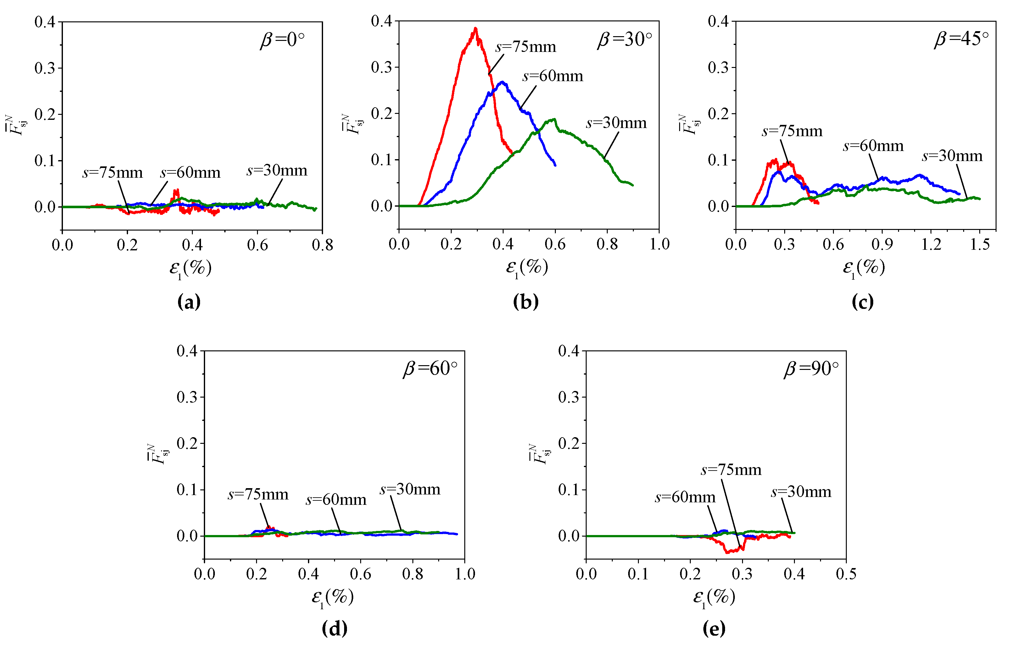
4.2. Overall Response of the Joint System

Figure 9, Figure 10, Figure 11 and Figure 12 show evolution of the joint response parameters of the whole specimen for all jointed specimens, i.e., average aperture, ratio of closed number, and normalized average normal and shear forces of SJ contacts in the whole specimen ( a ¯ , R c j , F ¯ n j N and F ¯ s j N ). It should be noted that the initial value of a ¯ (a0), equals to 0.1 mm.
In general, originally opened SJ contacts may experience three stages sequentially: (1) some of SJ contacts may start to close but none of them closed completely and they cannot transfer any normal or shear forces, lead to decrease in a ¯ and remaining zero values of R c j , F ¯ n j N and F ¯ s j N ; (2) these SJ contacts closed completely and can transfer normal or shear forces, lead to reaching of the minimum for a ¯ and the maximum for R c j , F ¯ n j N and F ¯ s j N ; (3) some of the previously closed SJ contacts may open again or those kept opening opened wider, lead to increase in a ¯ and decrease in R c j , F ¯ n j N and F ¯ s j N .
Figure 13 plots the variation of these joint response parameters at Point F vs. β. At peak strength, it can be seen that: (1) at each joint spacing s, a ¯ increase with β in general while R c j and F ¯ n j N decrease with β, and the curves of F ¯ s j N vs. β are inverted V-shaped with the maxima at β = 30°; (2) for a given joint inclination angle β, a ¯ decrease with s while R c j , F ¯ n j N and F ¯ s j N increase with s; (3) joint strength immobilized for β = 90° or 60°, while slightly, moderately and significantly mobilized for β = 45°, β = 30° and β = 0°, respectively. For example, the values of F ¯ n j N are less than 0.008 and equal to zero for β = 90° and 60°, respectively; they varied from 0.06 to 0.10, 0.36 to 0.67, and 0.83 to 1.0 for β = 45°, β = 30° and β = 0°, respectively.
Figure 14 plots the evolution of F ¯ n j N , F ¯ s j N and σ 1 in the four jointed specimens with different types of deformation behaviors, i.e., specimens E90-5P (Type I), E45-3P (Type II), E0-1P (Type III) and E0-5P (Type IV). Here, characteristic points in σ 1 ε 1 curves can be denoted as: Point O, the beginning of the test; A and B, the start and the end of the linear elastic stage, respectively; F1 and F2, the first and the last peak in multi-peak curves, respectively; F, the peak strength; S, the end of the test. It can be found that the nonlinear and inelastic response of jointed specimens is closely related to that of joint system, where the peaks of F ¯ n j N or F ¯ s j N coincide with the peaks of σ 1 after Point F1. For specimen E90-5P with Type I deformation behavior, normal strength of joint system is mobilized very little right after peak strength (Point F). For specimen E45-3P with Type II deformation behaviors, normal as well as shear strength of joint system are mobilized right after the first peak (Point F1). For the two specimens with horizontal joints at different joint spacing, mobilization of joint normal strength starts very early right after Point A (the start of elastic stage) or very late after Point F1, leads to Type III deformation behavior in specimen E0-1P (s = 75mm) or Type IV deformation behavior in specimen E0-5P (s = 30 mm), respectively.

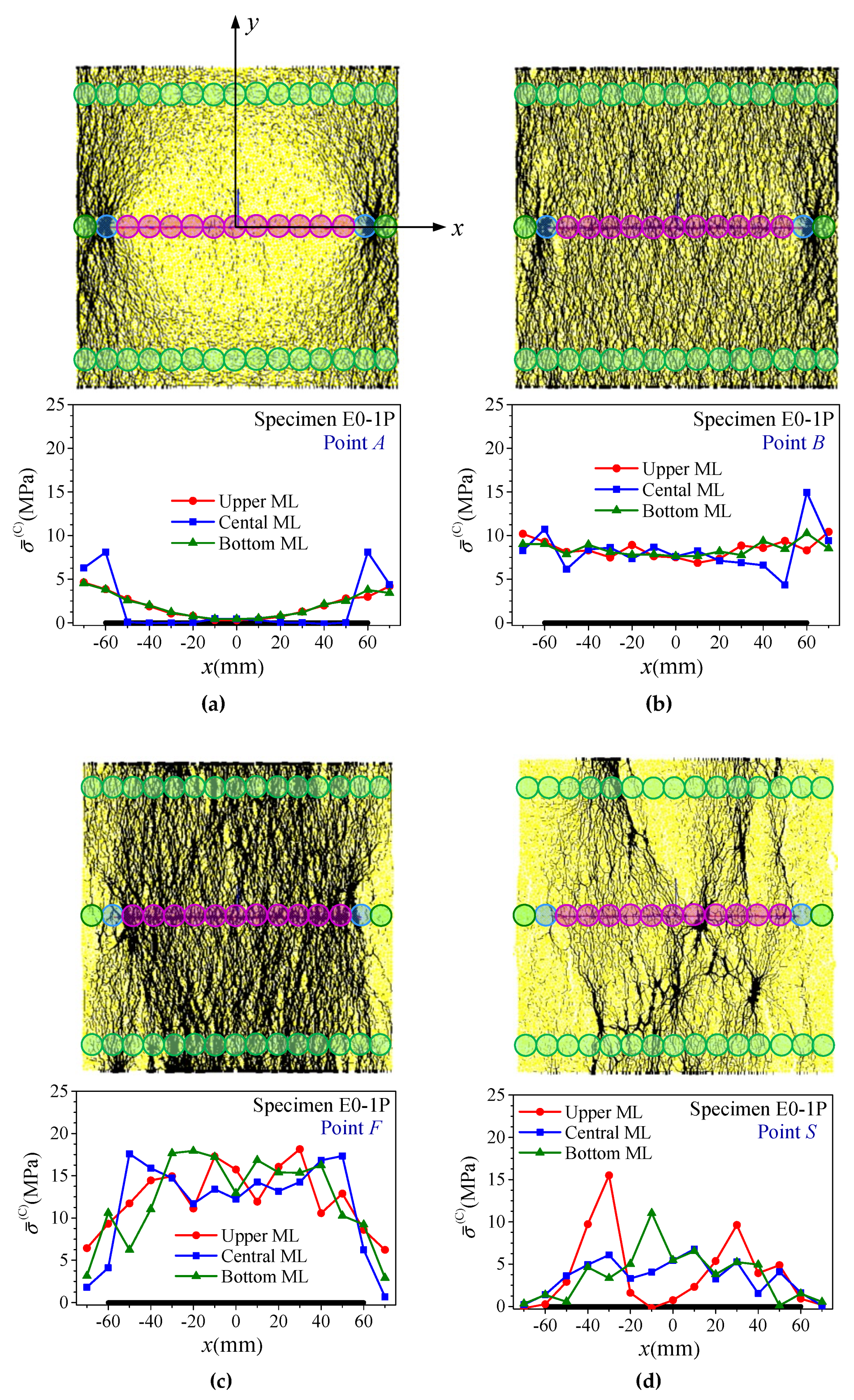
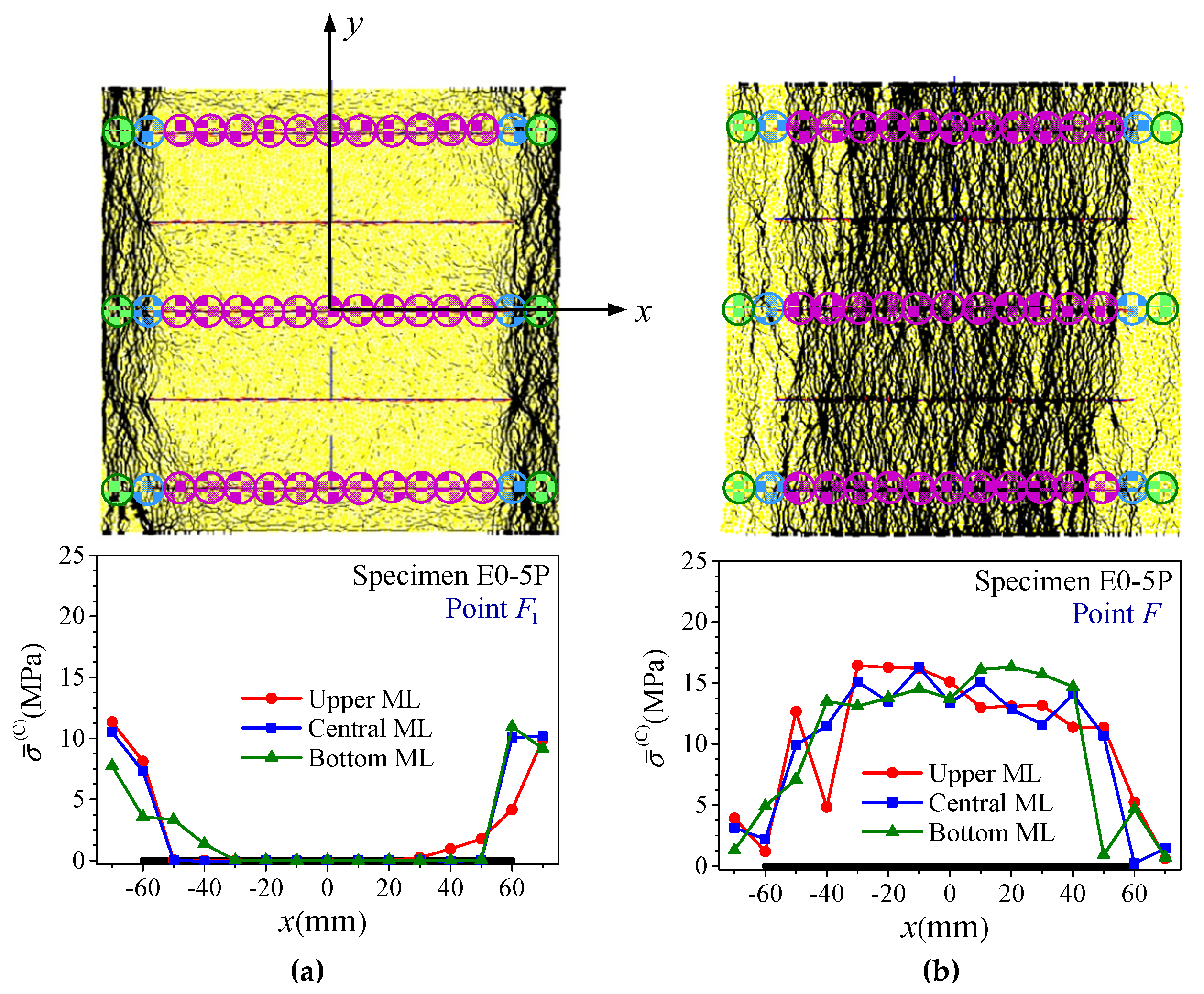
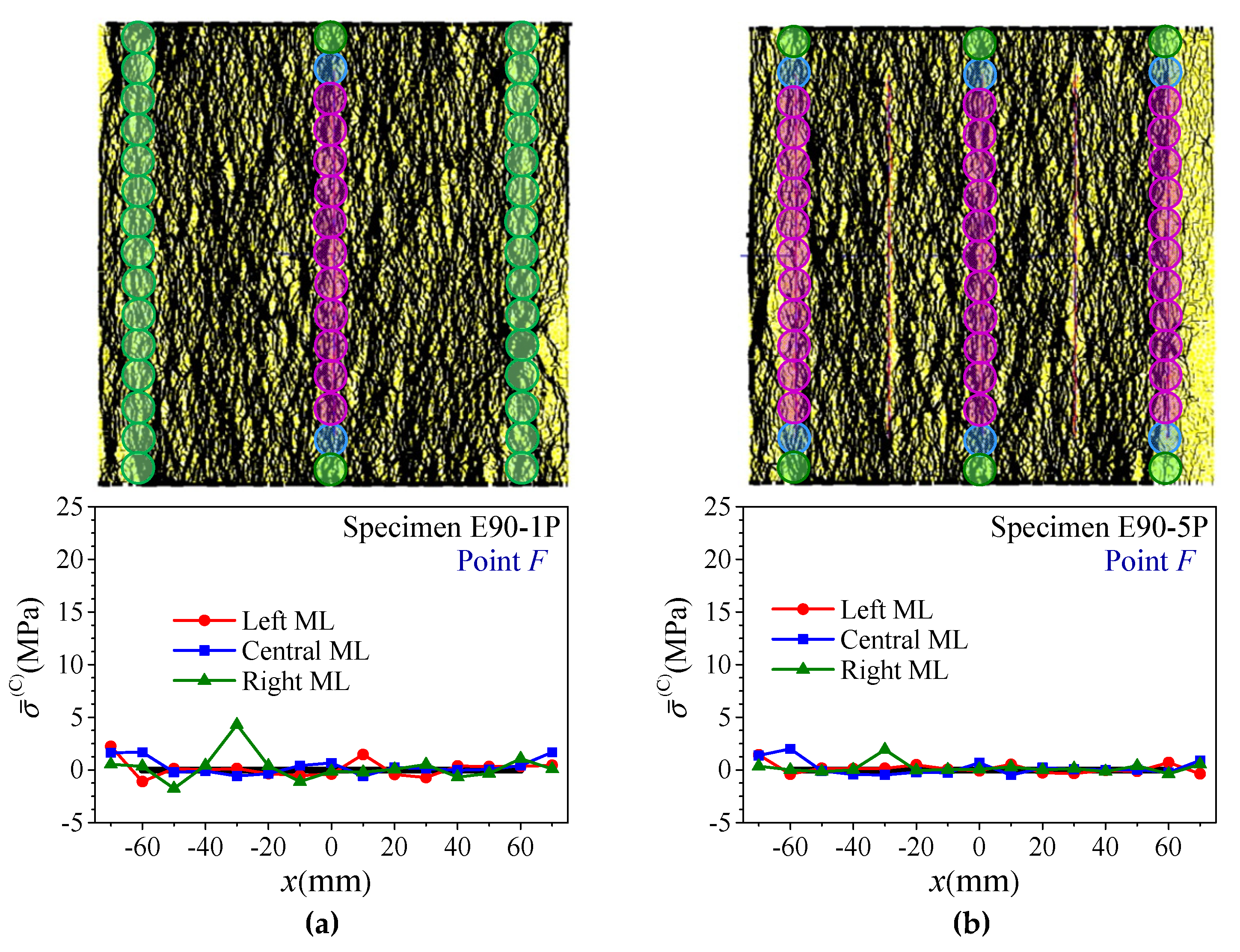
4.3. Response of Rock Bridges and Joints on the Joint Planes

For the intact specimen (A) at Point F and S, Figure 15 shows distributions of contact force chain and the average normal stresses in the local measurement circles ( σ ¯ ( C ) ) along the three MLs. Here, x is the distance from the center of the measurement circle to the center of the ML. In a picture of contact force chain, the resultant forces acting on contacts are indicated by the black bars whose thickness is proportional to the force magnitude. It can be seen that the contact forces almost evenly distributed in the specimen at peak strength (Point F), while it concentrated in the middle region at the end of the test (Point S) due to severe damage of the matrix. Distribution of σ ¯ ( C ) along the upper, central and bottom MLs matches with the picture of contact force chain, namely, larger σ ¯ ( C ) means that the measurement circle locates at a region with concentration of contact force and vice versa.
Figure 16 shows distributions of contact force chain and σ ¯ ( C ) along the three MLs for specimen E0-1P (β = 0° and s = 75 mm) at Point A, B, F and S. At the start of elastic stage (Point A), a load-carrying arch formed around the originally open joint, and the load on the joint plane was only carried by the rock bridges with stress concentration occurring at joint tips. At the end of elastic stage (Point B), the load-carrying arch disappeared and the contact forces almost evenly distributed in the specimen, and the load on the joint plane was carried by the joint and the rock bridges together. At the peak strength (Point F), the rock bridges unloaded entirely while contact forces evenly distributed in the remaining region, and the load on the joint plane was only carried by the joint. At the end of test (Point S), contact forces distributed unevenly due to damage localization of the matrix, and the load on the joint plane was still only carried by the joint.
Figure 17 shows distributions of contact force chain and σ ¯ ( C ) along the three MLs in specimen E0-5P (β = 0° and s = 30 mm) at Point F1 and (b) Point F2 (F). At the first peak (Point F1), load-carrying arches around each joint overlapped and contact forces was mainly distributed in the rock bridges at the left and right edges of the specimen, and the loads on the three joint planes were carried mainly by the rock bridges while only a few of them was transferred by some part of the joints, for example, the right end of the joint on the upper joint plane and the left end of the joint on the bottom joint plane. At the last peak (Point F2, coincide with F), load-carrying arches disappeared and contact forces evenly distributed in the region that directly above and below joints, and loads on the joint planes almost totally carried by the joints while the rock bridges almost unloaded entirely.
Figure 18 shows distributions of contact force chain and σ ¯ ( C ) along the three MLs at Point F for specimens with vertical joints (β = 90°) at s = 75 and 30 mm, i.e., E90-1P and E90-5P. At peak strength, the contact forces almost evenly distributed in the two specimens except for the right edge of specimen E90-5P where the matrix unloaded entirely, and there are very small normal stresses on the three MLs of joint planes.
Figure 19 shows distributions of contact force chain and the average normal and shear stresses in the local measurement circles ( σ ¯ ( C ) and τ ¯ ( C ) ) along the three MLs at Point F for specimens with β = 30° at s = 75 and 30 mm, i.e., E30-1P and E30-5P. For specimen E30-1P at peak strength, contact forces almost evenly distributed in the region above and below the joints while unloading occurred on the two rock bridges especially that on the left side. For specimen E30-5P at peak strength, contact forces distributed very unevenly and concentrated in the middle part. On the central MLs of the two specimens, the normal and shear stresses on the left rock bridges are much lower than those on the right rock bridges as well as those on the joints, which may be caused by sliding along joint planes.
Figure 20 shows distributions of contact force chain and σ ¯ ( C ) and τ ¯ ( C ) on the three MLs at Point F for specimens with β = 45° at s = 75 and 30 mm, i.e., E45-1P and E45-5P. For specimen E45-1P at peak strength (coincide with F1), load-carrying arches around the joints have not disappeared completely, normal and shear stresses on the central joint plane were mainly concentrated in the rock bridges while only a small amount of them were carried by the middle part of the joints. For specimen E45-5P at peak strength (between Point F1 and F2), the contact forces distributed unevenly in the specimen, and normal and shear stresses on the central joint plane distributed like a saw-tooth which may cause by sliding along joint planes.
Figure 21 shows distributions of contact force chain and σ ¯ ( C ) and τ ¯ ( C ) along the three MLs at Point F for specimens with β = 60° at s = 75 and 30 mm, i.e., E60-1P and E60-5P. For the two specimens at peak strength (Point F coincide with F1), load-carrying arches around the joints still existed and normal and shear stress on the central joint plane was totally carried by the rock bridges.
Figure 22 depicts distributions of ratio of closed number of SJ contacts in measurement circles ( R cj ( C ) ) along the central ML at Point F for all jointed specimens. At peak strength, it can be seen that: (1) most of the SJ contacts along the ML closed for specimens with β = 0° and 30° (except for those on the joint tips), and majority of the SJ contacts in the middle of the ML closed for specimens with β = 45°, while none of them and a little of them closed for specimens with β = 60° and β = 90°, respectively; (2) for a given joint inclination angle β, R cj ( C ) decrease with joint spacing s in general.
Figure 23 shows the evolution of the average normal stresses of the rock bridge phase, the joint phase and the joint plane ( σ ¯ ( R ) , σ ¯ ( J ) and σ ¯ ( J P ) ) of the central ML and the axial stress of the specimen ( σ 1 ) in the four typical jointed specimens with different types of deformation behaviors.
For each specimen, σ ¯ ( R ) ε 1 curves are single-peak while the types of σ ¯ ( J ) ε 1 and σ ¯ ( J P ) ε 1 curves are the same as that of σ 1 ε 1 curve; the peak of σ ¯ ( R ) always reaches earlier than the peaks of σ ¯ ( J ) ; i.e., strength mobilization of the joint phase happens after sufficiently consumption of resistance of the rock bridge phase; σ ¯ ( J P ) ε 1 curve is between that of rock bridge and joint (the average normal stress of the joint plane is a weighted average of that of the two phases on the joint plane, see Equation (14a)), and is very close or proportional to σ 1 ε 1 curve σ ¯ ( J P ) should equal to the projection of σ 1 on that plane for a homogenous elastic continuum).
The key points in σ ¯ ( R ) ε 1 and σ ¯ ( J ) ε 1 curves match very well with the characteristic points in σ 1 ε 1 curves as well as σ ¯ ( J P ) ε 1 curves. For example: (1) the peak of σ ¯ ( R ) occurred very close to Point F in specimen E90-5P (Type I), F1 in specimens E45-3P (Type II) and E0-5P (Type IV), and B (the end of elastic stage) in specimen E0-1P (Type III), respectively; (2) the first or the last peak of σ ¯ ( J ) happened nearby Point F or F2 of the specimens with multi-peak axial stress-strain curves, i.e., Type II to IV deformation behaviors.
Table 4 summarized the variation trends of σ ¯ ( R ) , σ ¯ ( J ) and σ ¯ ( J P ) of the central ML and σ 1 for the specimens with the four types of deformation behaviors at each deformation stage; namely, elastic deformation stage (OB), strain hardening stage before the first peak or the single peak (BF1 or BF), yield platform stage(F1F2) and strain softening stage (FS or F2S).
The interaction between the two phases on the joint plane can be divided into three stages: (1) elastic deformation dominated stage (OF, OB or OF1), i.e., before the peak of σ ¯ ( R ) , the rock bridge phase carries most of the load while the joint phase carries a little amount of the load or even no load, due to opening of majority of the SJ contacts; (2) inelastic deformation developing stage (BF2 or F1F2), i.e., between the peak of σ ¯ ( R ) and the last peak of σ ¯ ( J ) , the two phases carry load together (load-carrying capacity of rock bridge decreases while that of joint increases, due to gradual damage of rock bridge and closure of joint, respectively); (3) residual deformation stage (F2S), i.e., after the last peak of σ ¯ ( J ) , the joint phase carries most of load while the rock bridge phase almost unload entirely.
Figure 24 plots the average normal and shear stresses of the rock bridge phase, the joint phase and the joint plane of the central ML at Point F vs. β. At peak strength, it was found that: (1) at each joint spacing s, τ ¯ ( R ) vs. β, τ ¯ ( J ) vs. β, τ ¯ ( J P ) vs. β and σ ¯ ( R ) vs. β are inverted V-shaped curves with the maxima at β = 30° or 45°, while σ ¯ ( J ) and σ ¯ ( J P ) decreases with β; (2) for a given joint inclination angle β, all these stresses increase with s.

4.4. Discussion on Anisotropic Damage Mechanisms

Based on the above analyses, anisotropic influence of joint spacing (s) on behavior of the jointed specimens and their different damage mechanism can be explained as follows:
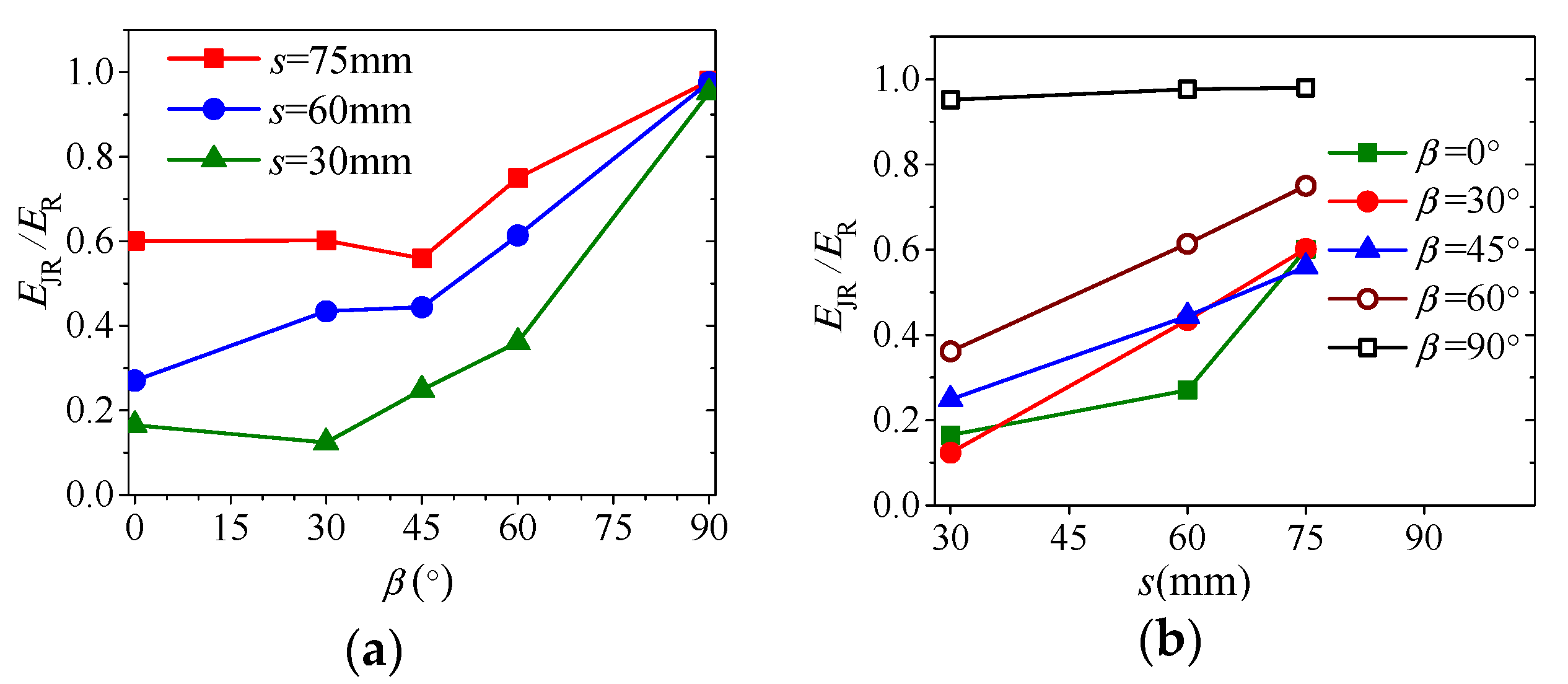
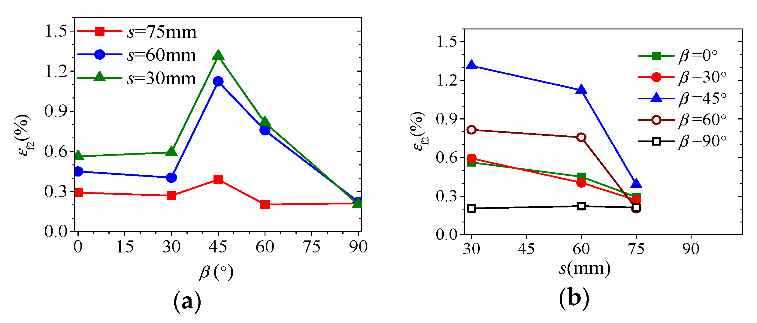
  • For specimens with vertical joints (β = 90°), s has very little influence on their behavior. Since vertical joints are parallel to the loading direction, responses of joints are irrelevant to axial deformation and load transferring, leading to almost no alteration on the normalized Young’s modulus (EJR/ER) and the last peak strain (εf2) and slight increase in the normalized peak strength (σJR/σR) with s. The mechanical behavior of these specimens is the same as those of the intact specimen, i.e., Type I deformation behavior and failure mode A (axial cleavage).
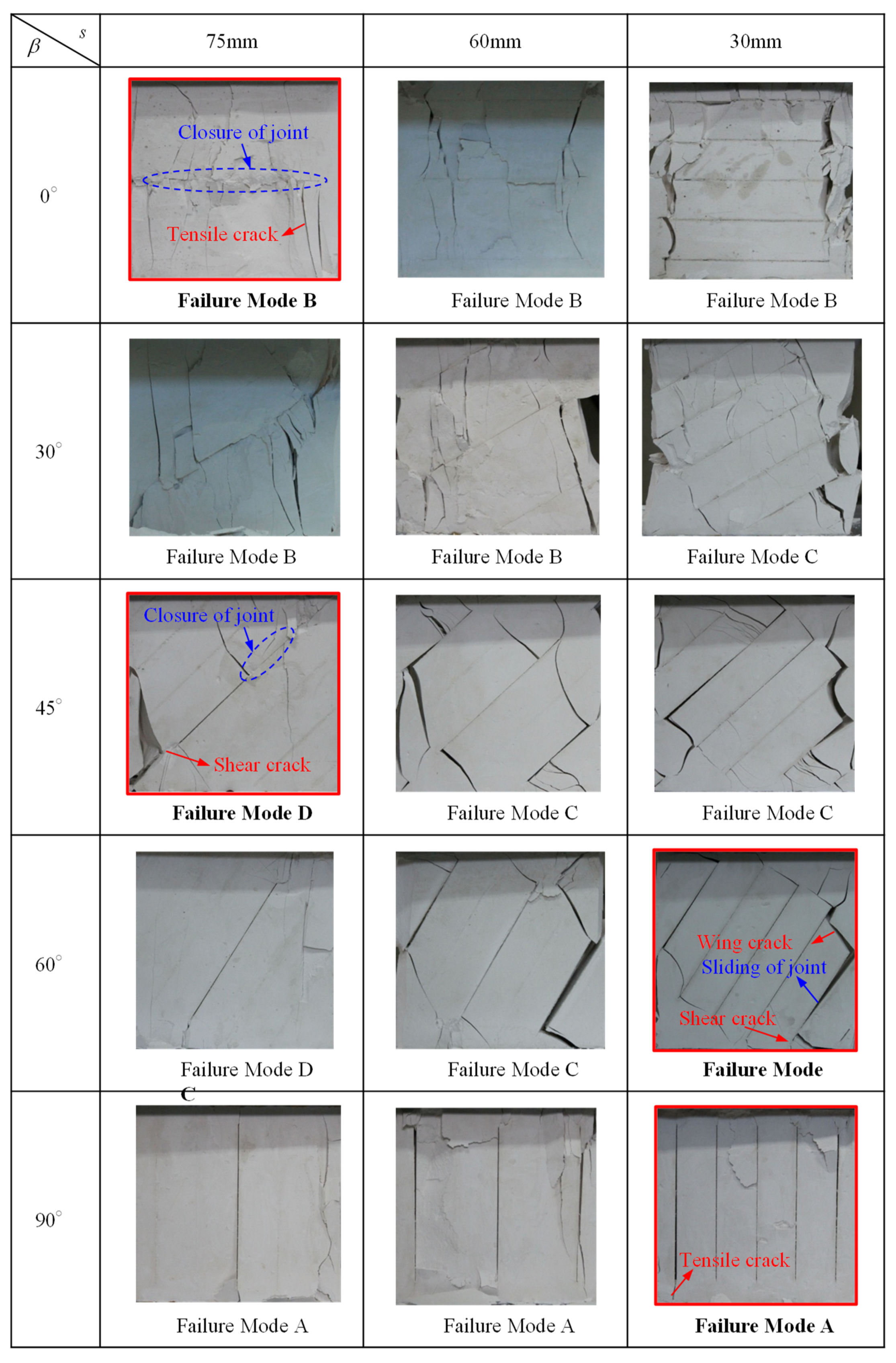
  • For specimens with β = 0° and 30°, s has salient influence on their behavior, especially on the deformability modulus. Before peak strength, gradual closure of most or the majority of originally open joints in these specimens contributes greatly to the increase in deformability, leading to rapid increase in EJR/ER with s. After peak strength, most or the majority of the joints closed entirely and the strengths of the joint system are mobilized fully or saliently, leading to Type III or IV deformation behavior and failure Mode B or C, and moderate increase in σJR/σR and decrease in εf2 with s.
  • For specimens with β = 45° and 60°, s has significant influence on their behavior, especially on the strength and ductility. Before peak strength, gradual closure of minority of the joints or decreasing of joint aperture in these specimens, leads to salient increase in EJR/ER with s. At peak strength, some of the joints closed partially or none of them closed with slight mobilization or immobilization of joint strength, leading to the lowest strength in these specimens and fast increase in σJR/σR with s. After peak strength, shear failure of rock bridges and sliding along joint planes (failure Mode C or D) may lead to Type II deformation behavior and fast decrease in εf2 with s.

5. Conclusions

PFC modeling was used to investigate combined influence of joint spacing (s) and joint inclination angle (β) on mechanical behavior of specimens with large open joints under uniaxial compression. By setting a large amount of local measurement circles on the MLs, stresses and joint response parameters at different scales (the measurement circles, the MLs and the whole specimen) were firstly defined and calculated. Then, the response of the joint system and interaction between rock bridges and joints on the joint planes were analyzed to understand the anisotropic microscopic damage mechanism. The following conclusions can be made:
  • In general, macroscopic behaviors of the jointed specimens, such as four types of deformation behaviors, four failure modes, strength, deformability modulus and ductility index, are dominated by the nonlinear response of joint system, especially the interaction between the joints and rock bridges on the joint planes.
  • The response of joint system can be measured by evolution of the four joint response parameters, i.e., average aperture, ratio of closed number, and normalized average normal and shear forces of SJ contacts in the whole specimen ( a ¯ , R c j , F ¯ n j N and F ¯ s j N ). The joint system may experience three stages, i.e., starting to close, closed and opening again. At peak strength, for each s, a ¯ increases with β while R c j and F ¯ n j N decrease with β, and the curves of F ¯ s j N -β are inverted V-shaped with the maxima at β = 30°; for a given β, a ¯ decreases while R c j , F ¯ n j N and F ¯ s j N increase with s;
  • On the joint plane, the peak stresses of the two phases, i.e., the rock bridge phase and the joint phase, may not be reached at the same time. The interaction between the two phases on the central joint plane can be divided into three stages, i.e., (I) elastic deformation dominated stage (before the peak stress of the rock bridge phase), in which the rock bridge phase carries most of the load, (II) inelastic deformation developing stage (between the peak stress of the rock bridge phase and the last peak stress of the joint phase), in which the two phases carry the load together, and (III) residual deformation stage (after the last peak stress of the joint phase), in which the joint phase carries most of the load.
  • The influence of s on specimen behavior is little for β = 90°, obvious for β = 0° or 30° and significant for β = 45° or 60°, and this can be related to their different damage mechanisms. For β = 90°, load transferring will not be interrupted by vertical joints and, therefore, s has very little influence on specimen behavior; for β = 0° or 30°, entire closure of the majority of pre-existing open joints and significant mobilization of joint strength leads to a fast increase in the normalized deformability modulus (EJR/ER) with s, and moderate increase in the normalized strength (σJR/σR) and decrease in the last peak strain (εf2,) with s; for β = 45° or 60°, strong interruption of load transferring by keeping open the majority, or all, of the joints with slight mobilization or immobilization of joint strength, leading to the lowest strength, salient increase in EJR/ER with s, and fast increase in σJR/σR and decrease in εf2 with s.

Author Contributions

X.C. designed the numerical experiment, proposed the concept, analyzed the data and wrote the manuscript; Z.F. performed the numerical experiments and analyzed the data; C.C. analyzed the data and revised the manuscript. All authors have read and agreed to the published version of the manuscript.

Funding

This research work is financially supported by National Natural Science Foundation of China (No. 11572344 and No. 41941018) and National Key Research and Development Program of China (No. 2016YFC0600901).

Acknowledgments

H. Qian from Institute of Crustal Dynamics, China Earthquake Administration is appreciated here for his support in PFC modeling.

Conflicts of Interest

On behalf of all authors, the corresponding author states that there is no conflict of interest.

References

  1. Deere, D.U.; Hendron, A.J.; Patton, F.D.; Cording, E.J. Design of surface and near surface constructions in rock. In Proceedings of the 8th US Symposium on Rock Mechanics, Minneapolis, MN, USA, 15–17 September 1967; pp. 237–302. [Google Scholar]
  2. Bieniawski, Z.T. Determining rock mass deformability: Experience from case histories. Int. J. Rock Mech. Min. Sci. 1978, 15, 237–247. [Google Scholar] [CrossRef]
  3. Barton, N.; Lien, R.; Lunde, J. Engineering classification of rock masses for the design of tunnel support. Rock Mech. 1974, 6, 189–236. [Google Scholar] [CrossRef]
  4. Hoek, E.; Kaiser, P.K.; Bawden, W.F. Support of Underground Excavations in Hard Rock; Balkema, Ed.; Taylor & Francis: Rotterdam, The Netherlands, 1995. [Google Scholar]
  5. Cai, M.; Kaiser, P.K.; Uno, H.; Tasaka, Y.; Minami, M. Estimation of rock mass deformation modulus and strength of jointed hard rock masses using the GSI system. Int. J. Rock Mech. Min. Sci. 2004, 41, 3–19. [Google Scholar] [CrossRef]
  6. Hoek, E.; Brown, E.T. Empirical strength criterion for rock masses. J. Soil Mech. Found Div. ASCE 1980, 106, 1013–1035. [Google Scholar]
  7. Hoek, E.; Brown, E.T. Practical estimates of rock mass strength. Int. J. Rock Mech. Min. Sci. 1997, 34, 1165–1186. [Google Scholar] [CrossRef]
  8. Cai, M.; Kaiser, P.K.; Tasaka, Y.; Minami, M. Determination of residual strength parameters of jointed rock masses using the GSI system. Int. J. Rock Mech. Min. Sci. 2007, 44, 247–265. [Google Scholar] [CrossRef]
  9. Bieniawski, Z.T. Engineering Rock Mass Classifications; John, W., Ed.; Butterworth-Heinemann: New York, NY, USA, 1989. [Google Scholar]
  10. Barton, N.; Bandis, S.; Bakhtar, K. Strength, deformation and conductivity coupling of rock joints. Int. J. Rock Mech. Min. Sci. Geomech. Abstr. 1985, 22, 121–140. [Google Scholar] [CrossRef]
  11. Brown, E.T.; Trollope, D.H. Strength of a model of jointed rock. J. Soil Mech. Found Div. ASCE 1970, 96, 685–704. [Google Scholar]
  12. Einstein, H.H.; Hirschfeld, R.C. Model studies on mechanics of jointed rock. J. Soil Mech. Found Div. ASCE 1973, 99, 229–248. [Google Scholar]
  13. Tiwari, R.P.; Rao, K.S. Post failure behaviour of a rock mass under the influence of triaxial and true triaxial confinement. Eng. Geol. 2006, 84, 112–129. [Google Scholar] [CrossRef]
  14. Hayashi, M. Strength and dialatancy of brittle jointed mass—The extreme value stochastic and anisotropic failure mechanism. In Proceedings of the the first Congress of the International Society of Rock Mechanics, Lisbon, Portugal, 25 September–1 October 1966; Volume 1, pp. 295–302. [Google Scholar]
  15. Yang, Z.Y.; Chen, J.M.; Huang, T.H. Effect of joint sets on the strength and deformation of rock mass models. Int. J. Rock Mech. Min. Sci. 1998, 35, 75–84. [Google Scholar] [CrossRef]
  16. Lajtai, E.Z. Strength of discontinuous rock in shear. Geotechnique 1963, 19, 218–233. [Google Scholar] [CrossRef]
  17. Gehle, C.; Kutter, H.K. Breakage and shear behaviour of intermittent rock joints. Int. J. Rock Mech. Min. Sci. 2003, 40, 687–700. [Google Scholar] [CrossRef]
  18. Shen, B.; Stephansson, O.; Einstein, H.H.; Ghahreman, B. Coalescence of fractures under shear stress experiments. J. Geophys. Res. 1995, 100, 5975–5990. [Google Scholar] [CrossRef]
  19. Wong, R.H.C.; Chau, K.T. The coalescence of frictional cracks and the shear zone formation in brittle solids under compressive stresses. Int.J. Rock Mech. Min. Sci. 1997, 34, 366. [Google Scholar] [CrossRef]
  20. Chen, X.; Liao, Z.H.; Peng, X. Deformability characteristics of jointed rock masses under uniaxial compression. Int. J. Min. Sci. Technol. 2012, 22, 213–221. [Google Scholar] [CrossRef]
  21. Zhang, S.F. Study on the Mechanical Properties and Damage Mechanism of stratified Rock Masses under Uniaxial Compression. Master’s Thesis, School of Mechanics and Civil Engineering, China University of Mining & Technology, Beijing, China, 2016. [Google Scholar]
  22. Bobet, A.; Einstein, H.H. Fracture coalescence in rock-type materials under uniaxial and biaxial compression. Int. J. Rock Mech. Min. Sci. 1998, 35, 863–888. [Google Scholar] [CrossRef]
  23. Prudencio, M.; Van Sint Jan, M. Strength and failure modes of rock mass models with non-persistent joints. Int. J. Rock Mech. Min. Sci. 2007, 44, 890–902. [Google Scholar] [CrossRef]
  24. Zhang, H.Q.; Zhao, Z.Y.; Tang, C.A.; Song, L. Numerical study of shear behavior of intermittent rock joints with different geometrical parameters. Int. J. Rock Mech. Min. Sci. 2006, 43, 802–816. [Google Scholar] [CrossRef]
  25. Kulatilake, P.H.S.W.; Wang, S.; Stephansson, O. Effect of finite size joints on the deformability of jointed rock in three dimensions. Int. J. Rock Mech. Min. Sci. 1993, 30, 479–501. [Google Scholar] [CrossRef]
  26. Karami, A.; Stead, D. Asperity degradation and damage in the direct shear test: A hybrid FEM/DEM approach. Rock Mech. Rock Eng. 2008, 41, 229–266. [Google Scholar] [CrossRef]
  27. Potyondy, D.O.; Cundall, P.A. A bonded-particle model for rock. Int. J. Rock Mech. Min. Sci. 2004, 41, 1329–1364. [Google Scholar] [CrossRef]
  28. Ghazvinian, A.; Sarfarazi, V.; Schubert, W.; Blumel, M. A study of the failure mechanism of planar non-persistent open joints using PFC2D. Rock Mech. Rock Eng. 2012, 45, 677–693. [Google Scholar] [CrossRef]
  29. Fan, X.; Kulatilake, P.H.S.W.; Chen, X. Mechanical behavior of rock-like jointed blocks with multi-non-persistent joints under uniaxial loading: A particle mechanics approach. Eng. Geol. 2015, 190, 17–32. [Google Scholar] [CrossRef]
  30. Mas Ivars, D.; Pierce, M.E.; Darcel, C.; Reyes-Montes, J.; Potyondy, D.O.; Paul Young, R.; Cundall, P.A. The synthetic rock mass approach for jointed rock mass modelling. Int. J. Rock Mech. Min. Sci. 2011, 48, 219–244. [Google Scholar] [CrossRef]
  31. Bahaaddini, M.; Sharrock, G.; Hebblewhite, B.K. Numerical investigation of the effect of joint geometrical parameters on the mechanical properties of a non-persistent jointed rock mass under uniaxial compression. Comput. Geotech. 2013, 49, 206–225. [Google Scholar] [CrossRef]
  32. Bahaaddini, M.; Hagan, P.; Mitra, R.; Hebblewhite, B.K. Numerical study of the mechanical behavior of nonpersistent jointed rock masses. Int. J. Geomech. 2016, 16, 401–535. [Google Scholar] [CrossRef]
  33. Chiu, C.C.; Wang, T.T.; Weng, M.C.; Huang, T.H. Modeling the anisotropic behavior of jointed rock mass using a modified smooth-joint model. Int. J. Rock Mech. Min. Sci. 2013, 62, 14–22. [Google Scholar] [CrossRef]
  34. Barton, N.R.; Choubey, V. The shear strength of rock joints in theory and practice. Rock Mech. 1977, 10, 1–5. [Google Scholar] [CrossRef]
  35. Cheng, C.; Chen, X.; Zhang, S. Multi-peak deformation behavior of jointed rock mass under uniaxial compression: Insight from particle flow modeling. Eng. Geol. 2016, 213, 25–45. [Google Scholar] [CrossRef]
  36. Chen, X.; Zhang, S.; Cheng, C. Numerical Study on Effect of Joint Strength Mobilization on Behavior of Rock Masses with Large Nonpersistent Joints under Uniaxial Compression. Int. J. Geomech. 2018, 18, 04018140. [Google Scholar] [CrossRef]
  37. Zanelato, E.B.; Alexandre, J.; de Azevedo, A.R.G.; Marvila, M.T. Evaluation of roughcast on the adhesion mechanisms of mortars on ceramic substrates. Mater. Struct. Constr. 2019, 52, 53. [Google Scholar] [CrossRef]
  38. Itasca Consulting Group. PFC2D Manual, Version 4.0; Itasca Consulting Group: Minneapolis, MN, USA, 2008. [Google Scholar]
Figure 1. The size of the specimens and the geometrical parameters of joints.
Energies 13 06698 g001
Figure 2. A measurement circle.
Energies 13 06698 g002
Figure 3. Arrangement of local measurement circles along the three measurement lines (ML) in specimen E45-3P (β = 45° and s = 60 mm).
Energies 13 06698 g003
Figure 4. Axial stress–strain curves of all specimens by PFC modeling: (a) β = 0°, (b) β = 30°, (c) β = 45°, (d) β = 60° and (e) β = 90°.
Energies 13 06698 g004
Figure 5. The failure phenomena at the end of the physical tests for all jointed specimens (Mode A-axial cleavage, Mode B-crushing, Mode C-stepped failure and Mode D-shear failure.
Energies 13 06698 g005
Figure 6. The normalized peak strength versus the two joint geometrical parameters: (a) σJR/σR vs. β and (b) σJR/σR vs. s.
Energies 13 06698 g006
Figure 7. The normalized deformability modulus versus the two joint geometrical parameters: (a) EJR/ER vs. β and (b) EJR/ER vs. s.
Energies 13 06698 g007
Figure 8. The last peak strain vs. the two joint geometrical parameters: (a) εf2 vs. β and (b) εf2 vs. s.
Energies 13 06698 g008
Figure 9. Evolution of average aperture of SJ contacts in the whole specimen ( a ¯ ) at: (a) β = 0°, (b) β = 30°, (c) β = 45°, (d) β = 60° and (e) β = 90°.
Energies 13 06698 g009
Figure 10. Evolution of ratio of closed number of SJ contacts in the whole specimen (Rcj) at: (a) β = 0°, (b) β = 30°, (c) β = 45°, (d) β = 60° and (e) β = 90°.
Energies 13 06698 g010
Figure 11. Evolution of normalized average normal force of SJ contacts in the whole specimen ( F ¯ n j N ) at: (a) β = 0°, (b) β = 30°, (c) β = 45°, (d) β = 60° and (e) β = 90°.
Energies 13 06698 g011
Figure 12. Evolution of normalized average shear force of SJ contacts in the whole specimen ( F ¯ s j N ) at: (a) β = 0°, (b) β = 30°, (c) β = 45°, (d) β = 60° and (e) β = 90°.
Energies 13 06698 g012
Figure 13. The joint response parameters of the whole specimen at Point F vs. β: (a) a ¯ , (b) R c j , (c) F ¯ n j N , and (d) F ¯ s j N .
Energies 13 06698 g013
Figure 14. Evolution of F ¯ n j N , F ¯ s j N and σ 1 in the jointed specimens with different types of deformation behaviors: (a) E90-5P (Type I), (b) E45-3P (Type II), (c) E0-1P (Type III), and (d) E0-5P (Type IV).
Energies 13 06698 g014
Figure 15. Distributions of contact force chain and σ ¯ ( C ) along the three MLs in the intact specimen (A) at: (a) Point F, and (b) Point S.
Energies 13 06698 g015
Figure 16. Distributions of contact force chain and σ ¯ ( C ) along the three MLs in the specimen E0-1P at: (a) Point A, (b) Point B, (c) Point F, and (d) Point S.
Energies 13 06698 g016
Figure 17. Distributions of contact force chain and σ ¯ ( C ) along the three MLs in specimen E0-5P at: (a) Point F1, and (b) Point F2 (F).
Energies 13 06698 g017
Figure 18. Distributions of contact force chain and σ ¯ ( C ) along the three MLs at Point F for specimens: (a) E90-1P, and (b) E90-5P.
Energies 13 06698 g018
Figure 19. Distributions of contact force chain and σ ¯ ( C ) and τ ¯ ( C ) along the three MLs at Point F for specimens: (a) E30-1P, and (b) E30-5P.
Energies 13 06698 g019
Figure 20. Distributions of contact force chain and σ ¯ ( C ) and τ ¯ ( C ) along the three MLs at Point F for specimens: (a) E45-1P, and (b) E45-5P.
Energies 13 06698 g020
Figure 21. Distributions of contact force chain and σ ¯ ( C ) and τ ¯ ( C ) along the three MLs at Point F for specimens: (a) E60-1P, and (b) E60-5P.
Energies 13 06698 g021
Figure 22. Distribution of R cj ( C ) along the central ML at Point F for all jointed specimens: (a) β = 0°, (b) β = 30°, (c) β = 45°, (d) β = 60° and (e) β = 90°.
Energies 13 06698 g022aEnergies 13 06698 g022b
Figure 23. The evolution of σ ¯ ( R ) , σ ¯ ( J ) and σ ¯ ( J P ) of the central ML and σ 1 in the specimens with different types of deformation behaviors: (a) E90-5P (Type I), (b) E45-3P (Type II), (c) E0-1P (Type III), and (d) E0-5P (Type IV).
Energies 13 06698 g023
Figure 24. The average normal or shear stresses of the rock bridge phase, the joint phase and the joint plane of the central ML at Point F vs. β: (a) σ ¯ ( R ) , (b) τ ¯ ( R ) , (c) σ ¯ ( J ) , (d) τ ¯ ( J ) , (e) σ ¯ ( J P ) , and (f) τ ¯ ( J P ) .
Energies 13 06698 g024
Table 1. Joint geometrical parameters of the specimens tested.
No.SpecimenJoint Inclination Angle
β (°)
Joint Spacing
s (mm)
1A150
2E0-1P075
3E0-3P060
4E0-5P030
5E30-1P3075
6E30-3P3060
7E30-5P3030
8E45-1P4575
9E45-3P4560
10E45-5P4530
11E60-1P6075
12E60-3P6060
13E60-5P6030
14E90-1P9075
15E90-3P9060
16E90-5P9030
Table 2. Micro-properties of particles, parallel bond contacts and SJ contacts [36].
Micro-PropertiesParametersValue
Particle propertiesBall density ρmic (kg/m3)1158
Minimum ball radius Rmin (mm)0.6
Ball radius ratio Rmax/Rmin1.66
Contact modulus Ec (GPa)6.0
Coefficient of friction μ0.5
Normal to shearing stiffness ratio kn/ks2.5
Parallel bond contacts propertiesBond modulus E ¯ c (GPa)6.0
Normal bond strength S n (MPa)9.9
S.D. * normal bond strength S n _ d e v (MPa)3.78
Shearing bond strength S s (MPa)48.0
S.D. shearing bond strength S s _ d e v (MPa)19.8
Normal to shearing bond stiffness ratio k ¯ n / k ¯ s 2.5
SJ contacts propertiesJoint normal stiffness k ¯ n j (N/m3)1.0 × 1012
Joint shear stiffness k ¯ s j (N/m3)1.0 × 1012
Joint friction angle φj (°)38
Joint dilation angle ψj (°)0
Initial joint aperture a0 (mm)0.10
* S.D.: Standard deviation.
Table 3. Comparison among macro-properties for the intact specimen by experiments and numerical test [36].
Macro PropertiesExperimentalNumerical
UCS (MPa)15.1015.27
Young’s Modulus E (GPa)8.027.47
Table 4. Variation tendency of σ ¯ ( R ) , σ ¯ ( J ) and σ ¯ ( J P ) of the central Measurement Line (ML) and the axial stress ( σ 1 ) with different types of deformation behaviors
Table StageNormal Stresses of the Central ML The   Axial   Stress   σ 1
σ ¯ ( R ) σ ¯ ( J ) σ ¯ ( J P )
Type I
(E90-5P)
OF
FS Energies 13 06698 i001 Energies 13 06698 i002
Type II
(E45-3P)
OF1
F1F2 Energies 13 06698 i003 Energies 13 06698 i004 Energies 13 06698 i005
F2S
Type III
(E0-1P)
OB
BF1
F1F2 Energies 13 06698 i006 Energies 13 06698 i007
F2S Energies 13 06698 i008
Type IV
(E0-5P)
OF1
F1D
DF2 Energies 13 06698 i009
F2S
Note: (1) σ ¯ ( R ) , σ ¯ ( J ) and σ ¯ ( J P ) represent the average normal stresses of the rock bridge phase, the joint phase and the joint plane of a pre-defined ML, respectively; (2) sign , , , Energies 13 06698 i010 or Energies 13 06698 i011, and Energies 13 06698 i012 or Energies 13 06698 i013 denote increasing, decreasing, unchanging, overall decreasing or increasing with oscillations, and increasing first then decreasing or decreasing first then increasing of the variable.
Publisher’s Note: MDPI stays neutral with regard to jurisdictional claims in published maps and institutional affiliations.

