Article

Introduction to the Dynamics of Heat Transfer in Buildings

by
Bożena Babiarz
1,2,* and
Władysław Szymański
2
1
Department of Heat Engineering and Air Conditioning, The Faculty of Civil and Environmental Engineering and Architecture, Rzeszow University of Technology, 12 Powstańców Warszawy Av., 35-959 Rzeszow, Poland
2
Polish Association of Sanitary Engineers and Technicians, 35-959 Rzeszów, Poland
*
Author to whom correspondence should be addressed.
Energies 2020, 13(23), 6469; https://doi.org/10.3390/en13236469
Submission received: 13 October 2020 / Revised: 20 November 2020 / Accepted: 5 December 2020 / Published: 7 December 2020
(This article belongs to the Collection Energy Use Efficiency)

Abstract

:
Changing climatic conditions cause the variability of the parameters of the building’s surroundings, which in turn causes both the gains and losses of heat to change over time. There is variability in both daily and annual cycles. Meeting the requirements of thermal comfort in rooms requires maintaining the required parameters, including constant temperature. Heat gains and losses must be balanced, and this balance is ensured through appropriate heating systems. At the same time, the above means that the demand for heating buildings is not constant but depends on external weather conditions and the energy efficiency of the building. This, in turn, affects the thermal inertia, causing changes in the partition temperature to occur slower than the changes in air temperature. Therefore, the amplitude of the heating power changes is not proportional to the amplitude of the outside air temperature change. The paper presents an example of the analysis of thermal dynamics in buildings. Various aspects of heat transfer in the building were investigated taking into account the transient conditions. The variability of temperature over time at different depths of the partition was analysed, showing the results graphically. The periodic variability of the outside air temperature and the intensity of solar radiation were described by the Fourier series. Moreover, the article shows the influence of the thermal insulation thickness of the external wall on the annual amplitude of temperature changes and on the duration of the heating season, which is important from the point of view of optimization.

1. Introduction

The issue of heat transfer dynamics is closely related to the subject of the energy efficiency of buildings, which is important at the design and construction stages, as well as during the operation of buildings or their parts. This is visible in many legal regulations and policies aimed at improving the energy efficiency of buildings. This is due to the fulfillment of the provisions of Art. 7 of Directive 2002/91/EC [1] and Art. 20 of Directive 2010/31/EU on the energy performance of buildings [2], according to which European Union Member States must take measures to provide all participants in the construction process with a wide range of information on different methods and practices for improving the energy performance of buildings. Moreover, Art. 12 of Directive 2012/27/EU on energy efficiency [3] obliges EU Member States to take appropriate measures to promote and enable the efficient use of energy by consumers. The provisions of the above directives have been implemented in the Polish legal system through Art. 11 sec. 1 of the Act of 15 April 2011, amended on 20 May 2016 on energy efficiency, [4] and Art. 40 of the Act of 29 August 2014 on the energy performance of buildings [5]. According to Directive (EU) 2018/844 of the European Parliament and of the Council of 30 May 2018 [6], amending Directive 2010/31/EU on the energy performance of buildings and Directive 2012/27/EU on energy efficiency, clear and ambitious targets for the renovation of the existing building stock have a great significance. Therefore, efforts to improve the energy performance of buildings would actively contribute to enhance the energy independence of the Union and would also have enormous potential to create jobs in the Union. In this context, Member States should take into account the need to clearly link their long-term renovation strategies to relevant initiatives to support skills development and training in the construction and energy efficiency sectors. These provisions oblige the minister responsible for construction, spatial planning, and development and housing to conduct information, education, and training activities regarding available energy efficiency improvement measures, as well as to conduct a campaign of information to improve the energy performance of buildings. The purposefulness and methodology of determining the energy performance of a building result from the regulations [7,8]. Activities in the field of improving the energy efficiency of buildings, which are the subject of many scientific publications, such as [9], are part of shaping the climate and energy policy, ensuring, inter alia, the reduction of greenhouse gas emissions and constitute one of the most important challenges resulting from membership in the European Union. The Union is committed to efforts to develop a sustainable, competitive, safe and low-carbon energy system while maintaining the security of heat and energy supplies. In the context of infrastructure responsible for ensuring the security of heat supply, an important issue is its assessment in the aspect of supply security, taking into account economic and environmental conditions, presented in the paper [10]. The results of energy saving calculations may be of interest for the investors, engineers, and policy makers who intend to minimize the difference between the planned and real energy savings analyzed in the paper [11]. Aspects of energy savings and energy supply management in buildings have been analyzed in many publications, e.g., papers [12,13], with elements of heat supply safety simulation presented in the paper [14]. These issues play an important role in social, technical, and political terms. These aspects are related also with heat losses in the buildings and district heating systems, which was also underlined in the work [15]. The analysis of sensitivity of energy distribution for residential buildings is presented in the paper [16]. The energy reduction effects of the thermal labyrinth system were analyzed in the paper [17].
In changing climatic conditions, phenomena occurring in buildings are influenced by a number of parameters, such as: air temperature and humidity, wind direction and speed, cloudiness, azimuth and height of the sun, solar radiation, or even the management of the surroundings. The analysis of external climate parameters, such as temperature, air humidity and wind conditions, for the needs of outdoor thermal comfort have been included in paper [18].
The heat balance in buildings results from the analysis of heat losses and gains. It is made for a building, assuming appropriate parameters in order to select appropriate devices to meet the requirements of thermal comfort. Example of analysis of indoor air parameters contain the work [19] and [20]. Thermal comfort optimization in microgrids equipped with renewable energy sources and energy storage units was analyzed in the paper [21].
Issues of heat transfer in heat exchangers was emphasized in the work [22]. There is a correlation between some parameters of the isolation of buildings and the wind free stream velocity and wind-to-surface angle. In the work [23], it has been shown that the convective heat transfer coefficient value strongly depends on the wind velocity. The influence of the thermal insulation thicknesses of external walls on heating cost from the ecological and economic assessment is analyzed in [24].
The way to achieve high energy efficiency of buildings along with the required quality of the internal environment are advanced technologies in both control [25] and construction where, for example, phase change materials can be used [26]. Examples of building energy management analyzes using increased thermal capacitance and thermal storage management are shown in work [27]. Tools for increasing energy efficiency in the examples [28] and in the integration of HVAC systems are presented in the works [29,30].
In order to analyze the modelling and simulation of heat transfer in buildings, the theory and application of this type of tool are collected and characterized by Clarke [31]. The methods to analyzing building energy and control systems are often used, such as using the equation-based, object-oriented Modelica in the paper [32]. Methods based on the coupling of three different types of simulation models, namely spectral optical model, computational fluid dynamics model, and building energy simulation, are presented in [33]. Physical phenomena, notably optical, thermodynamic, and fluid dynamic processes, have been analyzed for commercial buildings with double-skin façades. The modelling of heat transfer taking advantage of heat energy accumulation in building walls is the goal of the work [34]. The paper is focused on the future optimization of a control strategy. The issue of simulating heat transfer through point thermal bridges is the subject of the paper [35].
On the basis of the literature analysis of the subject of this work, it can be stated that there is a lack of ordering and development of methods for analyzing heat transfer dynamics using changeable external conditions. Existing works in this field mainly deal with the issues of energy control and control of the HVAC system’s parameters, while there are no studies taking into account the changeability of atmospheric conditions and their impact on the dynamics of heat transfer. We realize that this is important in a changing climate, where the heating season and the summer season stand out. The issue presented in the article may be helpful in the analysis of the thermal inertia of a building in order to optimize the operation of HVAC systems.
The literature review presented in the article confirms that the approach to dynamics of heat transfer in buildings, proposed in the manuscript, is innovative with regard to the analysis of the impact of the variability of external conditions on energy efficiency and it was not previously applied in this way. This issue was the subject of this work.

2. Methodology

The room can be treated as a closed object, limited by building partitions, located in the space, treated as the surroundings. Due to the lack of a thermodynamic equilibrium between them, there are energy interactions between the room and the surroundings. To explain it simply, there is a heat transfer, considered as heat losses or gains.
Heat gains can originate from:
heating, QH,
the sun through non-transparent partitions, QSE,
the sun through transparent partitions, Qos,
permeating from adjacent rooms, Qiw,
people, Ql,
devices, Qu,
lighting, Qe
Heat losses can be caused:
by penetrating through the external partitions Qsi,
by penetrating into adjacent Qsw rooms,
for QV ventilation.
The thermal balance includes heat fluxes presented schematically in Figure 1.
Heat gains from people Ql, from devices Qu, and from lighting Qe can be taken together as internal heat gains Qw.
Q w = Q l + Q u + Q e
Due to variable environmental parameters, both heat gains and losses change over time. For a room to be kept at a constant temperature, the heat gains and heat losses must be balanced, and this balance is ensured through appropriate heating systems. At the same time, the above means that the demand for heat for heating facilities is not constant but depends on external weather conditions. The weather conditions that determine heat exchange are the temperature of the outside air and solar radiation.
Due to the thermal inertia, changes in partition temperature are slower than changes in air temperature. Therefore, the amplitude of changes in heating power Qg is not proportional to the amplitude of outside air temperature change Te.
The equation for the heat balance of the room is as follows:
Q g + Q o s + Q w = Q o + Q s i + Q V + Q s w
The individual components of Equation (1) have been explained below.
Heat transferred from indoor air to the wall:
Q s i = α i · A s i · ( T i T w i )
Heat transferred from indoor air to interior walls:
Q s w = α i · A s w · ( T i T s w )
The heat of solar radiation penetrating the window [8]:
Q o s = z · w s · I · A o
Heat from internal sources:
Q w = q A · A f
Heat to prepare the ventilation air:
Q V = V · ρ · c p · ( T i T e )
or
Q w = V V e · A f
Heat loss through the window:
Q o = U o · A o · ( T i T e )
The temperature of the internal surface of an outer wall is a result of the influence of the inner environment and the heat conduction in this wall.
The heat conduction in the wall is caused by the temperature distribution, which is unsteady due to changing external climatic conditions.
The temperature of the outer surface of the outer wall is influenced by the transfer of heat to the outside air, the absorption of solar radiation, and the emission of radiation to the sky.
Heat transferred from the outer wall surface to the outside air:
Q s e = α e · A s e · ( T w e T e )
Radiant heat losses from the outer wall to the skyfall:
Q s e n = σ · ε s n · A s e · ( T n 4 T w e 4 )
Solar radiation of heat absorbed by the outer surface of the outer wall [8]:
Q r e = ε s · A s e · I
Signs:
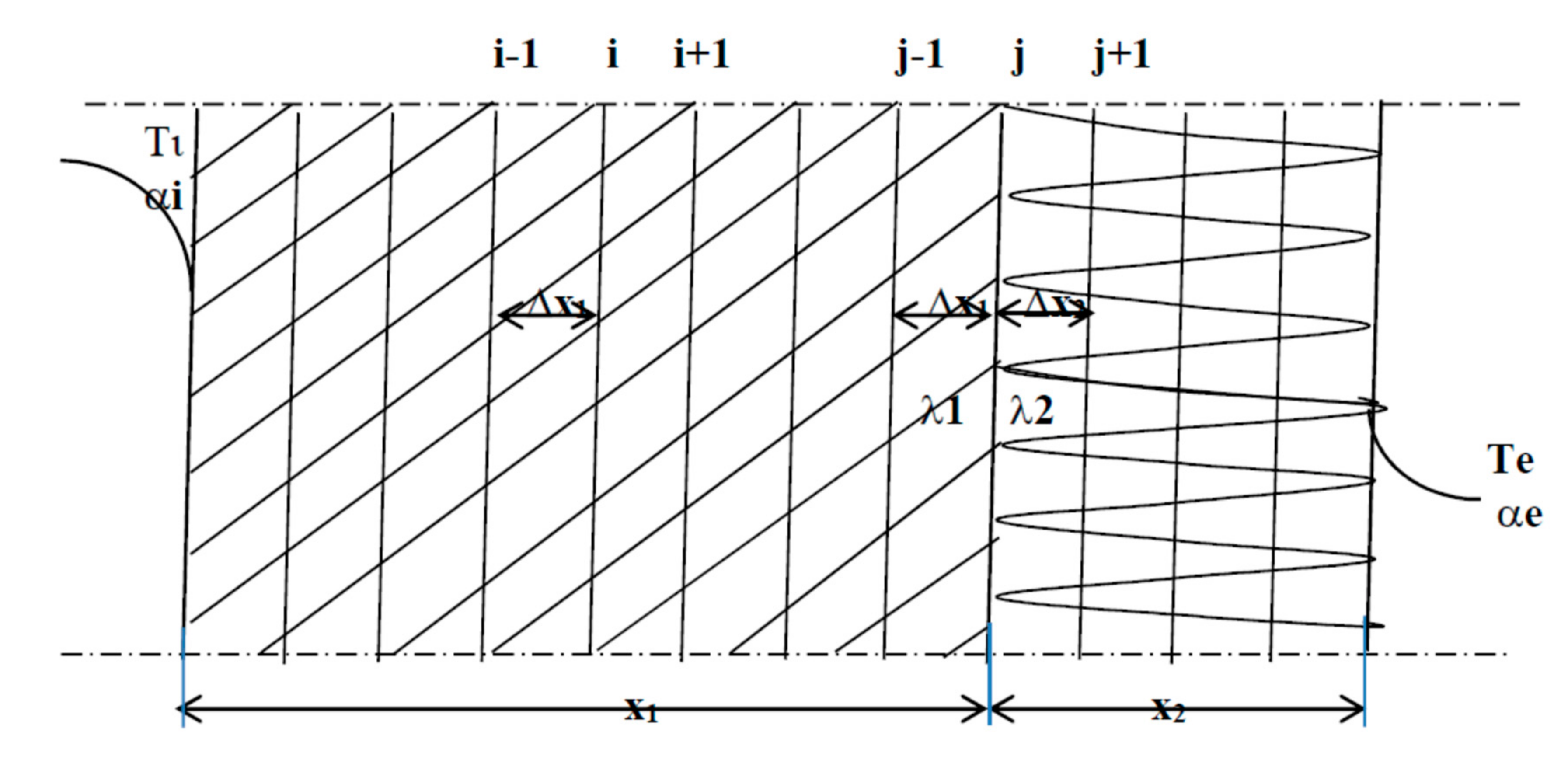
  • αi—coefficient of heat transfer from the wall surface to the internal air,
  • αe—heat transfer coefficient from the external wall surface to the outside air,
  • Asi—the surface of the outer wall inside the room,
  • Asw— the surface of the internal walls of the room,
  • Ase—the outer surface of the outer wall,
  • Af—reference surface (floors),
  • Ao—window area,
  • V—ventilation air stream,
  • qA—indicator of internal heat sources,
  • VVe—ventilation rate,
  • z—shading coefficient,
  • ws—radiation transmittance coefficient,
  • σs = 5.67 × 10⁻⁸ [W/m2K4]—radiation constant,
  • εsn—radiation absorption coefficient of the outer surface of the outer wall,
  • εs—radiation emission coefficient of the outer surface of the outer wall,
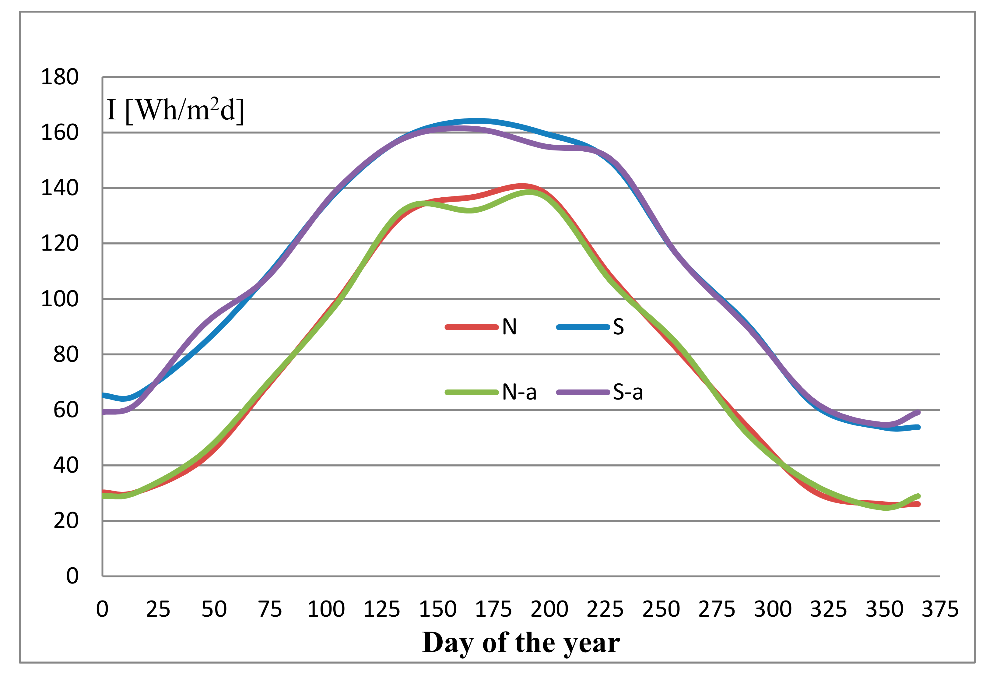
  • I—solar radiation intensity,
  • Ti—internal air temperature,
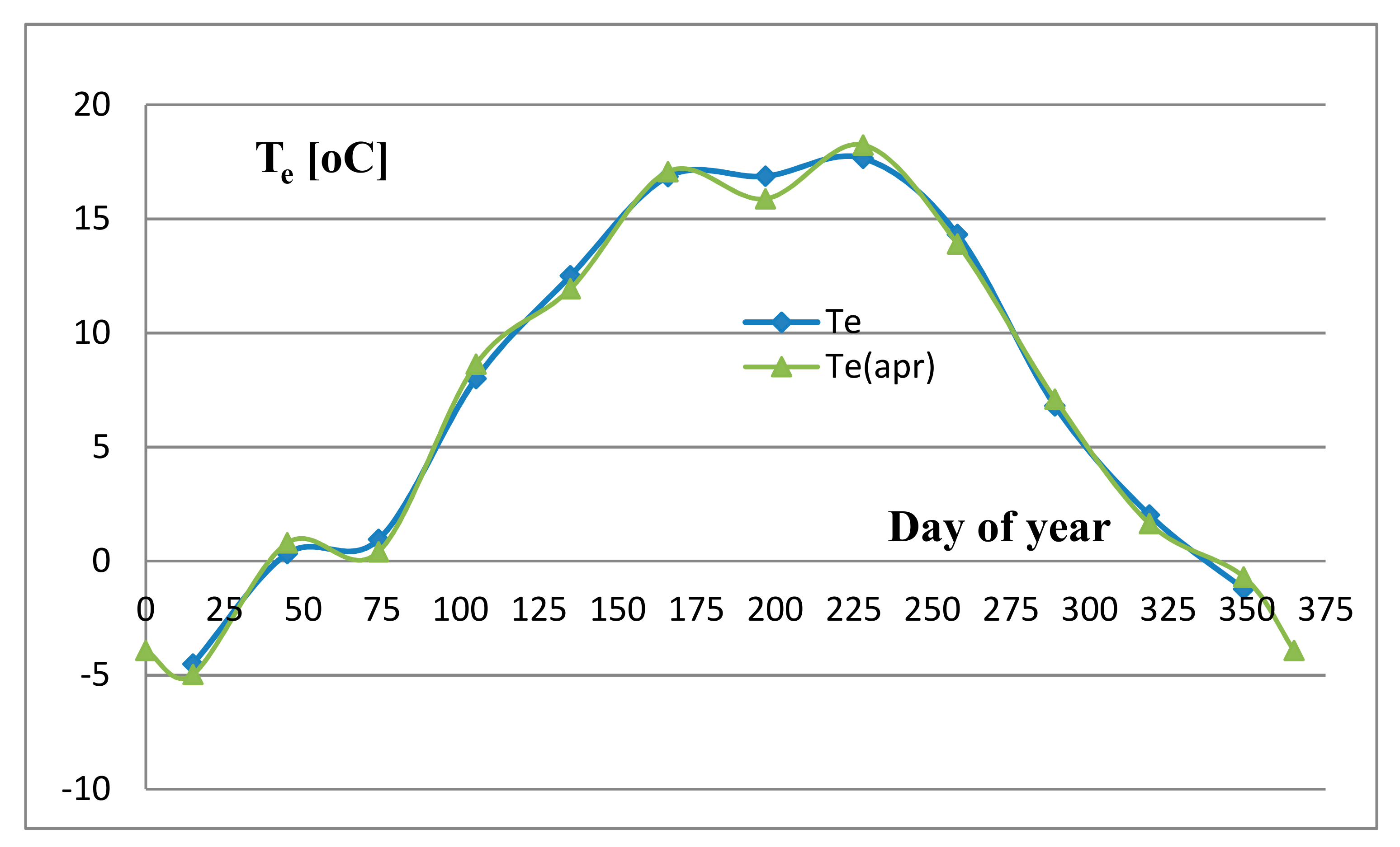
  • Te—outside air temperature,
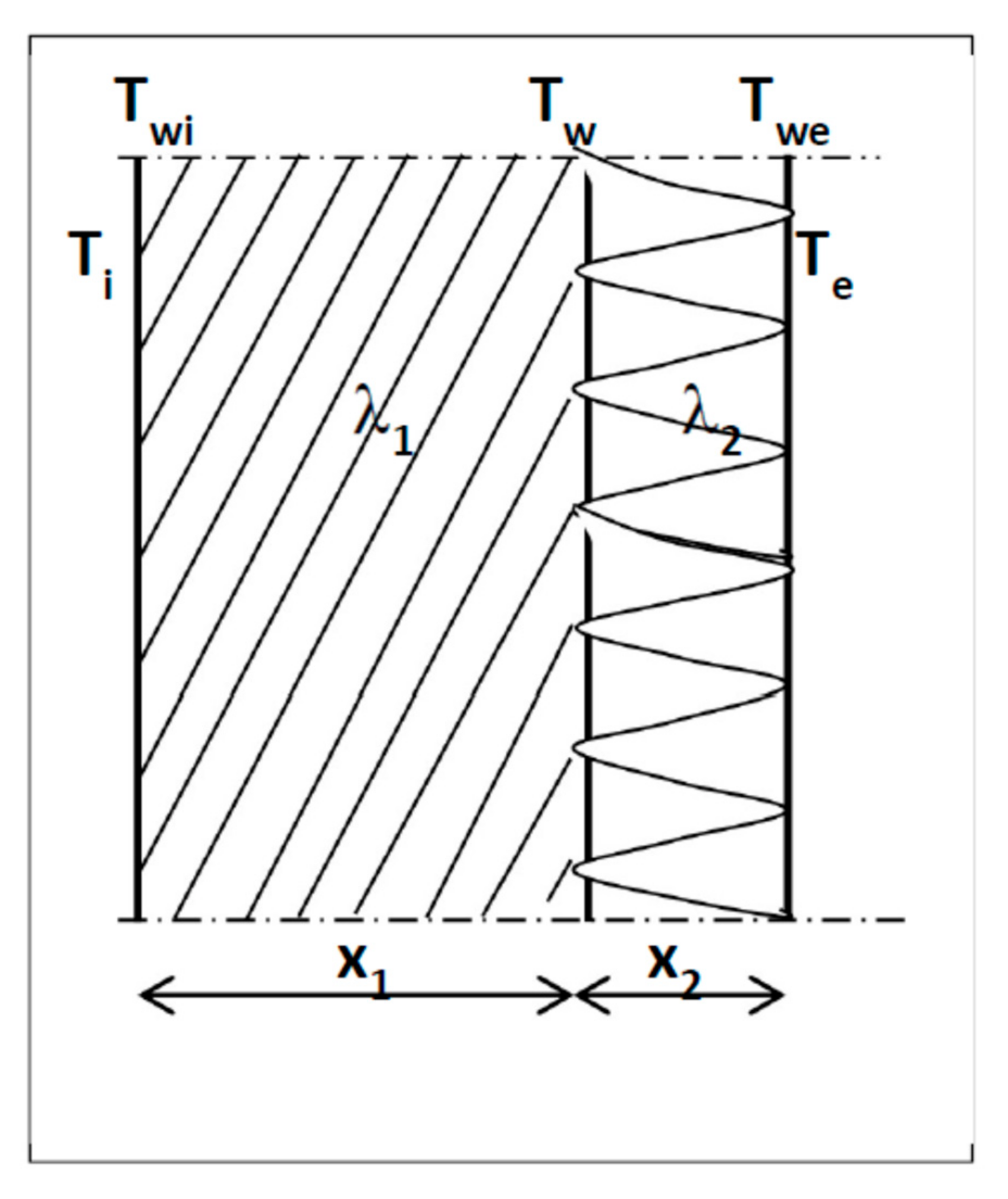
  • Twi—temperature of the inner surface of the outer wall,
  • Tsw—surface temperature of internal walls,
  • Twe—external wall surface temperature,
  • Tn—skyfall temperature.
Equation (2) shows the required heat output to heat the room during the heating season.
Q g = ( Q o + Q s i + Q V + Q s w ) ( Q o s + Q w )
The use of a heating device with the required thermal power and automatic temperature control results in maintaining the room temperature in accordance with the regulations [7].
In most cases, this temperature is taken as a constant value (Ti = const).
Outside the heating season, the heating devices are turned off (Qg = 0), and the internal air temperature is determined based on the thermal balance.
After using the thermal balance equations and transformations, the internal air temperature is described by the equation:
T i = z · w s · I · A o + q A · A f + ( U o · A o + V · ρ · c p ) · T e + α i · A s i   T w i + α i · A s w   T s w ( U o · A o + V · ρ · c p ) + α i · A s i + α i · A s w
Due to the variable temperature of the external air, outside the heating season also the temperature of the inside air is variable. The temperature of the inner surface of the walls is also variable.
This temperature is the result of heat transfer through the external wall between the room and the outside air.
With the simplifying assumption that the outside air temperature changes periodically according to the cosine function, the solution to the problem of heat conduction in a semi-infinite medium is described by the equations, according to [36,37]:
It was assumed that the air temperature changes according to the equation:
T f = T f o · c o s ( ω · t )
in which
ω = 2 · π t o
ν = ω 2 · π
where:
  • Tfo—amplitude of air temperature changes,
  • t—time,
  • ω—period of temperature changes,
  • to—change period time,
  • ν—frequency of changes,
The temperature T at depth x, below the surface, is described by the following dependencies:
T = C 2 · T f o · e ϖ 2 · a · · x · cos ( ω · t + ϖ 2 · a · x + C 2 )
C 1 = 1 1 + 2 · λ α · ω 2 · a + 2 · ( λ α · ω 2 · a ) 2
C 2 = a r c t g 1 1 + α λ · 2 · a ω
where:
  • λ—thermal conductivity,
  • a—thermal diffusivity of the area,
  • α—coefficient of heat transfer from air to the surface.
The constant C1 determines the degree of air temperature reduction resulting from the transfer of heat, while the constant C2 means the delay in wave propagation due to the transfer of heat to the surface.

3. Dynamics of Heat Transfer through an External Wall—Case Study

The external wall of the room is subjected to variable outside air temperature. Moreover, the external surface is influenced by the variable intensity of solar radiation. Climatic conditions cause periodic temperature variability in daily and annual cycles. Climate changes also cause changes in the temperature of external surfaces such as external building envelopes. Surface temperature changes are transferred deep into the material according to the principles of heat transfer. With a sufficient wall thickness, it can be treated as a semi-infinite medium for which the heat conduction problem has been analytically solved.
For example data:
  • Tfo = 20 °C,
  • a = 0.485 × 10⁻⁶ m2/s,
  • to = 24 h,
  • α = 12 W/(m2·K),
  • λ = 0.82 W/(m2·K).
The tendencies of temperature changes in the semi-infinite medium is shown in Figure 2. A negative coordinate x indicates temperature changes in the adjacent fluid.
The graphically presented temperature changes in the medium and equations [36,37] allow for the following conclusions:
  • There are temperature oscillations in the material with the same period in each plane, but with a phase shift in relation to the surface.
  • The amplitude of temperature changes on the surface is smaller than the amplitude of changes in air temperature (C1 < 1).
  • There is a phase shift in temperature changes (C2 < 0).
  • The amplitude of temperature changes in the material quickly decreases with depth.
  • The lower the frequency of temperature changes, the greater the amplitudes at the same depth.
The variability of temperature over time at different depths is shown in Figure 3. The presented considerations apply to a semi-infinite medium. However, they may be the basis for the analysis of temperature distribution in media with a finite, sufficiently large thickness. An example of such a medium are the external walls of a building, which is influenced by external air of variable temperature. There is a daily and annual periodicity of changes. Daily changes do not significantly affect the temperature distribution inside the wall under the surface, especially on the inner wall surface (from the room side). Annual changes, on the other hand, affect heat losses and, consequently, seasonal heat demand for heating.
In relation to the semi-infinite medium model, the following differences should be taken into account:
  • Changes in outside air temperature are periodic, but a description of the changes with a simple cosine function would be a simplification.
  • In addition to the transfer of heat between the outer surface and the air, there is a heat exchange by radiation (solar radiation).
  • The outer wall is usually multi-layered and therefore heterogeneous.
The periodic variability of outdoor air temperature and solar radiation intensity can be described by the Fourier series of the form [39]:
y = 1 2 a 0 + i = 1 k i · a i · c o s ( ω · t ) + i = 1 k i · b i · s i n ( ω · t )
The coefficients of the Fourier series should be determined on the basis of real data obtained, e.g., from measurements.
The temperature of the outside air and the intensity of solar radiation are climatic parameters and they are measured at meteorological stations. The results of long-term measurements are available on the website of the Ministry of Infrastructure [40].
For the selected weather station, we can read the average monthly and hourly average outside temperature values determined from multi-year measurements.
Using these values, data can be approximated by a Fourier series. For the Rzeszow-Jasionka meteorological station, the annual changes in the values of average daily outside air temperatures are shown in Figure 4, where the line resulting from the approximation of the data by the Fourier series (Te (apr)) is also plotted.
The parameters of the Fourier series for approximation calculations of the outside air temperature are presented in Table 1.
As can be seen from the diagram, there is a high agreement of the measurement data with the results obtained from the approximation equation. Significant differences occur in the summer, outside the heating season.
A similar procedure can be applied to record the variability of solar radiation, but due to the consideration of the external wall, only the radiation to the vertical plane will be important.
The Fourier series parameters for the approximation calculations of the radiation intensity per vertical surface (Wh/m2d) are summarized in Table 2.
Exemplary results for the Rzeszow-Jasionka actinometrical station are shown in Figure 5.
The comparison of the measurement results and those calculated from the Fourier series equation for the direction of the southern and northern radiation is presented in Figure 5.
Marking N in Figure 5 depicts the radiation changes from the North. Labeling S denotes imaging of changes in radiation from the southern side. Marking N-a represents the results of approximation of radiation changes from the North using the Fourier series. Then, by analogy, S-a refers to the results of the approximation of radiation changes from the south side.
Remarks on the compliance of the approximation with the data are the same as in the case of the approximation of the outside air temperature.
Increasing the accuracy of the approximation is possible by increasing the amount of Fourier series components. For the assumed purpose of the analysis of the temperature distribution in the external wall, the assumed accuracy is sufficient.

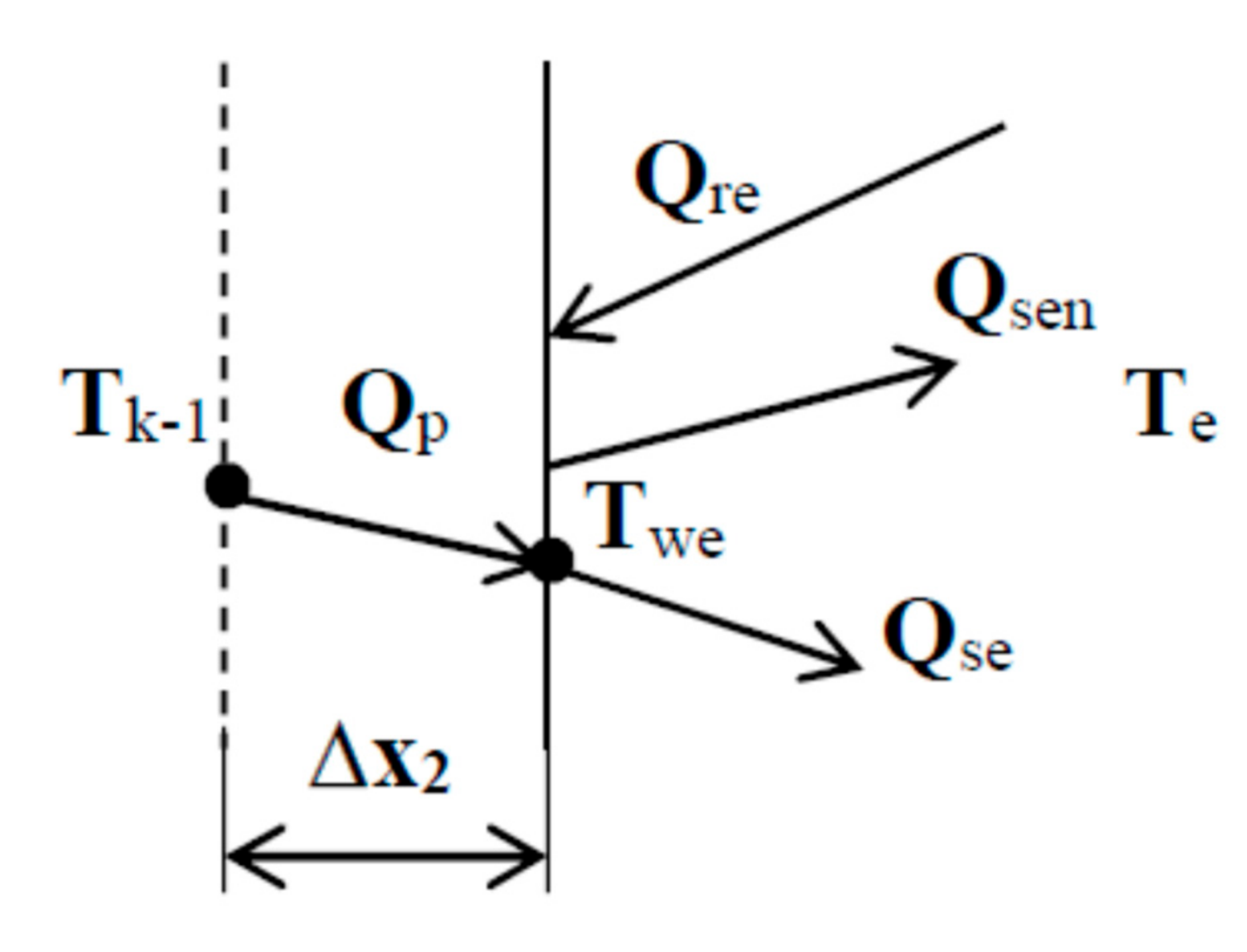
4. Heat Losses through the External Wall—Case Study

The external wall separates the outside environment and the interior of the room. Such a wall is subjected to an externally variable air temperature as well as solar radiation. Climatic conditions cause periodic temperature variability as well as the variability of radiation intensity, and these changes occur in daily and annual periods. The resulting wall temperature distribution makes it difficult to provide a strict analytical solution, especially in the case of a multi-layer partition.
Simplified methods can be used to solve special cases, e.g., the finite difference method (MRS).
The analysis of heat loss through the external partition is made below, with the following assumptions.
On the side of the inner wall (in the room), the air temperature remains constant. This is the case during the heating season with automatic temperature control (thermostatic valves).
The heat transfer from the inside air to the surface takes place by transfer, with a transfer factor taking into account the radiation.
On the outer side of the outer wall, heat is transferred to the outside air by taking over.
On the outer side of the outer wall, heat transfer also takes place through radiation to the outer space (the sky).
The outside air temperature changes throughout the year according to the climatic conditions.
Solar radiation falls on the outer surface of the wall with periodic, annual variability.
The values of external temperature and radiation intensity were taken as daily averages.
The image of the partition in question, with significant values marked, is shown in Figure 6.
The variable temperature distribution in the wall was determined by the finite difference method based on heat transfer equations, taking into account the thermal balance of the room.
Due to the variable temperature of the outside air, the temperature of the inside surface of the outside walls is also variable.
This temperature is the result of heat transfer through the external wall between the room and the outside.
When applying the finite difference method (FDM) to solve the transient heat conduction in the outer wall, formulas based on the calculation scheme are obtained (Figure 7).
The formulas resulting from the discretization of areas were used for the calculations.
Inner surface temperature of outer wall:
T w i = T i + λ i α i · Δ x 1 · T 1 1 + λ i α i · Δ x 1
Surface temperature at the boundary of the layers:
T w = λ 1 Δ x 1 · T j 1 + λ 2 Δ x 2 · T j + 1 λ 1 Δ x 1 + λ 2 Δ x 2
The temperature of the outer surface of the outer wall was determined from the balance sheet (Figure 8):
Q p + Q r e = Q s e + Q s e n
Taking into account the Equations (10)–(12) and the heat conduction equation under the surface of the partition (24), it can be concluded that:
Q p = λ 2 Δ x 2 · A s e · ( T k 1 T w e )
After substitution and transformations, the temperature of the outer surface of the outer wall is described by the relationship:
T w e = ε s · I + λ 2 Δ x 2 · T k 1 + α e · T e ε n · ( T w e 4 T n 4 ) α e + λ 2 Δ x 2
Due to the presence of Twe, the equation is solved by the iteration method.
Signs:
  • Tn—skyfall temperature
  • σs = 5.67 × 10⁻⁸ [W/m2K4]—radiation constant
  • εs—surface radiation absorption coefficient
  • εsn—surface radiation emission coefficient
  • αe—heat transfer coefficient from the external wall surface to the outside air
  • λ2—thermal conductivity coefficient of the insulating layer
  • Δx2—step of discretization of the insulating layer
The above equations are completed with boundary conditions.
  • The heating season was assumed to occur during the period when the outside air temperature is lower than 12 °C (Te < 12 °C).
  • If, during the heating season, the heat losses are greater than the heat gains, the heating control system maintains a constant internal temperature (Ti = Tio).
  • If in the heating season the heat losses are lower than the heat gains, the control system switches the heating off and the internal temperature results from the thermal balance.
  • Outside the heating season, the internal temperature results from the thermal balance.

5. Results and Discussion

5.1. Assumptions and Output Parameters

Using the previously given equations, calculations of the parameters of the room and the external partition were made for variable external conditions [41].
The calculations were made for several variants of rooms with general assumptions:
  • A living room.
  • The heat transfer coefficient on the inside and outside is constant in accordance with the standard [42].
  • Natural ventilation with the intensity resulting from meeting the requirements of the standard [43].
  • The thermal conductivity coefficient of the wall construction material and insulation is constant.
  • Internal heat gains are constant.
Data for calculations, with values (according to [43]):
  • qA = 6.8 W/m2—single-family buildings,
  • qA = 7.0 W/m2—multi-family buildings,
  • VVe = 0.31 × 10⁻³ m3/(sm2)—single-family buildings,
  • VVe = 0.32 × 10⁻³ m3/(sm2)—multi-family buildings.
Relationship between VVe coefficient and the number of exchanges n:
n = 3.6 · V V e h
  • h—room height.
Thermal conductivity:
  • λ1 = 0.82 W/mK (brick wall),
  • λ2 = 0.032 W/mK (polystyrene insulation).
Room dimensions:
  • a = 3.0 m—the width of the room,
  • b = 4.0 m—room depth,
  • h = 3.0 m—room height,
  • Ao = 1.96 m2—window area.
Meteorological data:
Sample calculations were made using the meteorological data for the Rzeszów-Jasionka measuring station.
The table of hourly changes in outside temperature and changes in the intensity of solar radiation was used, provided by the website of the Ministry of Infrastructure [40].
The example assumes the location of the outer wall towards the north.
It is assumed that the final result of the calculations will be the determination of the variability of the heat demand for space heating over the year, taking into account the variability of climatic conditions and the inertia of building partitions.
The basis for determining the heat demand is Equation (2). The components of the equation were determined by Equations (3)–(10) using the assumptions made above.
The calculations were made for a living room with an external wall made of brick, 50-cm thick, for the cases: without insulation and with insulation with a layer of polystyrene 5-, 10-, 15-, 20-, and 25-cm thick. The results of the calculations are presented in the following charts.

5.2. Calculation of Indoor Air Temperature

In the heating season, the heat losses exceed the heat gains in the room, which are supplemented by the heating system. The regulation of this system allows for the maintenance of the constant temperature Ti = 20 °C, assumed in the example. In summer, the temperature of the indoor air is the result of the heat balance of gains and losses. Temperature fluctuations increase as the thickness of the insulation increases.
The calculation results of the average daily temperature of indoor air obtained using the Equation (14) are presented graphically in Figure 9.
During the heating season, the regulation ensures a constant temperature. In summer, there is a temperature change, and these fluctuations increase with increasing insulation thickness. The labels in Figure 9 and Figure 10 were signed by adding units of insulation thickness as “Ti-0 cm” and analogously “Twi-0 cm”.
From the graph in Figure 9 you can read the time during which heating is required, i.e., the duration of the heating season. This time depends on the insulation of the outer wall (insulation thickness).

5.3. Calculation of the Surface Temperature of the Inner Outer Wall

The temperature of the inner surface of the outer wall is the result of heat conduction through the wall and taking heat from the inner air. It clearly depends on the wall insulation. It was calculated according to the Equation (22) and the results are presented in Figure 10. This temperature and its fluctuations throughout the year clearly depend on the wall insulation.
The annual amplitude of changes in this temperature decreases with increasing insulation thickness. In the absence of insulation, the lowest temperatures appear around the beginning of March, and for an insulated wallm around mid-April.
Fluctuations in the average daily temperature ΔTi (Figure 11) with efficient regulation in the heating season are very small during the year (<0.51 °C) and depend to a small extent on the wall insulation. On the other hand, the temperature fluctuations of the inner surface of the outer wall Twi depend on the insulation. For a wall without insulation, the maximum difference in a year is 3.14 °C. The difference in temperature values when changing the insulation thickness from 5 to 25 cm, equal to 0.49–0.86, is small and it has little effect on thermal comfort.

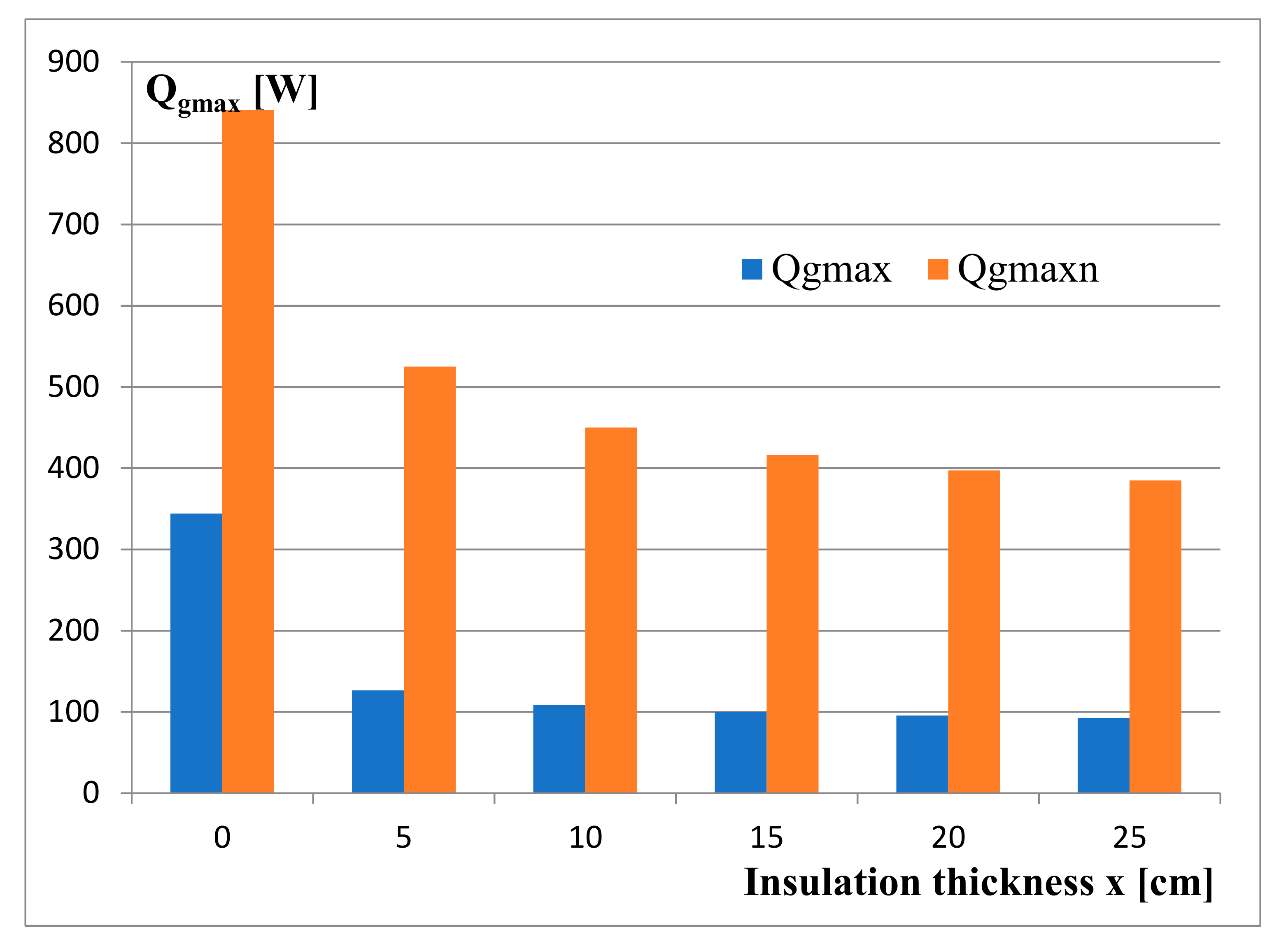
5.4. Analysis of Thermal Power Variability for Heating Purposes

Using the proposed methodology, calculations of thermal power for heating were performed for the conditions assumed in Section 2. The diagram given in Figure 12 shows the dependence of this power on the insulation thickness.
The chart of changes in heat demand for heating (Figure 11) clearly shows the division into the heating season and the summer season. The demand in the heating season depends (which is obvious) on the insulation of the outer wall. The length of the heating season tg also depends on the insulation performance.
The maximum heat output, which is the basis for the selection of heating devices, is also different for each case. The comparison of these powers is shown in Figure 13. The diagram also includes heating powers Qmaxn calculated on the basis of the applicable standards. Qmax denotes the maximum thermal power for a given case of the partition structure, calculated according to the considered methodology. Qmaxn means the maximum thermal power for a given case of the partition structure, calculated on the basis of the applicable standard PN EN 12831 titled “Heating installations in buildings. Design heat load calculation method”.
Among the calculated thermal powers presented in Figure 12, the maximum powers Qgmax necessary to ensure thermal comfort were selected. Such powers Qgmaxn were also calculated for the considered cases in accordance with the standard. The values are presented in the Table 3 and in the diagram in Figure 13.
The following conclusions can be drawn from the presented values:
  • Taking into account the thermal inertia of the partitions makes it possible to perform a significant reduction in the demand for thermal power, and thus the use of smaller devices.
  • For the considered partition, the calculated thermal power determined by the adopted method is only about 40% of the value calculated according to the standard.
  • The reduction in thermal power depends on the thermal inertia of the partitions.
  • Due to the low thermal capacity, the insulation thickness has a little effect on the maximum heat output.

5.5. The Dependence of the Time of the Heating Season on the Thickness of the Insulation

The dependence of the length of the heating season on the insulation thickness is shown in Figure 14.
The diagram in Figure 14 clearly shows the dependence of the heating season on the “insulation” of external walls. Increasing the thickness of the insulation shortens the heating season, which contributes to reducing the annual heat consumption for heating purposes. For comparison, the graph also shows (red) the time determined on the basis of the annual variability of the outside air temperature. This time is approximately in line with the calculation method adopted for the wall without external insulation (x = 0). This confirms the correctness of the adopted calculation methodology and the correctness of the performed calculations.

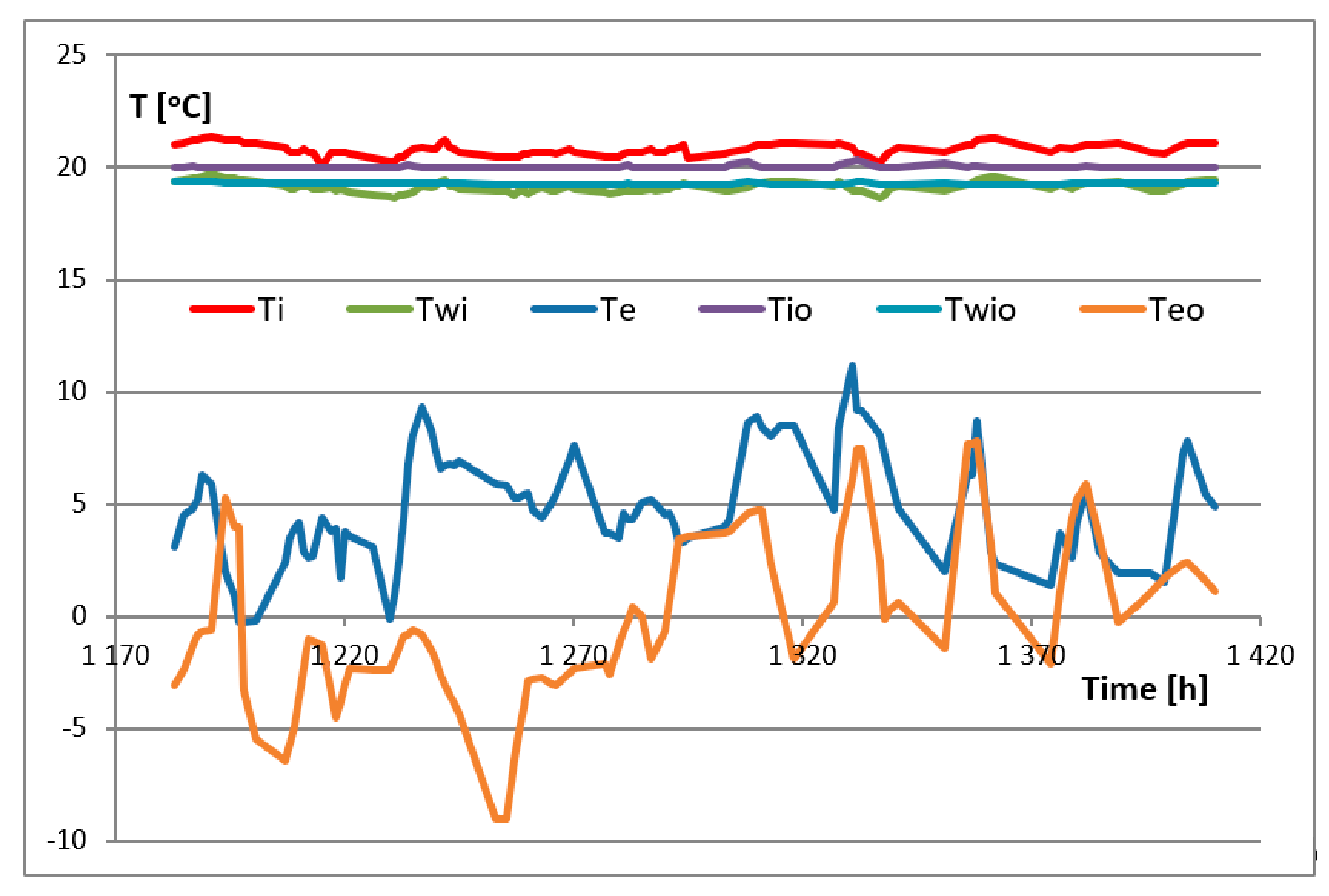
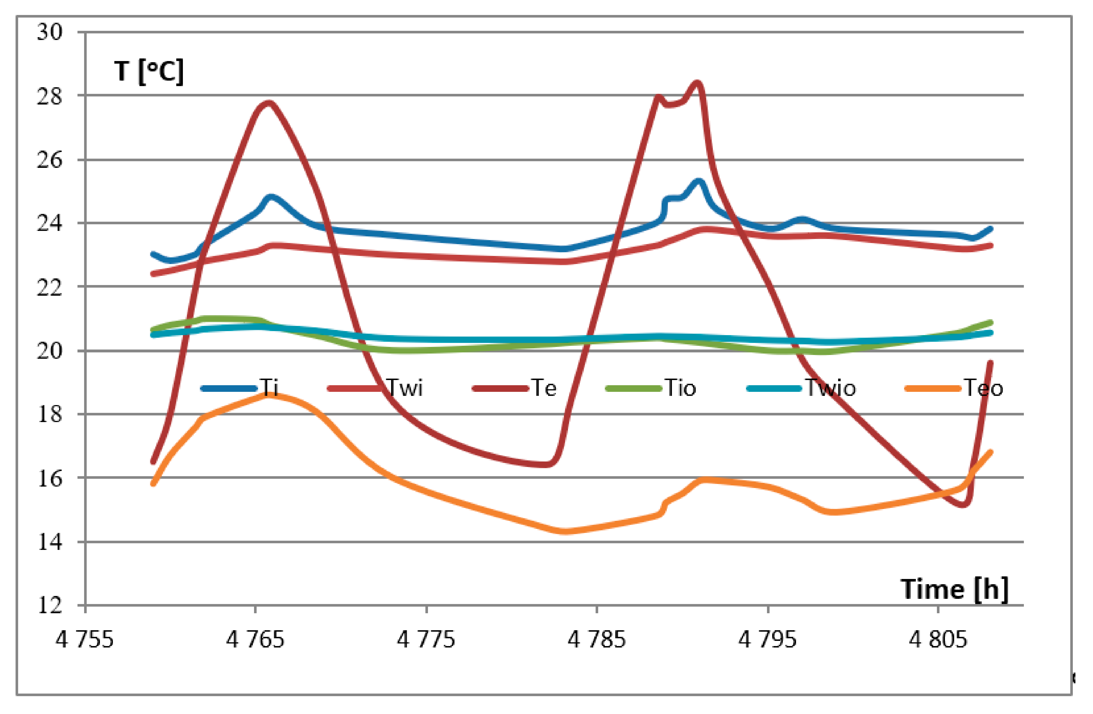
5.6. Validation of the Model by Using Fragmented Temperature Measurements

In order to assess the compliance of the adopted calculation methodology with the actual conditions, fragmentary temperature measurements were performed. Measurements were made in a real facility in a single-family residential building, on an external brick wall with the following parameters:
  • Wall thickness: 50 cm,
  • Thickness of the outer polystyrene insulation: 10 cm
  • Thermal conductivity of the wall: λ = 0.82 W/(m·K)
  • Thermal conductivity of the insulation: λ= 0.032 W/(m·K)
Following temperatures measurements were taken:
  • Ti—internal air temperature
  • Twi—temperature of the inner surface of the outer wall
  • Te—outside air temperature
The purpose of the measurements is to show the effect of thermal inertia of the partitions on the changes in internal temperature. The measure of the influence of inertia is the amplitude of changes in the internal temperature and the temperature of the internal surface of the external partition as a function of the amplitude of changes in the external air temperature.
Measurements were taken continuously and the values were averaged over an hourly period for analysis.
This impact was initially analyzed on the basis of measurements conducted from 20–29 February 2020 and from 18–20 July 2020. The results presented in the table below were obtained for these cases. Results of calculations and measurements have been presented in Table 4.
Exemplary results for several hours in the heating season (February) are shown in Figure 15 as a function of successive hours throughout the year. The graph also shows the corresponding temperatures for these hours obtained from calculations (Tio, Twio, Teo).
On the horizontal axes of the graphs (Figure 15 and following), the time is defined as successive hours of the year. Such a system was adopted for the purpose of comparing the results of measurements and calculations, because the calculations used climatic data for the following hours of the year. The hours for calculations and measurements were kept consistent.
Supplementary markings:
  • Ti—measured internal air temperature
  • Te—measured outside air temperature
  • Twi—measured temperature of the inner surface of the outer wall
  • Tio—internal air temperature adopted for calculations
  • Teo—outside air temperature taken for calculations
  • Twio—calculated temperature of the inner surface of the outer wall
During the heating season with variable outside air temperature, there are small changes in the temperature of the inner surface of the outer wall. The temperature value is comparable with the value calculated according to the adopted method.
In the summer, we can observe a similar tendency. A detailed comparison will be the purpose of further research. We initially present sample measurement results for summer season. We presented obtained results of researches in the Figure 16.
In order to verify the correctness of the adopted methodology, the amplitudes of differences in temperature between the internal air and the internal surface of the external wall were determined and presented in the Table 5.
During the measurement period, there were significant fluctuations in the outside temperature and due to this there were also changes in the internal temperature, despite the regulation of the heating with a thermostatic valve. For this reason, there was a change in the temperature difference between the inside air and the wall surface. The course of amplitude changes during the period from 20 to 29 February 2020 is shown in Figure 17.
Analogically, the course of amplitude changes during the time from 18 to 20 July 2020 is presented in Figure 18.
In order to verify the correctness of the adopted methodology, additional, more precise temperature measurements were made for the period from 9 to 17 November 2020. The measurement results are shown in Figure 19 and Figure 20.
The measurement results were compared with the values used in the calculations in the adopted model and are presented in Table 6.
The influence of the thermal inertia of partitions on changes in internal temperature was analyzed. The results of measurements and calculations are shown in Figure 20.
Changes in the temperature of the outside air cause slight changes in the temperature of the inside surface of the outside wall. The value of the wall surface temperature is comparable with the value calculated in accordance with the adopted method, which is shown in Figure 20.
In order to better visualize the compliance of the measurement results with the calculations, relative deviations calculated on the basis of the differences in the measurement and calculation results were determined. The deviations were applied to the temperature of the inner surface of the outer wall, because this temperature determines the transfer of heat for all three analyzed measurement series.
δ = 100 · T w i T w i o T w i   [ % ]
when:
  • δ—relative deviation of the measured and calculated internal surface temperature.
The changes of the relative deviations of the values measured for the period from 9 to 17 November 2020 is shown in Figure 21. The relative deviations for all three measurement series are presented in Table 7.
A small value of the average deviation of the measurement and calculation results during the heating season indicates the correctness of the adopted analysis method. The big difference in July is caused by very large changes in outside air temperatures, deviating from typical meteorological years. It should be emphasized that such a result is obtained from measurements of a real object (not in a laboratory) under very variable climatic conditions. Moreover, the temperature of the indoor air in the summer with no air conditioning is directly related to the temperature of the outdoor air and is not regulated.
Furthermore, complete measurements are planned to fully assess the compliance of the calculation model.
The presented data show the following conclusions:
  • In the winter period (February), the measured amplitude of changes in the outside temperature of 11.50 °C corresponds to the amplitude of changes in the internal temperature of 1.30 °C and the amplitude of changes in the temperature of the inside surface of the external wall, which equals 1.00 °C.
  • Similar relations exist for the period from 18 to 20 July 2020.
  • In any case, the average amplitude of changes in the temperature of the internal surface of the external wall is smaller than the amplitude of changes in the temperature of internal air.
  • The same conclusion follows from the calculation results. Quantitative differences are caused by the random selection of the measurement period and the uniqueness of the climate parameters.
  • Reducing the amplitude has a positive effect on maintaining thermal comfort.

6. Summary and Conclusions

The current regulations define the rules for calculating the heat demand for heating based on the difference between the maximum and minimum outside air temperature for the climate zone. The calculations do not take into account the thermal inertia of building partitions.
The main aim of the article is to determine the influence of the thermal inertia of building partitions on the building’s heating system, taking into account changing climatic conditions.
The process of heat transfer through the partitions is described in the literature, and the novelty in this respect is the use of boundary conditions appropriate for the nature of the partition, i.e., variable outside air temperature and solar radiation intensity. These conditions are taken into account in the literature—also in standards—, but in a simplified way through indicators covering longer periods (usually monthly). This variability is not considered when constructing an ordered diagram of heat loads, which affects the determination of the heating season time.
The thermal power of heating devices is assumed on the basis of calculations made for the steady state with extreme parameters, without taking into account the thermal inertia. In the presented study, the influence of the thermal inertia of the external building partition on the heat exchange between the building’s interior and its surroundings was analyzed. Different thicknesses of the insulation of the outer partition were considered. The ongoing dynamic processes were analyzed computationally using the finite difference method (FDM).
Based on the obtained calculation and measurement results, the following conclusions can be drawn:
  • Maximum power for heating, determining the selection of heating devices, is lower than the values determined according to the applicable calculation rules. The difference between the thermal power calculated on the basis of the applicable PN EN 12831 standard and the maximum power for a given case of the partition structure, calculated in accordance with the considered methodology presented in the article, decreases with increasing insulation thickness and equals from 41% to 24%.
  • The reduction in heat output depends on the thickness of the insulation, but to a much lesser extent than the increase in thickness. The economic correlation between these values requires further analysis.
  • The duration of the heating season is also dependent on the insulation of external partitions and it is definitely shorter than that determined on the basis of changes in external temperature.
  • With the efficient regulation of the internal temperature in the heating season, the insulation of the external partition allows for very small temperature fluctuations of the internal surface of the partitions, which has a positive effect on the thermal comfort of the rooms.
  • The results of the research on temperature variability over time presented in the article confirm the fact that the temperature fluctuations of the surface of the partitions, which reflect the heat transfer from the internal air to the partition surface, and the heat conduction inside the partition and heat transfer from the partition to the outside air are much less variable than the fluctuations of outdoor and indoor temperatures. With the amplitude of changes in the outside air temperature in summer amounting to 11.5 °C, the amplitude of changes in the internal temperature of the surface of the analyzed external wall is 1.00 °C, while the amplitude of changes in the internal temperature is 1.30 °C. In winter, these fluctuations demonstrate similar relationships with greater differences.
  • The performed research confirms the compliance of the adopted model of heat transfer dynamics testing. Average temperature deviations measured and calculated in the winter season range from −0.85% to +0.45%. A significant deviation in the summer season is due to the lack of temperature regulation.
The development of issues related to the dynamics of heat transfer, taking into account the variability of weather conditions and thermal inertia in buildings, will be the subject of future research conducted by the authors of this article.

Author Contributions

Conceptualization, W.S. and B.B., methodology, W.S. and B.B; writing—original draft preparation, B.B. and W.S.; writing—review and editing, B.B. and W.S. All authors have read and agreed to the published version of the manuscript.

Funding

This research received no external funding.

Conflicts of Interest

The authors declare no conflict of interest.

References and Notes

  1. Directive 2002/91/EC of the European Parliament and of the Council of 16 December 2002 on the Energy Performance of Buildings. Official Journal of the European Union, L 1/65.
  2. Directive 2010/31/EU of the European Parliament and of the Council of 19 May 2010 on the Energy Performance of Buildings (Recast). Official Journal of the European Union, L 153/13.
  3. Directive 2012/27/EU of the European Parliament and of the Council of 25 October 2012 on Energy Efficiency, Amending Directives 2009/125/EC and 2010/30/EU and Repealing Directives 2004/8/EC and 2006/32/EC. Official Journal of the European Union, L 315/1.
  4. The Act of 20 May 2016 on energy efficiency (Journal of Laws of 2016, item 831), as amended.
  5. The Act of 29 August 2014 on the energy performance of buildings (Journal of Laws of 2014, item 1200), as amended.
  6. Directive (EU) 2018/844 of the European Parliament and of the Council of 30 May 2018 Amending Directive 2010/31/EU on the Energy Performance of Buildings and Directive 2012/27/EU on Energy Efficiency. Official Journal of the European, L 156/75.
  7. Regulation of the Minister of Infrastructure of 12 April 2002 on Technical Conditions to be Met by Buildings and Their Location (Journal of Laws No. 75, item 690), as amended.
  8. Regulation of the Minister of Infrastructure of 27 February 2015 on the Methodology for Determining the Energy Performance of a Building or Part of a Building and Energy Performance Certificates (Journal of Laws of 2015, item 376).
  9. Satchwell, A.J.; Cappers, P.A.; Deason, J.; Forrester, S.P.; Frick, N.M.; Gerke, B.F.; Piette, M.A. A Conceptual Framework to Describe Energy Efficiency and Demand Response Interactions. Energies 2020, 13, 4336. [Google Scholar] [CrossRef]
  10. Babiarz, B. Aspects of heat supply security management using elements of decision theory. Energies 2018, 11, 2764. [Google Scholar] [CrossRef] [Green Version]
  11. Cholewa, T.; Życzyńska, A. Experimental evaluation of calculated energy savings in schools. J. Therm. Anal. Calorim. 2020, 1–8. [Google Scholar] [CrossRef]
  12. Babiarz, B. Heat supply system reliability management. Safety and reliability: Methodology and Applications. In Proceedings of the European Safety and Reliability Conference, ESREL 2014, Wroclaw, Poland, 14–18 September 2014; Taylor & Francis Group: London, UK, 2015; pp. 1501–1506. [Google Scholar]
  13. Cholewa, T.; Balaras, C.A.; Nižetić, S.; Siuta-Olcha, A. On calculated and actual energy savings from thermal building renovations—Long term field evaluation of multifamily buildings. Energy Build. 2020, 223, 110145. [Google Scholar] [CrossRef]
  14. Babiarz, B.; Kut, P. District heating simulation in the aspect of heat supply safety. In Proceedings of the VI International Conference of Science and Technology INFRAEKO 2018 Modern Cities. Infrastructure and Environment, Cracov, Poland, 7–8 June 2018. [Google Scholar] [CrossRef] [Green Version]
  15. Chicherin, S.; Mašatin, V.; Siirde, A.; Volkova, A. Method for Assessing Heat Loss in A District Heating Network with A Focus on the State of Insulation and Actual Demand for Useful Energy. Energies 2020, 13, 4505. [Google Scholar] [CrossRef]
  16. Basinska, M.; Koczyk, H.; Szczechowiak, E. Sensitivity analysis in determining the optimum energy for residential buildings in Polish conditions. Energy Build. 2015, 107, 307–318. [Google Scholar] [CrossRef]
  17. Rim, M.; Sung, U.J.; Kim, T. Application of Thermal Labyrinth System to Reduce Heating and Cooling Energy Consumption. Energies 2018, 11, 2762. [Google Scholar] [CrossRef] [Green Version]
  18. Dec, E.; Babiarz, B.; Sekret, R. Analysis of temperature, air humidity and wind conditions for the needs of outdoor thermal comfort. In Proceedings of the 10th Conference on Interdisciplinary Problems in Environmental Protection and Engineering EKO-DOK 2018 E3S Web of Conferences 44, Dolny Śląsk, Poland, 8–10 April 2019. [Google Scholar] [CrossRef] [Green Version]
  19. Krawczyk, D.A.; Wądołowska, B. Analysis of indoor air parameters in an education building. Energy Procedia 2018, 147, 96–103. [Google Scholar] [CrossRef]
  20. Oldewurtel, F.; Sturzenegger, D.; Morari, M. Importance of occupancy information for building climate control. Appl. Energy 2013, 101, 521–532. [Google Scholar] [CrossRef]
  21. Korkas, C.D.; Baldi, S.; Michailidis, I.; Kosmatopoulos, E.B. Occupancy-based demand response and thermal comfort optimization in microgrids with renewable energy sources and energy storage. Appl. Energy 2016, 163, 93–104. [Google Scholar] [CrossRef]
  22. Xue, Y.; Ge, Z.; Du, X.; Yang, L. On the Heat Transfer Enhancement of Plate Fin Heat Exchanger. Energies 2018, 11, 1398. [Google Scholar] [CrossRef] [Green Version]
  23. Emmel, M.G.; Abadie, M.O.; Mendes, N. New external convective heat transfer coefficient correlations for isolated low-rise buildings. Energy Build. 2007, 39, 335–342. [Google Scholar] [CrossRef]
  24. Dylewski, R. Optimal Thermal Insulation Thicknesses of External Walls Based on Economic and Ecological Heating Cost. Energies 2019, 12, 3415. [Google Scholar] [CrossRef] [Green Version]
  25. Krasoń, J.; Miąsik, P.; Lichołai, L.; Dębska, B.; Starakiewicz, A. Analysis of the Thermal Characteristics of a Composite Ceramic Product Filled with Phase Change Material. Buildings 2019, 9, 217. [Google Scholar] [CrossRef] [Green Version]
  26. Kim, D.; Cox, S.J.; Cho, H.; Yoon, J. Comparative investigation on building energy performance of double skin façade (DSF) with interior or exterior slat blinds. J. Build. Eng. 2018, 20. [Google Scholar] [CrossRef]
  27. Wilson, M.; Luck, R.; Mago, P.J.; Cho, H. Building Energy Management Using Increased Thermal Capacitance and Thermal Storage Management. Buildings 2018, 8, 86. [Google Scholar] [CrossRef] [Green Version]
  28. Zheng, X.; Heshmati, A. An Analysis of Energy Use Efficiency in China by Applying Stochastic Frontier Panel Data Models. Energies 2020, 13, 1892. [Google Scholar] [CrossRef]
  29. Seo, B.; Yoon, Y.B.; Yu, B.H.; Cho, S.; Lee, K.H. Comparative Analysis of Cooling Energy Performance Between Water-Cooled VRF and Conventional AHU Systems in a Commercial Building. Appl. Therm. Eng. 2020, 170, 114992. [Google Scholar] [CrossRef]
  30. Kim, C.-H.; Lee, S.-E.; Lee, K.H.; Kim, K.-S. Detailed Comparison of the Operational Characteristics of Energy-conserving HVAC Systems during the Cooling Season. Energies 2019, 12, 4160. [Google Scholar] [CrossRef] [Green Version]
  31. Wetter, M. Modelica-based modelling and simulation to support research and development in building energy and control systems. J. Build. Perform. Simul. 2009, 2. [Google Scholar] [CrossRef] [Green Version]
  32. Manz, H.; Frank, T.h. Thermal simulation of buildings with double-skin façades. Energy Build. 2005, 37. [Google Scholar] [CrossRef]
  33. Clarke, J.A. Energy Simulation in Building Design; Butterworth-Heinemann: Oxford, UK, 2001. [Google Scholar]
  34. Gerlich, V. Modelling of Heat Transfer in Buildings. In Proceedings of the 25th Conference on Modelling and Simulation, Krakow, Poland, 7–10 June 2011. [Google Scholar] [CrossRef] [Green Version]
  35. Simões, N.; Prata, J.; Tadeu, A. 3D Dynamic Simulation of Heat Conduction through a Building Corner Using a BEM Model in the Frequency Domain. Energies 2019, 12, 4595. [Google Scholar] [CrossRef] [Green Version]
  36. Madejski, J. Theory of Heat Transfer; Szczecin University of Technology: Szczecin, Poland, 1998. (In Polish) [Google Scholar]
  37. Staniszewski, B. Heat transfer. In Theoretical Basics; PWN: Warsaw, Poland, 1979. [Google Scholar]
  38. Szymański, W. Heat transfer. Fundamentals, Federation of Scientific and Technical Associations Council in Rzeszów, Rzeszów 2019 (In Polish).
  39. Bronsztejn, I.N.; Siemiendiajew, K.A. Maths. In Encyclopedic Guide; PWN: Warsaw, Poland, 1968. [Google Scholar]
  40. Typical Meteorological Years and Statistical Climatic Data for Energy Calculations of Buildings. Available online: www.mib.gov.pl (accessed on 15 September 2020).
  41. PN-EN ISO 52016-1: 2017 Energy performance of buildings—Energy needs for heating and cooling, internal temperatures and sensible and latent heat loads—Part 1: Calculation procedures (ISO 52016-1:2017).
  42. PN-EN-ISO 6946: Building components and building elements. Thermal resistance and heat transfer coefficients. Calculation Method.
  43. PN-83/B-03430 Ventilation in residential buildings, collective residence and public utility buildings. Requirements.
Figure 1. Balance sheet diagram.
Energies 13 06469 g001
Figure 2. Temperature changes along the depth in a semi-infinite medium [38].
Energies 13 06469 g002
Figure 3. An example of temperature changes with time at depth x in a semi-infinite medium [38].
Energies 13 06469 g003
Figure 4. Annual variability of outside air temperature for Rzeszow city.
Energies 13 06469 g004
Figure 5. Comparison of the annual variability of the intensity of solar radiation measured and from the approximation equation for Rzeszow city.
Energies 13 06469 g005
Figure 6. Cross-section through the outer wall.
Energies 13 06469 g006
Figure 7. Calculation scheme.
Energies 13 06469 g007
Figure 8. Balance diagram of the external surface.
Energies 13 06469 g008
Figure 9. Indoor air temperature.
Energies 13 06469 g009
Figure 10. The temperature of the inner surface of the outer wall.
Energies 13 06469 g010
Figure 11. Maximum temperature differences on the inner surface of the outer wall.
Energies 13 06469 g011
Figure 12. Variability of thermal power for heating over time.
Energies 13 06469 g012
Figure 13. The dependence of the maximum heat output of heating on the thickness of the insulation.
Energies 13 06469 g013
Figure 14. Variability of the duration of the heating season as a function of insulation thickness.
Energies 13 06469 g014
Figure 15. Variability of the measurement and calculation temperatures during the time from 20 to 29 February 2020.
Energies 13 06469 g015
Figure 16. Variability of the measurement and calculation temperatures during the time from 18 to 20 July 2020.
Energies 13 06469 g016
Figure 17. Difference in temperature of internal air and internal wall surface during the time from 20 to 29 February 2020.
Energies 13 06469 g017
Figure 18. Difference in temperature of internal air and internal wall surface during the time from 18 to 20 July 2020.
Energies 13 06469 g018
Figure 19. Variability of the temperature during the time from 9 to 17 November 2020.
Energies 13 06469 g019
Figure 20. Variability of internal surface temperature for the period from 9 to 17 November 2020.
Energies 13 06469 g020
Figure 21. Relative measurement deviations for the period from 9 to 17 November 2020.
Energies 13 06469 g021
Table 1. Parameters of the Fourier series for approximation calculations of the outside air temperature.
a0a1a2a3a4a5a6
7.5416667−10.20434−0.4758280.4847788−0.658554−0.8044720.1787785
b0b1b2b3b4b5b6
0−2.7515650.30306640.1518707−0.543962−0.141402−1.064303
Table 2. Fourier series parameters for approximation calculations of the radiation intensity.
Azimutha0a1a2a3a4a5a6
S-E2148−1086.93−290.441−0.1582−57.4561.8331288.37249
S2184−808.599−411.05−75.1664−56.141245.2726888.73687
S-W2052−989.688−246.853−64.7049−62.509329.7196382.69103
W1694−1152.13−57.8825−50.2884−37.836719.7363268.45242
N-W1310−972.61732.30067−60.987−11.81329.58698351.39972
N1124−760.47215.24531−75.89671.36458811.8095245.10691
N-E1358−1040.4428.53617−17.6399−36.22917.4364254.88028
E1804−1271.09−98.669613.37886−43.315949.5005975.13932
S-Eb1b2b3b4b5b6b1
S247.221889.4246344.11991−26.3514−60.446113.67889247.2218
S-W220.6692208.408660.60816−27.2299−62.535−10.4756220.6692
W312.2481211.576538.31833−18.5326−63.07646.145611312.2481
N-W358.7338142.20120.810727−13.0379−51.459227.8375358.7338
N294.66475.47576−16.0399−8.85253−30.687437.86873294.664
N-E262.280759.1862721.32114−22.0431−30.790642.58792262.2807
E317.463519.1346725.85404−18.7495−33.793945.45755317.4635
Table 3. Results of thermal power calculations for various insulation thickness.
ParameterInsulation Thickness x [cm]
x [cm]0510152025
Qgmax344.02126.41108.16100.0295.5692.60
Qgmaxn840.98525.07449.96416.30397.21384.90
Qgmax/Qgmaxn0.4090.2410.2400.2400.2410.241
Table 4. Results of calculations and measurements.
PeriodFrom 20 to 29 February 2020From 18 to 20 July 2020
Parameter Ti [°C]Twi [°C]Te [°C]Ti [°C]Twi [°C]Te [°C]
CalculationTmin20.0019.25−4.4020.0020.2313.60
Tmax20.2019.337.8021.1720.7723.70
ΔT0.200.0812.201.170.5410.10
MeasurementTmin20.1018.90−0.3023.5022.4015.20
Tmax21.4019.9011.2024.9023.8028.30
ΔT1.301.0011.501.401.4013.10
Table 5. The amplitudes of temperature differences between the internal air and the internal surface of the external wall.
Period From 20 to 29 February 2020From 18 to 20 July 2020
ParameterMeasurement
(Ti – Twi) [°C]
Calculation
(Tio – Twio) [°C]
Measurement
(Ti – Twi) [°C]
Calculation
(Tio – Twio) [°C]
Max1.951.001.500.35
Min1.050.630.20−0.34
Average1.690.749.700.01
Table 6. Results of calculations and measurements for the period from 9 to 17 November 2020.
Measurement Calculation
ParameterTi [°C]Twi [°C]Te [°C]Tio [°C]Twio [°C]Teo [°C]
Tmin20.4219.73 3.8720.0019.68−3.90
Tmax22.7821.8112.0320.3021.169.10
ΔT2.362.089.080.301.4813.00
Table 7. Relative deviations of the measured and calculated internal surface temperature.
PeriodFrom 20 to 29 February 2020From 18 to 20 July 2020From 9 to 11 November 2020
Max [%]17.314.394.19
Min [%]−3.478.61−3.43
Average [%]−0.8512.340.45
Publisher’s Note: MDPI stays neutral with regard to jurisdictional claims in published maps and institutional affiliations.

