Article

Energy, Exergy, Economic, and Exergoenvironmental Analyses of a Novel Hybrid System to Produce Electricity, Cooling, and Syngas

1
School of Urban Planning, College of Fine Arts, University of Tehran, 1417466191 Tehran, Iran
2
Faculty of Technology, University of Sunderland, Sunderland SR1 3SD, UK
3
Department of Energy Engineering, Faculty of Natural Resources and Environment, Science and Research Branch, Islamic Azad University, 1477893855 Tehran, Iran
4
Department of Mechanical Engineering, Pardis Branch, Islamic Azad University, 1468995513 Pardis New City, Iran
5
Department of Energy Systems Engineering, School of New Technologies, Iran University of Science and Technology, 1584743311 Tehran, Iran
6
School of Environment, College of Engineering, University of Tehran, 1417466191 Tehran, Iran
7
Department of Mechanical Engineering, National Institute of Technology Silchar, Asaam 788010, India
8
Center for Mechanical Technology and Automation, Department of Mechanical Engineering, University of Aveiro, 3810-193 Aveiro, Portugal
9
Department of Mathematics, Aberystwyth University, Aberystwyth SY23 3FL, UK
*
Authors to whom correspondence should be addressed.
Energies 2020, 13(23), 6453; https://doi.org/10.3390/en13236453
Submission received: 13 October 2020 / Revised: 1 December 2020 / Accepted: 3 December 2020 / Published: 6 December 2020
(This article belongs to the Special Issue Hybrid Energy Storage Systems for Electric Vehicles)

Abstract

:
Efficient solar and wind energy to electricity conversion technologies are the best alternatives to reduce the use of fossil fuels and to evolve towards a green and decarbonized world. As the conventional photovoltaic systems use only the 600–1100 nm wavelength range of the solar radiation spectrum for electricity production, hybrid systems taking advantage of the overall solar radiation spectrum are gaining increasing interest. Moreover, such hybrid systems can produce, in an integrated and combined way, electricity, heating, cooling, and syngas through thermochemical processes. They have thus the huge potential for use in residential applications. The present work proposes a novel combined and integrated system for residential applications including wind turbines and a solar dish collector for renewables energy harvesting, an organic Rankine cycle for power production, an absorption chiller for cold production, and a methanation plant for CH4 production from captured CO2. This study deals with the energy, exergy, economic, and exergoenvironmental analyses of the proposed hybrid combined system, to assess its performance, viability, and environmental impact when operating in Tehran. Additionally, it gives a clear picture of how the production pattern of each useful product depends on the patterns of the collection of available renewable energies. Results show that the rate of methane production of this hybrid system changes from 42 up to 140 Nm3/month, due to CO2 consumption from 44 to 144 Nm3/month during a year. Moreover, the energy and exergy efficiencies of this hybrid system vary from 24.7% and 23% to 9.1% and 8%, respectively. The simple payback period of this hybrid system is 15.6 and the payback period of the system is 21.4 years.

1. Introduction

Increasing energy demand, fossil fuel depletion, and environmental concerns with the use of fossil fuels drive the present society towards renewable energy use [1,2,3,4,5]. Abundant in nature and renewable, solar energy has been increasingly used in recent decades [3,6,7,8]. However, the efficiency of solar to electricity conversion technologies is still a concern for a promising future [9,10,11,12]. Thus, hybrid systems utilizing all ranges of solar radiation spectrum are gaining popularity for electricity, heating, cooling, and solar fuel production through thermoschemical processes [13,14,15]. Moreover, several studies have been performed to show that the multigeneration systems are capable of energy production in comparison to standalone configurations [16,17,18]. Organic Rankine Cycle (ORC) power systems are proved to be one of the promising technologies for the exploitation of low-temperature energy sources [19].
Wang et al. [20] reported the experimental analysis of a solar-based organic Rankine cycle (ORC) having both flat plates and evacuated tube-based collectors for low-temperature applications. The obtained results of this system revealed an isentropic efficiency of 45.2%, providing a mechanical power output of 1.73 kW.
Wang et al. [21] studied flat plate collectors with an ORC cycle for three conditions including power generation, combined heat, and power (CHP) and combined cooling and power (CCP) model. The results showed the maximum power generation of this system is in the power mode and CHP mode. Wang et al. [22] examined an energy optimization of a flat plate solar collector with an ORC for the combined generation of cooling, heating, and power (multigeneration system). NSGA-II algorithm was applied to optimize the total heat transfer area and the power production.
Calise et al. [23] reported the performance of a hybrid system based on solar energy, geothermal energy, and an auxiliary boiler, for the combined production of cooling, heating, power, and freshwater purposes. The results of this study demonstrated the maximum exergy efficiencies of about 50% and 20%, when operating in the heating and cooling mode, respectively.
Bellos and Tzivanidis [24] reported examination of an ORC based hybrid system with an ejector device, with 87% and 12% energy and exergy efficiencies, respectively. Gogoi and Saikia [25] studied a combined system having a solar-based ORC cycle and an absorption cooling system, considering five different working fluids for the environmental conditions of Jaipur, India. They concluded that the system provided a net power up to 1.7 MW in February with R245fa as the working fluid, and a maximum cooling of 6.0 MW was obtained with Neopentane.
El-Emam and Dincer [26] examined a hybrid system driven by solar energy and biomass to produce hydrogen, electricity, and supply cooling. The outcome of this study showed the energy and exergy efficiencies of 40% and 27%, respectively for this hybrid system. Khalid et al. [27] investigated a hybrid system using biomass to supply power, hot water, and space cooling/heating. They report thermal and exergy efficiencies of 91% and 35% for this cogeneration system, respectively.
El-Emam and Dincer [28] examined a novel hybrid system consisting of a solar tower, a Rankine power cycle, an electrolyzer, a desalination unit, and an absorption chiller. The proposed system supplied cooling, heating, and power; moreover, it was capable of freshwater and hydrogen production. They reported the maximum energy and exergy efficiencies were 40% and 30%, respectively. Utilization of waste heat of photovoltaic/thermal (PV/T) systems in a thermoelectric-based electrolyzer for hydrogen production was proposed by Behzadi et al. [29]. The exergy efficiency of up to 12.01% was obtained for this system.
Moaleman et al. [30] proposed a system that produces power and heating by the integration of thermal collectors and a linear Fresnel reflector. The results revealed the yearly production of cooling, heating, and power generation of 3944, 6528, and 2290 kWh, respectively for this system.
Exergoenvironmental analysis of any power system to evaluate the exergy-based cost of unit power is recent, and most of the previous studies on hybrid systems have not been paid much attention to it. A detailed exergoeconomic and exergoenvironmental analysis of a solar combined cycle system by Cavalcanti [31] indicated that the solar field could help to increase the electricity production by 4.2%, reduce the costs production by 2.6%, and decrease the exergy based environmental impact by 3.8%. Table 1 summarizes the key points of each research.
Pertinent literature reveals that attempts have been made to design, develop, and analyze hybrid systems using carbon-free renewable energy sources for cooling, heating, and power (CHP). Further, a few applications were also coupled with the CHP system to produce freshwater, hydrogen, and in limited cases syngas. The present proposed system goes also in the direction of the increasing use of renewable energy sources. However, limited studies existed in literature about the combined use of solar and wind energy sources in Ref. [32], but the production of syngas from the combination of renewable energy sources has not been investigated yet. Further, in most of the previous studies, systems’ efficiency was limited to energy and exergy only. The addition of economic and exergoenvironmental assessment of the proposed hybrid system gives additional relevance to this study. The system under consideration is said to be hybrid as it is based on a combination of renewable energy sources. The innovations of this research are as follows:
  • Developing the new hybrid system consisting of the solar and wind energy resources
  • Producing electricity, cooling, and syngas by this hybrid cogeneration system
  • Energy, exergy, economic, and exergoenvironmental (4E) analyses

2. Mathematical Modeling

2.1. System and Process Description

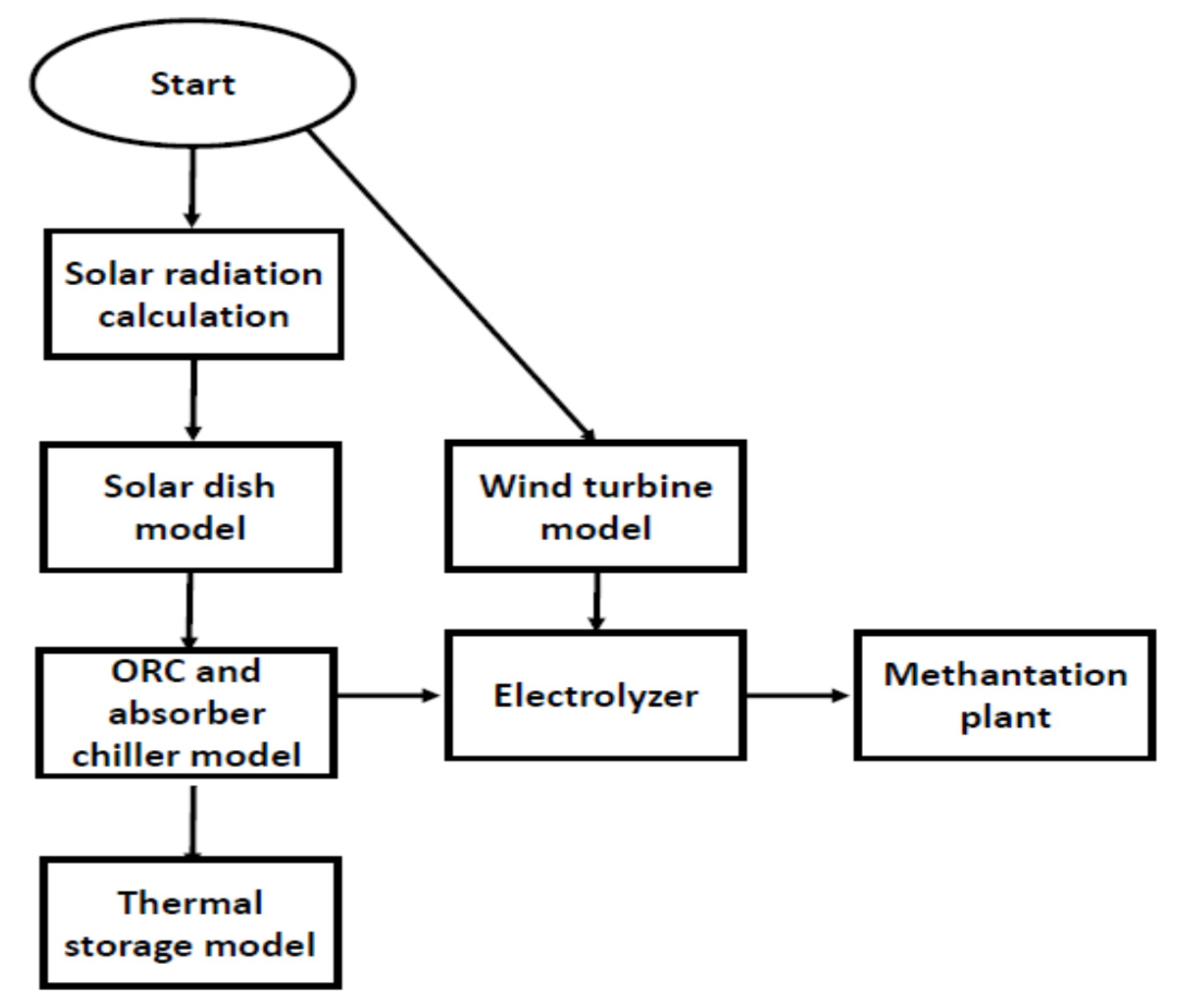
Figure 1 is a schematic diagram of the proposed system, the arrows also illustrating the process. The proposed system comprises six subsystems: solar dish, ORC, single-effect absorption chiller, proton-exchange membrane (PEM) electrolyzer, wind turbine, and methanation plant. The working fluids in the solar dish, ORC, and absorption chiller subsystems are Terminol VP-1, R134a, and lithium bromide solution, respectively. Terminol VP-1 is capable of operating under pressures of 15 bar and temperatures up to 400 [33]. R134a exhibits the highest energy and exergy efficiencies for the ORC system [33,34,35]. Water, as a refrigerant and lithium bromide as an absorbent, is one of the most used working fluid pairs in the absorption chillers [36].
Terminol VP-1 passes through a solar dish collector to absorb the solar radiation heat (1). A thermal energy storage tank is used to attenuate the fluctuations of solar radiation and for the system’s operating even during the night and to the operating fluid reach the desired temperature. The thermostat I avoids sending the Terminol at temperatures lower than 80 to the ORC’s evaporator. When the Terminol temperature is under 80 , it can be pumped through the bypass line back to the storage tank, and when it is over 80 it is pumped to the evaporator (2) of the ORC subsystem to heat the ORC working fluid. The superheated R134a enters the turbine (9) to generate power, then it passes through the condenser and it is pumped back to the evaporator to close the ORC. The electricity produced from the ORC subsystem provides part of the electricity needs in the methanation subsystem; the remaining electricity can be used to supply the electric loads or even sent to the electric grid. Thermostat II avoids sending the Terminol at temperatures lower than 60 to the absorption chiller’s generator. When the Terminol temperature is under 60 , it is sent back through a bypass line to the storage tank, and when its temperature is over 60 it enters the absorption chiller’s generator (3) to provide the heat required for the cooling products in the evaporator.
Wind turbines produce part of the electricity required by the electrolyzer. The hydrogen produced in the electrolyzer enters the methanation plant (19), where it reacts with supplied CO2 (A2) to produce CH4 syngas (A3) and steam (A4). In this way, the syngas (that has many useful applications) production is fully based on renewable sources. Besides that, cooling and power are produced simultaneously by absorption chiller, ORC, and wind turbines, respectively. Additionally, the heat released by the condenser of the absorption chiller and by the ORC condenser, oxygen released by the electrolyzer, and steam released by the methanation plant can be useful for any purpose.
The following main assumptions are considered in the system’s modeling and simulation:
  • The storage tank is used to attenuate some small system fluctuations, and it is assumed that along a day the HTF conditions when leaving the storage tank are the same as the HTF leaving the solar dish [37,38].
  • Ambient pressure and temperature are 1 atm and 15 [39]
  • The Weibull distribution density function is assumed for the wind speed in wind turbine power production [40]
  • The dish collector is assumed to be always directed to the sun
  • The efficiency of the ORC turbine and pumps are considered to be 85% [39,41]
  • For the heat exchanging components such as the condenser and the evaporator, energy effectiveness is assumed to be 85% [1,39]
  • The Terminol pressure loss is presumed to be 3% through the pipe [1,39]
  • Heat loss of components is assumed around 3% of the energy released by the hottest steam at these components [1,39]
The solar radiation and wind turbine modelling are presented in Appendix A.

2.2. Mass and Energy Balances

The following reaction occurs in the electrolyzer for water splitting [42]:
H 2 O   ( l )   +   electrical   energy     H 2   ( g )   +   1 2 O 2   ( g )
The performance of the electrolyzer can be obtained from the following equation [42,43,44]:
η V = 1.25 V elec
As the voltage efficiency of the PEM is assumed to be 72%, an operational voltage of 1.74 V is achieved. The mass flow rate of the produced hydrogen can be expressed as [42,43,44]:
m ˙ H 2 = W ˙ elec V elec F
where F represents the Faraday’s constant, 96,495 C/mole, and subscript elec denotes electrolyzer [42,43,44].
The reaction that happens in the methanation plant can be expressed as:
CO2 + 4H2 ↔ CH4 + 2H2O
The Coefficient of Performance (COP) of the absorption chiller is defined as:
COP =   Q ˙ Eva Q ˙ Gen + W ˙ P
where subscripts Eva, Gen, and p denote evaporator, generator, and chiller’s pump.
Mass and energy balances and energy efficiencies for each component of the proposed system are summarized in Table 2 [34,40,41,45,46,47].
In Table 1, T, h, c p , and m ˙ denote temperature, specific enthalpy, constant pressure specific heat, and mass flow rate, respectively. W ˙ and Q ˙ represent power and heat transfer rates. η is polythrophic efficiency. Subscripts E, T, C, and elec refer to evaporator, turbine, condenser, and electrolyzer, respectively. HHV stands for the higher heating value.
The energy efficiency of the whole system can be set as:
Energy   efficiency = W ˙ T + W ˙ windturbine , ave W ˙ p W ˙ elec +   m ˙ 21 HHV CH 4 + Q ˙ E A a G b + W ˙ windturbine , er
where subscripts E, T, P, and elec refer to the evaporator of the absorption chiller, turbine of the ORC, pumps, and electrolyzer, respectively. The energy efficiency of the whole system is the ratio between the useful energy effect of the system and the energy input required to drive it (even if it uses only renewable energy sources). The energy inputs are solar and wind energy and useful outputs are cooling at the evaporator of the absorption chiller, electricity, and produced syngas methane.

2.3. Exergy Balance

Exergy analysis is a powerful tool to identify inefficiencies of industrial processes and to improve them. Exergy comprises thermomechanical and chemical components, and it is the maximum amount of useful work that can be achieved by a system when it evolves up to reach equilibrium with the environment.
The total specific exergy of a stream is expressed as [48]:
ex = ( h h 0 ) T 0 ( s s 0 ) + T 0   x i R i   lny i +   x i ex chi + V 2 2 + gz
where h and T are enthalpy and absolute temperature, and Ri is the particular gas constant of chemical species i. xi and yi denote the mass fraction and mole fraction of chemical species i, exchi is the specific chemical exergy of chemical species i. and z, g, and v are height, gravitational acceleration, and velocity, respectively. The subscript i denotes chemical species i, and 0 refers to the environment condition (dead state).
Potential and kinetic exergy changes can be assumed negligible. Table 3 summarizes the exergy efficiency and the exergy destruction rate ( E ˙ D   ) for each component of the proposed system [49,50,51,52,53,54].
Where, for wind turbine equations, ρ represents the air density, A2 denotes the swept area of the wind turbine, and u is the wind velocity as mentioned above.
The whole system exergy efficiency can be obtained as:
Exergy   efficiency = W ˙ T W ˙ p + W ˙ windturbine , ave W ˙ elec + m ˙ 21 ex 21 Q ˙ E ( 1 T 0 T E ) A a G b   ( 1 4 3 ( T amb T sun ) + 1 3 ( T amb T sun ) 4 ) + W ˙ windturbine , er
where subscripts E, T, P, amb, 0 denote evaporator of the chiller, turbine, pumps, ambient, and dead state condition, respectively. The exergy efficiency is defined as the ratio between the useful exergy output from the system and the needed exergy input. Similar to energy efficiency, the inputs of the system are solar and wind energy and outputs are cooling at the evaporator of the absorption chiller, electricity, and produced syngas methane.

2.4. Economic Analysis

Financial analysis can provide a valuable point of view about the capital investment cost, payback period, and the system’s income cash flow. Therefore, this assessment plays a key role to bring an understanding of the financial supports and outcome of the energy system to policymakers, decision-makers, and investors. Each of the following indices is necessary to have a proper economic understanding of a system.
The total investment cost, C0, is obtained as [55,56]:
C 0 = K Solar   dish + K Absorption   chiller + K Methanation + K Elec + K ORC
where subscripts refer to the main subsystems, and K denote the investment cost of each subsystem, which are listed in Table 4, where T, P, A, and E represent the turbine, pump, surface area of the heat exchanger, and evaporator of an absorption chiller, respectively.
The yearly income cash flow of the proposed system, denoted as CF, is expressed as [55,56]:
CF = Y electrical k electrical + Y cooling k cooling + Y CH 4 k CH 4
where Y represents the yearly energy parameter, and k is the specific cost of each of the products, as detailed in Table 5.
For the investment, the Internal Rate of Return (IRR) is obtained as [55,56]:
IRR = CF C 0 [ 1 1 ( 1 + IRR ) N ]
The Net Present Value (NPV) presents the total investment gain during the lifetime of the project, which can be expressed as [55,56]:
NPV = C 0 + CF ( 1 + r ) N 1 r ( 1 + r ) N
where r and N denote discount factor and project lifetime, here considered to be 3% and 25 years, respectively. The Simple Payback Period (SPP) can be obtained as [55,56]:
SPP = C 0 CF
and the Payback Period (PP) equation is [55,56]:
PP = ln ( C F CF r . C 0 ) ln ( 1 + r )
As it can be seen, each index is independent of the others and can be taken individually. Table 3 summarizes the cost of purchase and installation of the system’s components, and Table 4 summarizes the electricity, cooling, and syngas prices.

2.5. Exergoenvironment Analysis

The exergoenvironment (exergy-environmental) study is a complement to the analysis of an energy system. This analysis clarifies the relationship between exergy destruction and environmental impact and highlights the effect of the system on the environment as caused by the system’s inefficiencies. The smaller the impact factor is, the smaller is its environmental impact, which is achievable by reducing the system’s exergy destruction rate.
The exergoenvironment factor is obtained as [64,65,66]:
f ei = Ė x tot , des   Ė x in
where Ė x tot , des and   Ė x in denote, respectively, the overall exergy destruction rate and input of exergy into the system. For an energy system, the effectiveness factor of environmental damage can be evaluated as [64,65,66]:
θ ei = f ei . C ei
where C ei represents the coefficient of exergoenvironmental impact expressed as [64,65,66]:
C ei = 1 η ex
For any energy system there is an exergoenvironmental impact improvement that illustrates the positive effect of the energy system on the environment, which can be evaluated as [64,65,66]:
θ eii = 1 θ ei
The stability factor of exergy can be obtained as [64,65,66]:
f es = Ė x tot , des Ė x tot , out + Ė x tot , des + 1

3. Result and Discussion

3.1. System Specification

In this section, the results of the modeling that was performed in the MATLAB software are reported and discussed. One main code has been written in MATLAB. Four subroutines are written for water lithium bromide properties calculation, wind turbine energy and exergy analyses, sunrise and sunset time calculation for each day of a year, and Terminol properties calculation. Refprop software was used for R134a properties calculation. The section of the program is shown in Figure 2.
The proposed system is located in the Tehran province (Iran) that has an annual average of 13 h of daylight per day. The city experiences relative humidity from 64% to 25% during a year. Moreover, the annual rainfall can range from 40.8 mm to 1.1 mm, and the wettest month of the year can have 10 rainy days [67].
Table 6 summarizes the system’s specifications, and Table 7 lists the basic parameters of the solar dish collector [51]. Table 8 includes the wind turbine specifications (model Tuge 10 kW [61]). The different thermodynamic properties for different points are from the system on 13:00 of 15th of July, which is shown in Table A2 in Appendix B.

3.2. Validation of a Model

To the best of the authors’ knowledge, no similar system has been investigated before, and it is not possible to validate the results for the whole system. However, validation can be done for all of the components of the system.
For the solar dish, Equation (A5) is used, and based on the reference [55] the mean uncertainty is less than 1%.
Ref. [71] is used for validation of the ORC results. The reported reference for the ORC has the same configuration with this paper, having a heat source temperature of 115 . The power consumption of the pump, the heat exchanging rate in the evaporator and condenser, and power production of the turbine are calculated. The physical properties of R245a are near the R134a and the conditions of both cycles are below the critical point. So, all of the main and important parameters in both cycles are checked and validated. The energy efficiency predicted by the model of the present paper is 10%, which compares well with 9.7% efficiency in [71]; the mean deviation is lower than 3%.
Ref [72] is used for validation of the absorption chiller results. In that reference are conducted the energy and exergy analyses of a lithium bromide absorption chiller with 90 generator temperature and 10 kW capacity. The COP calculated with the model is 79%, which compares well with that of 76% reported [72], the mean deviation being close to 3.7%.
The wind turbine model is validated by comparing the evaluated monthly average output of wind turbines with the power curve given on the manufacturer webpage. Figure 3 shows the results of that comparison, with a mean deviation of 3.9%.
For validation of the solar radiation, Table 1 of reference [73] is considered. In this table, the monthly average of solar radiation recorded in Iran meteorological stations from 2003 to 2010 is presented. The average error is around 3.5%, which is acceptable in engineering calculation [74].
For modeling the PEM electrolyzer, the ref [43] is used. This paper mentioned that the error of the model is 1.5% by comparing experimental results. For validation of the methanation plant, the ref [75] is considered. The deviation of methane production by Equation (4) is 2.5%. In general, by considering all of the uncertainties in various components of the system, the total error for this model is around 3.6%.

3.3. Results of Energy, Exergy Analyses

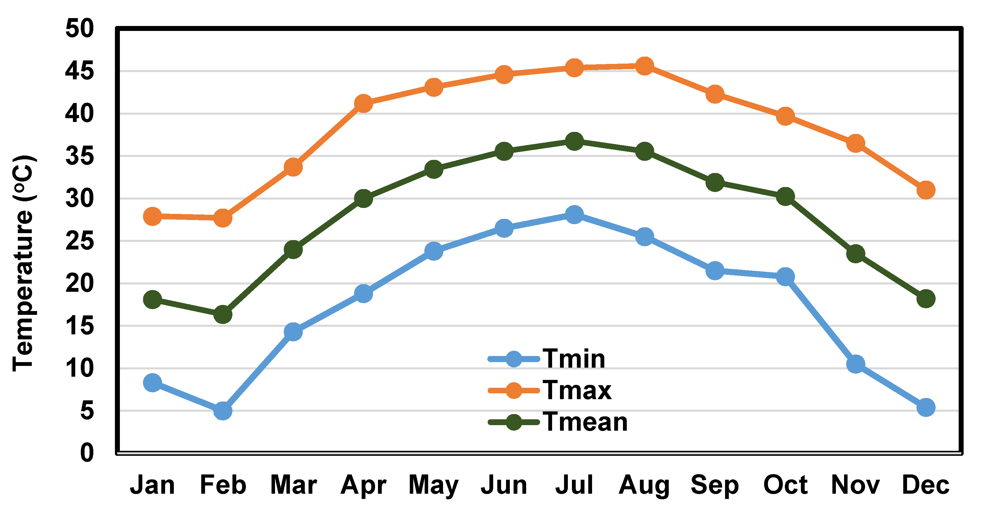
The metrological data for Tehran are presented in Appendix B. Figure 4 shows the monthly averaged useful thermal power gain of the solar dish of the proposed system for one year. As expected, this figure follows the pattern of the monthly direct solar beam in Figure A2. It is expected a system’s heat gain from solar energy changes from 1000 (in Winter) up to 2100 W (in Summer). According to Figure 4, the system may experience 52% heat gain reduction during the fall season, the maximum heat gain occurs in June and July, while the minimum heat gain occurs in December. s 1
As can be seen in Figure 5, the averaged ORC electricity production for each month of a year follows a trend similar to that of the useful heat gain from the solar dish, as the ORC energy exergy source is the solar dish heat gain. The electricity production changes from 10 W up to 170 W during a year, June and December having the maximum and minimum electricity production, respectively.
Fluctuations on the monthly averaged electricity production by the wind turbines, during a year, are presented in Figure 6. As expected, fluctuations in the wind turbine power generation follow the wind speed fluctuations presented in Figure A3. The maximum and minimum electricity power production from wind occur in May and September, respectively. The electricity production by the wind turbines ranges from 600 W up to 2700 W, which is considerably higher than the ORC power production.
Figure 7 presents the monthly averaged hydrogen production in the PEM electrolyzer for a year. As mentioned before, since electricity consumption of the PEM electrolyzer is provided mainly by wind turbines, the trend in Figure 7 is similar to the trend in Figure A3. It is observed from Figure 7 that the minimum hydrogen production, of about 170 Nm3 month−1, occurs in September. The maximum hydrogen production of about 580 Nm3 month−1 occurs in May.
Figure 8 presents the monthly averaged methane production of the methanation plant during a year. This figure follows a similar trend as that of the four previous figures, due to the direct link between the methane production in the methanation plant and the hydrogen production in the electrolyzer. The methane production rate changes from 42 Nm3 month−1 (in September) up to 140 Nm3 month−1 (in May) during a year.
Figure 9 presents the energy efficiency of ORC, the efficiency of the integration of ORC and absorption chiller, and the energy efficiency of the whole proposed system. As can be seen, the energy efficiency of the ORC system, ranging from 0.8% (in February) up to 3. 9% (in June), is smaller when compared with the other two energy efficiencies. The addition of the absorption chiller unit to the system leads to an increase in its energy performance, adding cooling production to the system using energy recovery from the thermal storage tank. After this integration, the efficiency range of the ORC + absorption chiller combination upgrades from 4.6% (in November and December) up to 12.2% (in February). It must be mentioned that in months with lower ORC energy efficiency, integration of the ORC with absorption chiller can have four or five times increase on the efficiency of the ORC + absorption chiller combination. However, in months with the higher ORC energy efficiency, the integration brings two or three times an increase in the efficiency of the ORC + absorption chiller combination. The third trend in Figure 9 refers to the energy efficiency of the whole system. As it can be observed, the energy efficiency of the whole system tends to follow a similar trend to that of the wind speed fluctuations, evidencing the major role of the wind turbines on the energy efficiency of the whole system and only a minor role of the solar radiation. The energy efficiency of the whole system changes from 9.1% (in September) up to 24.7% (in May).
Figure 10 presents the exergy efficiency of ORC, the exergy efficiency of the ORC + absorption chiller combination, and the exergy efficiency of the whole proposed system. It is seen that adding absorption chiller and wind turbines increases the exergy efficiency, even with some differences. The exergy efficiency of the ORC changes from 0.8% (in February) to 4.2% (in June). A combination of ORC with an absorption chiller increases the exergy efficiency four times in February, and the slightest increase happens in June. It is to be noted that this ORC + absorption chiller combination leads to an exergy efficiency increase that is not so notorious as the increase in energy efficiency (Figure 9). On the other hand, the exergy efficiency of the whole system is significantly enhanced because of the dominance of the products of the whole system, over the inputs when wind turbine, PEM electrolyzer, and the methanation plant are added. The exergy efficiency of the whole system changes from 8% (in September) up to 23% (in May). Similar to what happens with the previous figures, the exergy efficiency behavior tends to follow the wind speed trend, also in this case evidencing the strong dependence of the system on the wind energy and exergy.

3.4. Results of Exergoenvironment Analysis

Table 9 shows the exergoenvironment impact factor (fei), effectiveness factor of environmental damage (θei), and the stability factor of the exergy (fes).
This shows ORC, ORC + absorption chiller combination, and the whole proposed system. According to Equation (15), the exergoenvironment impact factor is directly affected by exergy destruction rate and has an inverse relation with input exergy to the system, which implies the fact that the lower this factor, the more acceptable the system. As it can be seen, adding absorption chiller and wind turbine both harm this exergoenvironment impact factor. The factor is less than 0.1 for ORC, which makes it the best system over the other two; integration of ORC and absorption chiller increases this factor to 0.2, which for the whole system this factor reaches the value of 0.7. Therefore, from the exergoenvironment impact factor, this integration is not desirable.
Similar to the exergoenvironment impact factor, the less effective factor of environmental damage, the more favorable the system. According to Equation (16), the difference in the effectiveness factor of environmental damage is that this factor is a function of exergy efficiency too, which has an inverse relation with it. This inverse relation can justify the positive impact of adding a wind turbine to the system due to its significant positive impact on the exergy efficiency of the system. Therefore, the ORC remains the best system over two, with a value of 2 of the effectiveness factor of environmental damage, and the next one is the whole system, which has a value of about 4 for this factor, and the worst case is the integration of ORC and absorption chiller with 6 for this factor.
Similarly, to the effectiveness factors of environmental damage, the case with a lower stability factor of exergy would be favorable. According to Equation (19), this factor is a function of exergy product and exergy destruction of a system. As it can be seen in Table 9, this factor is about 0.75 for ORC and the whole system, while it is about 0.9 for the unfavorable ORC + absorption chiller combination. Therefore, the proposed system has a desirable stability factor of the exergy.

3.5. Results of Economic Analysis

The results of the economic analysis are listed in Table 10. As can be seen, the SPP and PP indices for the proposed system are 15.75 and 21.6 years, respectively. Total investment cost of the system and yearly income cash flow denoted respectively as C0 and CF, are 69,665.4 and 4423.18 US$. The total investment gains during the lifetime of the project, presented as NPV, is calculated as being 5716.1 US$, and the IRR of the proposed system is 4%.

4. Conclusions

This article presents a hybrid system based on solar and wind energy for residential applications. The system can produce electricity, heating, cooling, and syngas from captured CO2. Energy, exergy, economic, and exergoenvironmental analyses (4E) are performed for the system to evaluate the performance from different viewpoints and the feasibility of the system. This proposed system can be used in regions with windy and high solar radiation condition to recover the renewable energy resources to produce electricity, syngas, heating, and cooling respectively.
The result of the system assessment can be summarized as follows:
  • The maximum and minimum electricity production from the ORC system is 170 and 10 W in Jun and December, respectively.
  • Electricity production from wind turbines ranges from 600 W in September up to 2700 in May.
  • In the methanation plant, syngas production is maximum in May about 140 Nm3 month−1, which in September experiences its lowest amount about 42 Nm3 month−1. The energy efficiency of the system changes from 24.7% (in May) to 9.1% (in September) during a year. Furthermore, annually, the exergy efficiency of the whole system ranges from 8% (in September) up to 23% (in May).
  • For those three cases, stability factors of exergy are calculated and compared. This factor for ORC, ORC + absorption chiller combination and the whole system are respectively 0.75, 0.9, 0.75. Therefore, ORC and the whole system are the best cases, and ORC + absorption chiller integration is not favorable.
  • The simple payback period and the payback period of the system are respectively 15.6 and 21.4 years. The total investment cost of the system and yearly income cash flow are 69,129.54 and 4423.18 US$. The net present value is 5818.13 US$, and the internal rate of return is 4%.

Author Contributions

S.E.; Conceptualization and Methodology. S.B.; Software and Visualization. M.A.; Conceptualization and Project administration, M.A.E.; Conceptualization, Methodology, Software, Visualization, and Writing—Original Draft. A.A.; Methodology, Software, Visualization, and Writing—Original Draft, A.A.R.; Project administration and Writing—review and Editing, B.D.; Writing—review and editing, V.A.F.C.; Writing—review and editing. A.D.; Software, Writing—review and editing and Supervision. All authors have read and agreed to the published version of the manuscript.

Funding

This research received no external funding.

Conflicts of Interest

The authors declare no conflict of interest.

Nomenclature

Variables
AaAperture of the solar dish (m2)
CFCost function ($)
C Parameter of wind turbine
C 0 Total investment cost (US$)
C e i Coefficient of exergoenvironment impact
CFIncome cash flow (US$)
CpConstant pressure specific heat (J kg−1 K−1)
COPCoefficient of performance
ESpecific parameter obtained from Equation (2)
e x Total specific exergy (J kg−1)
e x c h i Specific chemical exergy of component I (J kg−1)
E ˙ D   Exergy destruction rate (W)
FFaraday‘s constant (96,495 C mole−1)
f e i Exergoenvironment impact factor
f e s Stability factor of exergy
GbDirect normal irradiance (W m−2)
HTFHeat transfer fluid
hSpecific Enthalpy (J kg−1)
I R R Internal Rate of Return
K Parameter of wind turbine
KInvestment cost of a component (US$)
kSpecific cost of the products (US$ unit−1)
K K Number of wind turbines
LstStandard meridian for the local time zone (degrees)
LlocLongitude of the location (degrees)
HHVHigher heating value (J kg−1)
m ˙ Mass flow rate (kg s−1)
m ˙ H2Hydrogen production mass flow rate in alkaline electrolyzer (kg s−1)
NPVNet Present Value (US$)
NProject lifetime (equal to 25 years)
PPPayback period (years)
Q ˙ Heat transfer rate (W)
RUniversal gas constant: R = 8.314 (J mole−1 K−1)
rDiscount factor (equal to 3%)
SSpecific entropy (J kg−1 K−1)
SPPSimple Payback Period (years)
TTemperature ( K )
T s Solar time (s)
T l s Local solar time (s)
uWind velocity (m s−1)
ū Average wind speed (m s−1)
u c Cut-in speed (m s−1)
u r Rated speed (m s−1)
u f Furling speed (m s−1)
VVoltage (V)
W ˙ Work transfer rate (W)
xMass fraction
YYearly energy parameter
Greek Symbols
δ Deflection angle (Degree)
σStandard deviation
θ z Zenith angle (Degree)
θ e i Effectiveness factor of environmental damage
θ e i i Exergoenvironmental impact improvement Factor
β Constant parameter
φLatitude angle (Degree)
η Efficiency
η V Efficiency of the electrolyzer
θ Z Zenith angle (Degree)
ωAngle of sunset hour (Degree)
ΓGamma function
Subscripts
0Reference state condition (1 atm, 288 K)
1, 2, …, 23Points in Figure 1
ambAmbient
aveAverage
CCooling load
chiChemical energy for component i
CH4Methane ( C H 4 )
CO2Carbone dioxide ( C o 2 )
ConCondenser
elecEletrolyzer
EvaEvaporator
GenGenerator
HHeating load
PPump
SSolar
SOFCSolid oxide fuel cell
uUseful

Abbreviations

JanJanuary
FebFebruary
MarMarch
AprApril
MayMay
JunJune
JulJuly
AugAugust
SepSeptember
OctOctober
NovNovember
DecDecember

Appendix A

Appendix A.1. Solar Radiation Collection

The sunny time can be expressed as follows [76]:
Tls = Ts + 4 (Lloc − Lst) + E
where Tls and Ts denote local and solar times, respectively, Lloc is the longitude, and local standard time meridian is denoted as Lst, and E is obtained as [76]:
E = 229.2 (0.000075 + 0.001868cos β – 0.032077sin β – 0.014615 cos 2β − 0.04089 sin 2β)
β = 360 ( n 1 ) 365 , and for January first n is equal to 1. The angle of sunset hour is evaluated as [76]:
ω = arccos (−tanφ tanδ)
where φ is the latitude angle. δ is the deflection angle, evaluated as [76]:
δ = 23.45 sin ( 360 ( 284 + n ) 365 )
The thermal efficiency of the solar dish was obtained as [55]:
η th = 0.68199 0.19456 T in T am G b 0.00056 ( T in T am ) 2 G b
where Gb is the solar direct beam irradiation, and Tin and Tam are the inlets and ambient temperatures of the solar dish. This expression was obtained using a detailed numerical model, validated with experimental studies. The regression model used for that purpose has a correlation factor R2 = 0.9997 [55].
The useful heat obtained from the dish collector is evaluated as [55]:
Q ˙ u = η th Q ˙ S
Q ˙ S = A a G b
The energy balance for the storage tank is calculated as follows:
Q ˙ u = Mc p T t + m ˙ 3 h 3 m ˙ 4 h 4 m ˙ 1 h 1 Q ˙ loss
In which, M is the mass in the storage tank. Q ˙ loss   is assumed 5% of Q ˙ u .
where Aa is the aperture surface area of the solar dish, and Gb can be obtained as [76]:
G b   =   A   cos θ Z exp   ( B cos θ Z )
where θ Z denotes zenith angle, and A and B are constants [76].

Appendix A.2. Wind Energy Harvesting

The average electric power that can be produced in wind turbines is expressed as [40]:
W ˙ wind . ave = W ˙ wind . er [ exp ( ( u c C ) ) K exp ( ( u r C ) ) K ( u r C ) K ( u c C ) K exp ( ( u f C ) ) K ]
where uc, ur, and uf denote cut-in and furling speeds, and C and K can be obtained as [77,78]:
C = ū Γ ( 1 + 1 k )
K = ( σ ū ) 1.086
In these equations, ū is the average wind speed, Γ is the Gamma function, and σ denotes the wind speed standard deviation.

Appendix B

Figure A1 presents the monthly averaged minimum, maximum, and average ambient temperatures of each month for Tehran for a year. As it can be seen on the Tmax curve, August and February have the maximum and minimum ambient temperature, respectively, with 40 ambient temperature amplitude. However, according to the Tmean curve, July has the maximum ambient temperature, and the temperature of the city during a year generally ranges from 15 up to 35 .
Figure A1. Monthly averaged ambient temperature of Tehran during a year.
Energies 13 06453 g0a1
Figure A2 presents the monthly averaged direct beam solar radiation for Tehran. April, May, Jun, July, and August have significant potential for solar radiation use (spring and summer seasons). Fall and winter seasons have solar radiation below 200 W/m2 in Tehran. The direct beam radiation presents a 100% increase in June when compared with the lowest solar radiation in December.
Figure A2. Monthly- average solar radiation of Tehran during a year.
Energies 13 06453 g0a2
Table A1 shows the number of air flows in specific wind velocity ranges during various months of a year.
Figure A3 shows the monthly averaged wind velocity in each month of a year. Five different wind speed ranges are considered, and the highest average wind velocity during a year belongs to the first range for which wind speed changes from 1 to 3 m/s. Spring months reveal the highest average wind velocity in different wind speed ranges. As it can be observed in Figure A3, winter and spring seasons have the highest average wind speed, ranging from 4 to 5.5 m/s, and the lowest average wind speed occurs in summer, though December has the lowest wind speed.
Table A1. Wind velocity value at a variety of wind speed ranges for Tehran during a year [67].
Wind   Speed   ( m   s 1 ) JanFebMarAprMayJunJulAugSepOctNovDec
1 u 1 < 3 59628279717698106119966460
4 u 1 < 6 25366561536773514337318
7 u 1 < 10 15222032272775610142
11 u 1 < 16 0227123210222
u 1 > 16 000000000000
Figure A3. Monthly- average wind speed fluctuations of Tehran during a year.
Energies 13 06453 g0a3
The different thermodynamic properties for different points from the system on 13:00 of 15th of July are shown in Table A2 in Appendix B.
Table A2. The different thermodynamic properties for different points are from the system on 13:00 of 15th of July.
No.Temperature (K)Pressure (kPa)Mass Flow Rate (kg s−1)Enthalpy (kJ kg−1)
1331.250101.3001.00000794.114
2332.750202.6001.00000799.186
3345.150196.5221.00000841.966
4343.250101.3001.00000835.305
5342.710202.6001.00000833.423
6251.100121.6000.03000385.305
7250.440117.9000.03000170.139
8252.4601013.0000.03000173.024
9330.890982.6000.03000440.513
10328.1508.1280.00970122.159
11328.1503.2360.00747124.229
12316.5001.6810.0074799.302
13316.5004.4030.0097093.164
14328.1508.1280.002272576.300
15314.7008.1280.00227174.095
16316.5004.4030.00227174.095
17316.5004.4030.002272556.300
18298.300101.3000.00016105.547
19298.300101.3000.000023931.716
20298.500101.3000.00010505.969
21353.150202.6000.00004910.288
22331.210196.5001.00000793.980
23330.750190.6001.00000792.429
24329.750184.8801.00000789.064
25329.470179.3301.00000788.124
26328.890173.9501.00000786.178
27298.500101.3000.00015271.148
28353.150202.1600.00008105.547

References

  1. Alizadeh, S.; Ghazanfari, A.; Ehyaei, M.; Ahmadi, A.; Jamali, D.; Nedaei, N.; Davarpanah, A. Investigation the integration of heliostat solar receiver to gas and combined cycles by energy, exergy, and economic point of views. Appl. Sci. 2020, 10, 5307. [Google Scholar] [CrossRef]
  2. Hu, X.; Xie, J.; Cai, W.; Wang, R.; Davarpanah, A. Thermodynamic effects of cycling carbon dioxide injectivity in shale reservoirs. J. Pet. Sci. Eng. 2020, 195, 107717. [Google Scholar] [CrossRef]
  3. Jin, Y.; Davarpanah, A. Using Photo-Fenton and Floatation Techniques for the Sustainable Management of Flow-Back Produced Water Reuse in Shale Reservoirs Exploration. Water Air Soil Pollut. 2020, 231, 441. [Google Scholar] [CrossRef]
  4. Valizadeh, K.; Farahbakhsh, S.; Bateni, A.; Zargarian, A.; Davarpanah, A.; Alizadeh, A.; Zarei, M. A parametric study to simulate the non-Newtonian turbulent flow in spiral tubes. Energy Sci. Eng. 2020, 8, 134–149. [Google Scholar] [CrossRef] [Green Version]
  5. Ehyaei, M.A.; Bahadori, M.N. Internalizing the Social Cost of Noise Pollution in the Cost Analysis of Electricity Generated by Wind Turbines. Wind Eng. 2006, 30, 521–529. [Google Scholar] [CrossRef]
  6. Zarei, M.; Davarpanah, A.; Mokhtarian, N.; Farahbod, F. Integrated feasibility experimental investigation of hydrodynamic, geometrical and, operational characterization of methanol conversion to formaldehyde. Energy Sources Part A Recovery Util. Environ. 2020, 42, 89–103. [Google Scholar] [CrossRef]
  7. Ehyaei, M.; Ahmadi, A.; Rosen, M.A.; Davarpanah, A. Thermodynamic Optimization of a Geothermal Power Plant with a Genetic Algorithm in Two Stages. Processes 2020, 8, 1277. [Google Scholar] [CrossRef]
  8. Ehyaei, M.A.; Ahmadi, A.; Assad, M.E.H.; Hachicha, A.A.; Said, Z. Energy, exergy and economic analyses for the selection of working fluid and metal oxide nanofluids in a parabolic trough collector. Sol. Energy 2019, 187, 175–184. [Google Scholar] [CrossRef]
  9. Sheikhani, H.; Barzegarian, R.; Heydari, A.; Kianifar, A.; Kasaeian, A.; Gróf, G.; Mahian, O. A review of solar absorption cooling systems combined with various auxiliary energy devices. J. Therm. Anal. Calorim. 2018, 134, 2197–2212. [Google Scholar] [CrossRef]
  10. Davarpanah, A. Feasible analysis of reusing flowback produced water in the operational performances of oil reservoirs. Environ. Sci. Pollut. Res. 2018, 25, 35387–35395. [Google Scholar] [CrossRef]
  11. Davarpanah, A.; Mirshekari, B. Experimental Investigation and Mathematical Modeling of Gas Diffusivity by Carbon Dioxide and Methane Kinetic Adsorption. Ind. Eng. Chem. Res. 2019, 58, 12392–12400. [Google Scholar] [CrossRef]
  12. Ahmadi, A.; Ehyaei, M.A.; Doustgani, A.; Assad, M.e.; Hmida, A.; Jamali, D.H.; Kumar, R.; Li, Z.X.; Razmjoo, A. Recent residential applications of low-temperature solar collector. J. Clean. Prod. 2021, 279, 123549. [Google Scholar] [CrossRef]
  13. Shaygan, M.; Ehyaei, M.A.; Ahmadi, A.; Assad, M.E.H.; Silveira, J.L. Energy, exergy, advanced exergy and economic analyses of hybrid polymer electrolyte membrane (PEM) fuel cell and photovoltaic cells to produce hydrogen and electricity. J. Clean. Prod. 2019, 234, 1082–1093. [Google Scholar] [CrossRef]
  14. Ehyaei, M.; Farshin, B. Optimization of photovoltaic thermal (PV/T) hybrid collectors by genetic algorithm in Iran’s residential areas. Adv. Energy Res. 2017, 5, 31–55. [Google Scholar] [CrossRef]
  15. Ehyaei, M.A.; Ahmadi, A.; Assad, M.E.; Rosen, M.A. Investigation of an integrated system combining an Organic Rankine Cycle and absorption chiller driven by geothermal energy: Energy, exergy, and economic analyses and optimization. J. Clean. Prod. 2020, 258, 120780. [Google Scholar] [CrossRef]
  16. Ahmadi, A.; Jamali, D.; Ehyaei, M.; Assad, M.E.H. Energy, exergy, economic and exergoenvironmental analyses of gas and air bottoming cycles for production of electricity and hydrogen with gas reformer. J. Clean. Prod. 2020, 259, 120915. [Google Scholar] [CrossRef]
  17. Davarpanah, A. Parametric study of polymer-nanoparticles-assisted injectivity performance for axisymmetric two-phase flow in EOR processes. Nanomaterials 2020, 10, 1818. [Google Scholar] [CrossRef]
  18. Talebizadehsardari, P.; Ehyaei, M.; Ahmadi, A.; Jamali, D.; Shirmohammadi, R.; Eyvazian, A.; Ghasemi, A.; Rosen, M.A. Energy, exergy, economic, exergoeconomic, and exergoenvironmental (5E) analyses of a triple cycle with carbon capture. J. CO2 Util. 2020, 41, 101258. [Google Scholar] [CrossRef]
  19. Ahmadi, A.; Assad, M.E.H.; Jamali, D.; Kumar, R.; Li, Z.; Salameh, T.; Al-Shabi, M.; Ehyaei, M. Applications of Geothermal Organic Rankine Cycle for Electricity Production. J. Clean. Prod. 2020, 274, 122950. [Google Scholar] [CrossRef]
  20. Wang, X.; Zhao, L.; Wang, J.; Zhang, W.; Zhao, X.; Wu, W. Performance evaluation of a low-temperature solar Rankine cycle system utilizing R245fa. Sol. Energy 2010, 84, 353–364. [Google Scholar] [CrossRef]
  21. Wang, M.; Wang, J.; Zhao, P.; Dai, Y. Multi-objective optimization of a combined cooling, heating and power system driven by solar energy. Energy Convers. Manag. 2015, 89, 289–297. [Google Scholar] [CrossRef]
  22. Wang, J.; Yan, Z.; Wang, M.; Song, Y.; Dai, Y. Parametric analysis and optimization of a building cooling heating power system driven by solar energy based on organic working fluid. Int. J. Energy Res. 2013, 37, 1465–1474. [Google Scholar] [CrossRef]
  23. Calise, F.; d’Accadia, M.D.; Macaluso, A.; Piacentino, A.; Vanoli, L. Exergetic and exergoeconomic analysis of a novel hybrid solar–geothermal polygeneration system producing energy and water. Energy Convers. Manag. 2016, 115, 200–220. [Google Scholar] [CrossRef]
  24. Bellos, E.; Tzivanidis, C. Multi-objective optimization of a solar driven trigeneration system. Energy 2018, 149, 47–62. [Google Scholar] [CrossRef]
  25. Gogoi, T.; Saikia, S. Performance analysis of a solar heat driven Organic Rankine Cycle and Absorption Cooling System. Therm. Sci. Eng. Prog. 2019, 13, 100372. [Google Scholar] [CrossRef]
  26. El-Emam, R.S.; Dincer, I. Assessment and Evolutionary Based Multi-Objective Optimization of a Novel Renewable-Based Polygeneration Energy System. J. Energy Resour. Technol. 2017, 139, 012003. [Google Scholar] [CrossRef]
  27. Khalid, F.; Dincer, I.; Rosen, M.A. Thermoeconomic analysis of a solar-biomass integrated multigeneration system for a community. Appl. Therm. Eng. 2017, 120, 645–653. [Google Scholar] [CrossRef]
  28. El-Emam, R.S.; Dincer, I. Development and assessment of a novel solar heliostat-based multigeneration system. Int. J. Hydrog. Energy 2018, 43, 2610–2620. [Google Scholar] [CrossRef]
  29. Behzadi, A.; Habibollahzade, A.; Ahmadi, P.; Gholamian, E.; Houshfar, E. Multi-objective design optimization of a solar based system for electricity, cooling, and hydrogen production. Energy 2019, 169, 696–709. [Google Scholar] [CrossRef]
  30. Moaleman, A.; Kasaeian, A.; Aramesh, M.; Mahian, O.; Sahota, L.; Tiwari, G.N. Simulation of the performance of a solar concentrating photovoltaic-thermal collector, applied in a combined cooling heating and power generation system. Energy Convers. Manag. 2018, 160, 191–208. [Google Scholar] [CrossRef]
  31. Cavalcanti, E.J.C. Exergoeconomic and exergoenvironmental analyses of an integrated solar combined cycle system. Renew. Sustain. Energy Rev. 2017, 67, 507–519. [Google Scholar] [CrossRef]
  32. Ishaq, H.; Dincer, I.; Naterer, G. Development and assessment of a solar, wind and hydrogen hybrid trigeneration system. Int. J. Hydrog. Energy 2018, 43, 23148–23160. [Google Scholar] [CrossRef]
  33. Yousefizadeh Dibazar, S.; Salehi, G.; Davarpanah, A. Comparison of Exergy and Advanced Exergy Analysis in Three Different Organic Rankine Cycles. Processes 2020, 8, 586. [Google Scholar] [CrossRef]
  34. Darvish, K.; Ehyaei, M.; Atabi, F.; Rosen, M. Selection of optimum working fluid for organic Rankine cycles by exergy and exergy-economic analyses. Sustainability 2015, 7, 15362–15383. [Google Scholar] [CrossRef] [Green Version]
  35. Kajurek, J.; Rusowicz, A.; Grzebielec, A.; Bujalski, W.; Futyma, K.; Rudowicz, Z. Selection of refrigerants for a modified organic Rankine cycle. Energy 2019, 168, 1–8. [Google Scholar] [CrossRef]
  36. Zinet, M.; Rulliere, R.; Haberschill, P. A numerical model for the dynamic simulation of a recirculation single-effect absorption chiller. Energy Convers. Manag. 2012, 62, 51–63. [Google Scholar] [CrossRef] [Green Version]
  37. Bellos, E.; Tzivanidis, C. Parametric analysis and optimization of a solar driven trigeneration system based on ORC and absorption heat pump. J. Clean. Prod. 2017, 161, 493–509. [Google Scholar] [CrossRef]
  38. Yang, J.; Li, J.; Yang, Z.; Duan, Y. Thermodynamic analysis and optimization of a solar organic Rankine cycle operating with stable output. Energy Convers. Manag. 2019, 187, 459–471. [Google Scholar] [CrossRef]
  39. Li, Z.X.; Ehyaei, M.A.; Kasmaei, H.K.; Ahmadi, A.; Costa, V. Thermodynamic modeling of a novel solar powered quad generation system to meet electrical and thermal loads of residential building and syngas production. Energy Convers. Manag. 2019, 199, 111982. [Google Scholar] [CrossRef]
  40. Powell, W.R. An analytical expression for the average output power of a wind machine. Sol. Energy 1981, 26, 77–80. [Google Scholar] [CrossRef]
  41. Akbari, R.; Ehyaei, M.A.; Shavvon, R.S. Optimization of Solar Rankine Cycle by Exergy Analysis and Genetic Algorithm. Int.J. Energy Power Eng. 2019, 13, 630–637. [Google Scholar]
  42. Ghasemian, E.; Ehyaei, M. Evaluation and optimization of organic Rankine cycle (ORC) with algorithms NSGA-II, MOPSO, and MOEA for eight coolant fluids. Int. J. Energy Environ. Eng. 2018, 9, 39–57. [Google Scholar] [CrossRef] [Green Version]
  43. Shirmohammadi, R.; Aslani, A.; Ghasempour, R.; Romeo, L.M. CO2 utilization via integration of an industrial post-combustion capture process with a urea plant: Process modelling and sensitivity analysis. Processes 2020, 8, 1144. [Google Scholar] [CrossRef]
  44. Li, C.H.; Zhu, X.J.; Cao, G.Y.; Sui, S.; Hu, M.R. Dynamic modeling and sizing optimization of stand-alone photovoltaic power systems usinghybrid energy storage technology. Renew. Energy 2009, 34, 815–826. [Google Scholar] [CrossRef]
  45. Valizadeh, K.; Davarpanah, A. Design and construction of a micro-photo bioreactor in order to dairy wastewater treatment by micro-algae: Parametric study. Energy Sources Part A Recovery Util. Environ. Eff. 2020, 42, 611–624. [Google Scholar] [CrossRef]
  46. Asgari, E.; Ehyaei, M.A. Exergy analysis and optimisation of a wind turbine using genetic and searching algorithms. Int. J. Exergy 2015, 16, 293–314. [Google Scholar] [CrossRef]
  47. Ehyaei, M.A.; Ahmadi, A.; Rosen, M.A. Energy, exergy, economic and advanced and extended exergy analyses of a wind turbine. Energy Convers. Manag. 2019, 183, 369–381. [Google Scholar] [CrossRef]
  48. Saidi, M.; Abbassi, A.; Ehyaei, M. Exergetic optimization of a PEM fuel cell for domestic hot water heater. J. Fuel Cell Sci. Technol. 2005, 2, 284–289. [Google Scholar] [CrossRef]
  49. Bejan, A. Advanced Engineering Thermodynamics; John Wiley & Sons: Hoboken, NJ, USA, 2016. [Google Scholar]
  50. Dincer, I.; Rosen, M.A. Exergy: Energy, Environment and Sustainable Development; Newnes: New York, NY, USA, 2012. [Google Scholar]
  51. Dinçer, İ.; Midilli, A.; Kucuk, H. Progress in Exergy, Energy, and the Environment; Springer: Berlin/Heidelberg, Germany, 2014. [Google Scholar]
  52. Yousefi, M.; Ehyaei, M.; Rosen, M.A. Optimizing a New Configuration of a Proton Exchange Membrane Fuel Cell Cycle with Burner and Reformer Through a Particle Swarm Optimization Algorithm for Residential Applications. J. Electrochem. Energy Convers. Storage 2019, 16, 040801. [Google Scholar] [CrossRef]
  53. Zeinodini, M.; Aliehyaei, M. Energy, exergy, and economic analysis of a new triple-cycle power generation configuration and selection of the optimal working fluid. Mech. Ind. 2019, 20, 501. [Google Scholar] [CrossRef] [Green Version]
  54. Shirmohammadi, R.; Gilani, N. Effectiveness enhancement and performance evaluation of indirect-direct evaporative cooling system for a wide variety of climates. Environ. Prog. Sustain. Energy 2019, 38, e13032. [Google Scholar] [CrossRef]
  55. Bellos, E.; Pavlovic, S.; Stefanovic, V.; Tzivanidis, C.; Nakomcic-Smaradgakis, B.B. Parametric analysis and yearly performance of a trigeneration system driven by solar-dish collectors. Int. J. Energy Res. 2019, 43, 1534–1546. [Google Scholar] [CrossRef]
  56. Tzivanidis, C.; Bellos, E.; Antonopoulos, K.A. Energetic and financial investigation of a stand-alone solar-thermal Organic Rankine Cycle power plant. Energy Convers. Manag. 2016, 126, 421–433. [Google Scholar] [CrossRef]
  57. Alshammari, F.; Karvountzis-Kontakiotis, A.; Pesyridis, A.; Usman, M. Expander Technologies for Automotive Engine Organic Rankine Cycle Applications. Energies 2018, 11, 1905. [Google Scholar] [CrossRef] [Green Version]
  58. Lecompte, S.; Huisseune, H.; van den Broek, M.; de Schampheleire, S.; de Paepe, M. Part load based thermo-economic optimization of the Organic Rankine Cycle (ORC) applied to a combined heat and power (CHP) system. Appl. Energy 2013, 111, 871–881. [Google Scholar] [CrossRef]
  59. Quoilin, S.; Declaye, S.; Tchanche, B.F.; Lemort, V. Thermo-economic optimization of waste heat recovery Organic Rankine Cycles. Appl. Therm. Eng. 2011, 31, 2885–2893. [Google Scholar] [CrossRef] [Green Version]
  60. Schöpfer, M.D. Absorption Chillers: Their Feasibility in District Heating Networks and Comparison to Alternative Technologies. Master’s Thesis, Master of Science Degree in Energy Engineering and Management. Technical University of Lisbon, Lisbon, Portugal, 2015; p. 98. [Google Scholar]
  61. Wulf, C.; Linßen, J.; Zapp, P. Review of power-to-gas projects in Europe. Energy Procedia 2018, 155, 367–378. [Google Scholar] [CrossRef]
  62. Baier, J.; Schneider, G.; Heel, A. A Cost Estimation for CO2 Reduction and Reuse by Methanation from Cement Industry Sources in Switzerland. Front. Energy Res. 2018, 6, 5. [Google Scholar] [CrossRef] [Green Version]
  63. Bellos, E.; Tzivanidis, C.; Symeou, C.; Antonopoulos, K.A. Energetic, exergetic and financial evaluation of a solar driven absorption chiller–A dynamic approach. Energy Convers. Manag. 2017, 137, 34–48. [Google Scholar] [CrossRef]
  64. Ratlamwala, T.A.; Dincer, I.; Gadalla, M.A. Comparative environmental impact and sustainability assessments of hydrogen and cooling production systems. In Causes, Impacts and Solutions to Global Warming; Springer: Berlin/Heidelberg, Germany, 2013; pp. 389–408. [Google Scholar]
  65. Ratlamwala, T.A.; Dincer, I.; Reddy, B.V. Exergetic and Environmental Impact Assessment of an Integrated System for Utilization of Excess Power from Thermal Power Plant. In Causes, Impacts and Solutions to Global Warming; Springer: Berlin/Heidelberg, Germany, 2013; pp. 803–824. [Google Scholar]
  66. Midilli, A.; Dincer, I. Development of some exergetic parameters for PEM fuel cells for measuring environmental impact and sustainability. Int. J. Hydrog. Energy 2009, 34, 3858–3872. [Google Scholar] [CrossRef]
  67. Nakomčić-smaragdakis, B.B.; Dragutinović, N.G. Hybrid renewable energy system application for electricity and heat supply of a residential building. Therm. Sci. 2016, 20, 695–706. [Google Scholar] [CrossRef] [Green Version]
  68. Pavlović, S.R.; Bellos, E.A.; Stefanović, V.P.; Tzivanidis, C.; Stamenković, Z.M. Design, simulation, and optimization of a solar dish collector with spiral-coil thermal absorber. Therm. Sci. 2016, 20, 1387–1397. [Google Scholar] [CrossRef]
  69. Pavlovic, S.; Daabo, A.M.; Bellos, E.; Stefanovic, V.; Mahmoud, S.; Al-Dadah, R.K. Experimental and numerical investigation on the optical and thermal performance of solar parabolic dish and corrugated spiral cavity receiver. J. Clean. Prod. 2017, 150, 75–92. [Google Scholar] [CrossRef] [Green Version]
  70. Pavlovic, S.; Bellos, E.; le Roux, W.G.; Stefanovic, V.; Tzivanidis, C. Experimental investigation and parametric analysis of a solar thermal dish collector with spiral absorber. Appl. Therm. Eng. 2017, 121, 126–135. [Google Scholar] [CrossRef] [Green Version]
  71. Al-Mousawi, F.N.; Al-Dadah, R.; Mahmoud, S. Integrated adsorption-ORC system: Comparative study of four scenarios to generate cooling and power simultaneously. Appl. Therm. Eng. 2017, 114, 1038–1052. [Google Scholar] [CrossRef]
  72. Al-Tahaineh, M.F.H.; Al-Rashdan, M. Exergy Analysis of a Single-Effect Water-Lithium Bromide Absorption Chiller Powered by Waste Energy Source for Different Cooling Capacities. Energy Power 2013, 3, 106–118. [Google Scholar]
  73. Gorjian, T.T.H.S.; Ghobadian, B. Estimation of mean monthly and hourly global solar radiation on surfaces tracking the sun. In Proceedings of the 2012 Second Iranian Conference on Renewable Energy and Distributed Generation, Tehran, Iran, 6−8 March 2012; pp. 172–177. [Google Scholar]
  74. Oberkampf, W.L.; DeLand, S.M.; Rutherford, B.M.; Diegert, K.V.; Alvin, K.F. Error and uncertainty in modeling and simulation. Reliab. Eng. Syst. Saf. 2002, 75, 333–357. [Google Scholar] [CrossRef]
  75. Chwoła, T.; Spietz, T.; Więcław-Solny, L.; Tatarczuk, A.; Krótki, A.; Dobras, S.; Wilk, A.; Tchórz, J.; Stec, M.; Zdeb, J. Pilot plant initial results for the methanation process using CO2 from amine scrubbing at the Łaziska power plant in Poland. Fuel 2020, 263, 116804. [Google Scholar] [CrossRef]
  76. Duffie, J.A.; Beckman, W.A. Solar Engineering of Thermal Processes; John Wiley & Sons: Hoboken, NJ, USA, 2013. [Google Scholar]
  77. Johnson, G.L. Wind Energy Systems; Citeseer: Gaithersburg, MD, USA, 2006. [Google Scholar]
  78. Justus, C.G. Winds and Wind System Performance, Research Supported by the National Science Foundation and Energy Research and Development Administration; Franklin Institute Press: Philadelphia, PA, USA, 1978; p. 120. [Google Scholar]
Figure 1. The schematic diagram of the system.
Energies 13 06453 g001
Figure 2. The subsection and methodology of the program.
Energies 13 06453 g002
Figure 3. Results for validation of the wind turbine model.
Energies 13 06453 g003
Figure 4. Monthly averaged useful heat gain from a solar dish during a year (Location: Tehran).
Energies 13 06453 g004
Figure 5. Monthly averaged Organic Rankine Cycle (ORC) electricity production during a year.
Energies 13 06453 g005
Figure 6. Monthly averaged wind turbine electricity production during a year.
Energies 13 06453 g006
Figure 7. Monthly-average electrolyzer hydrogen production during a year.
Energies 13 06453 g007
Figure 8. Monthly-average methane production of methanation plant during a year.
Energies 13 06453 g008
Figure 9. Monthly averaged energy efficiency of the system during a year.
Energies 13 06453 g009
Figure 10. Monthly averaged exergy efficiency of the system during a year.
Energies 13 06453 g010
Table 1. The summary of key point of each research.
No.AuthorsRefSystemKey Points
1Wang et al.[20]R245a ORC solar poweredThe electrical power production is equal 1.73 kW with 45.2% isentropic efficiency
2Wang et al.[21]Solar powered ORC and ejector refrigeration cycle to produce power, heating, and coolingFor the CCP and CHP modes, the optimum average output was 5.84, 8.89 kW, respectively.
3Wang et al.[22]Solar powered triple cycle to produce electrical power, heating, and coolingThe system efficiency in CHP, CCP, and power modes is equal to 19.10%, 27.24%, and 10.47%, respectively.
4Calise et al.[23]Solar powered ORC, and multieffect distillation, absorption chiller to produce electrical power, heating, cooling, and fresh waterThe exergy efficiency is between 40% and 50% during the thermal recovery operation and it is between 16% and 20% during the cooling operation.
5Bellos and Tzivanidis[24]The ORC based hybrid system with an ejector deviceThe optimum system energy and exergy efficiencies are equal to 87% and 12%
6Gogoi and Saikia[25]Solar powered ORC with absorption chillerMaximum power is produced (1.74 MW) by the R245fa and the minimum value (1.62 MW) with Neo-pentane
7El-Emam and Dincer[26]The helium cycle and SOFC powered by solar and biomass energyThe system energy and exergy efficiencies are 39.9% and 27.5%
8Khalid et al.[27]ORC, gas cycle, and absorption chillerThe system energy and exergy efficiencies are 91.0% and 34.9%, respectively. The levelized cost of electricity is $0.117/kW h.
9El-Emam and Dincer[28]Heliostat solar receiver and steam cycleThis system produces 4 MW electric power, 1.25 kg/h of hydrogen, and 90 kg/s of fresh water
10Behzadi et al.[29]Photovoltaic/thermal cells and thermoelectric generatorThe exergy efficiency and total cost rate reach 12.01% and 0.1762$/h
11Moaleman et al.[30]Concentrating photovoltaic-thermal unit and water-ammonia absorption chillerThe system trigeneration energy efficiency reaches 58.01%
Table 2. Mass and energy balance equations and energy efficiency of the system’s components.
ComponentMass Balance EquationEnergy Balance Equation
Solar dish
Dish collector m ˙ 2 = m 3   ˙ m ˙ 2 c p ( T 3 T 2 ) = η th Q ˙ S
Pump m ˙ 1 = m ˙ 2 W ˙ p = m ˙ 1 ( h 2 s h 1 ) η p
Absorption chiller
Pump m ˙ 13 = m ˙ 10 W ˙ p = m ˙ 13 ( h 10 s h 13 ) η P
Expansion valve 1 m ˙ 15 = m ˙ 16   h 15 = h 16
Absorber m ˙ 12 + m ˙ 17 = m ˙ 13 m ˙ 17 h 17 + m ˙ 12 h 12 = m ˙ 13 h 13 + Q ˙ A
Generator m ˙ 11 + m ˙ 14 = m ˙ 10 m ˙ 10 h 10 + m ˙ 23 h 23 = m ˙ 11 h 11 ˙ + m ˙ 14 h 14 + m ˙ 24 h 24 + Q ˙ G
Condenser m ˙ 15 = m ˙ 14 Q ˙ C = m ˙ 14 ( h 14 h 15 )
Expansion valve 2 m ˙ 11 = m ˙ 12 h 11 = h 12
Evaporator m ˙ 16 = m ˙ 17 Q ˙ E = m ˙ 16 ( h 17 h 16 )
ORC
Pump m ˙ 8 = m ˙ 7 W ˙ p = m ˙ ORC ( h 8 s h 7 ) η p
Evaporator m ˙ 8 = m ˙ 9   and   m ˙ 5 = m ˙ 22 Q ˙ E = m ˙ ORC ( h 9 h 8 ) = m ˙ HTF ( h 5 h 22 )
Turbine m ˙ 6 = m ˙ 9 W ˙ T = m ˙ ORC ( h 9 h 6 s ) η T
Condenser m ˙ 6 = m ˙ 7 Q ˙ C = m ˙ ORC   ( h 6 h 7 )
PEM
PEM electrolyzer m ˙ 18 = m ˙ 27 + m ˙ 19 m ˙ 18 h 18 + W ˙ elec = m ˙ 27 h 27 + m ˙ 19 h 19
Wind turbines
Wind turbine- W ˙ wind , ave = W ˙ wind , er [ exp ( ( u c C ) ) K exp ( ( u r C ) ) K ( u r C ) K ( u c C ) K exp ( ( u f C ) ) K ]
Methanation plant
Methanation plant m ˙ 19 + m ˙ 20 = m ˙ 21 + m ˙ 28 m ˙ 19 h 19 + m ˙ 20 h 20 = m ˙ 21 h 21 + m ˙ 28 h 28
Table 3. Exergy efficiency and exergy destruction rate for each component of the proposed system.
ComponentExergy EfficiencyExergy Destruction Rate
Solar dish
Dish collector m ˙ 2 ( ex 3 ex 2 ) G b A   ( 1 4 3 ( T amb T sun ) + 1 3 ( T amb T sun ) 4 ) m ˙ 2 ( ex 3 ex 2 ) + G b A ( 1 4 3 ( T amb T sun ) + 1 3 ( T amb T sun ) 4 )
Pump m ˙ 1 ( ex 1 ex 2 ) W ˙ p m ˙ 1 ( ex 1 ex 2 ) + W ˙ p
Absorption chiller
Pump m ˙ 13 ( ex 10 ex 13 ) W ˙ p m ˙ 13 ( ex 13 ex 10 ) + W ˙ p
Expansion valve 1- m ˙ 15 ( ex 15 ex 16 )
Absorber m ˙ 13 ex 13 m ˙ 17 ex 17 + m ˙ 12 ex 12 m ˙ 17 ex 17 + m ˙ 12 ex 12 m ˙ 13 ex 13 Q ˙ A ( 1 T 0 T A )
Generator m ˙ 14 ex 14 m ˙ 10 ( ex 10 ex 11 ) + m ˙ 23 ( ex 23 ex 24 ) m ˙ 10 ( ex 10 ex 11 ) + m ˙ 23 ( ex 23 ex 24 ) m ˙ 14 ex 14 Q ˙ G ( 1 T 0 T G )
Condenser Q ˙ c ( 1 T 0 T c ) m ˙ 14 ex 14 m ˙ 15 ex 15 m ˙ 14 ex 14 m ˙ 15 ex 15 Q ˙ c ( 1 T 0 T c )
Expansion valve 2- m ˙ 11 ( ex 11 ex 12 )
Evaporator Q ˙ E ( 1 T 0 T E ) m ˙ 16 ( ex 16 ex 17 ) m ˙ 16 ( ex 16 ex 17 ) Q ˙ E ( 1 T 0 T E )
ORC
Pump m ˙ 7 ( ex 8 ex 7 ) W ˙ p m ˙ 7 ( ex 7 ex 8 ) + W ˙ p
Evaporator m ˙ 8 ( ex 9 ex 8 ) m ˙ 5 ( ex 5 ex 22 ) m ˙ 2 ( ex 5 ex 22 ) m ˙ 8 ( ex 9 ex 8 )
Turbine W ˙ T m ˙ 9 ( ex 9 ex 6 ) m ˙ 9 ( ex 9 ex 6 ) W ˙ T
Condenser Q ˙ Con ( 1 T 0 T Con ) m ˙ 6 ( ex 6 ex 7 ) m ˙ 6 ( ex 6 ex 7 ) Q ˙ Con ( 1 T 0 T c )
PEM
PEM electrolyzer m ˙ 19 ex 19 W ˙ elec + m ˙ 18 ex 18 m ˙ 18 ex 18 m ˙ 27 ex 27 m ˙ 19 ex 19 + W ˙ elec
Wind turbines
Wind turbine W ˙ windturbine , ave 8 27 ρ A 2 u 3 8 27 ρ A 2 u 3 W ˙ windturbine , ave
Methanation plant
Methanation plant m ˙ 21 ex 21 m ˙ 19 ex 19 + m ˙ 20 ex 20 m ˙ 19 ex 19 + m ˙ 20 ex 20 m ˙ 21 ex 21 m ˙ 28 ex 28
Table 4. Cost of purchase and installation of the system’s components.
ComponentCost Function ($)Source (s)
ORC
Turbine2237 ( W ˙ T ) 0.41 [57]
Pump1026 ( W ˙ p 300 ) 0.25 [58]
Condenser 0338.6   A [58]
Evaporator216.6 + 353.4 A[58,59]
Absorption chiller
Absorption chiller14,740.2095 ( Q ˙ E ) 0.6849 + 3.29 [60]
Wind turbine53,000[61]
Solar dish5650[55,56]
Storage tank2000[55,56]
Methanation500[62]
Electrolyzer2260[62]
Piping3% of total initial cost[55,56]
Table 5. The specific cost of each product for financial analysis [56,63].
Products of the SystemPrice ($ kWh−1)
kelectrical0.22
kcooling0.074
kCH40.093
Table 6. System specifications.
ParameterUnitsValue
m ˙ 1 kg s−13
            m storage kg1000
P8kPa1013
P9kPa1013
P6kPa106.4
P7kPa106.4
Δ T superheat 20
η electrolyzer -0.74
T5 110
x13-0.41
T13 43
T22 80
T23 80
Table 7. Basic parameters of the solar dish collector [51,68,69,70].
ParameterUnitsValue
Concentration ratio-28.26
Concentrator diameterm3.80
Paraboloid rim angle-45.6°
Paraboloid rim anglem2.26
Collector aperturem210.29
Spiral lengthm9.5
Spiral outer mean diametermm12.2
Spiral inner maximum diametermm11.7
Spiral inner mean diametermm10.5
Spiral inner minimum diametermm9.3
Absorber emittance-0.9
Absorber absorbance-0.9
Mirror reflectance-0.7
Distance between absorber and reflector basemm2100
Table 8. Wind turbine specification [61].
ParameterUnitsValue
W ˙ er , windturbine kW10
u c m s−13
urm s−111
ufm s−125
A2m282
Number of wind blades-3
Tower heightm18.2
Table 9. The fei, θei, and fes for ORC, ORC + absorption chiller combination and the whole proposed system.
feiθeifes
ORC0.0451.9780.758
ORC + Abs0.2206.1880.908
System0.6804.5040.762
Table 10. Economic evaluation results.
P a r a m e t e r UnitValue
SPPyears15.75
PPyears21.6
IRR%3.9
NPVUS$5716.1
C0US$69,665.4
CFUS$4423.2
Publisher’s Note: MDPI stays neutral with regard to jurisdictional claims in published maps and institutional affiliations.

