Article

Efficient Integration of Machine Learning into District Heating Predictive Models

Energy Institute, Faculty of Mechanical Engineering, Brno University of Technology—VUT Brno, Technická 2896/2, 61669 Brno, Czech Republic
*
Author to whom correspondence should be addressed.
Energies 2020, 13(23), 6381; https://doi.org/10.3390/en13236381
Submission received: 13 November 2020 / Revised: 26 November 2020 / Accepted: 28 November 2020 / Published: 2 December 2020

Abstract

:
Modern control strategies for district-level heating and cooling supply systems pose a difficult challenge. In order to integrate a wide range of hot and cold sources, these new systems will rely heavily on accumulation and much lower operating temperatures. This means that predictive models advising the control strategy must take into account long-lasting thermal effects but must not be computationally too expensive, because the control would not be possible in practice. This paper presents a simple but powerful systematic approach to reducing the complexity of individual components of such models. It makes it possible to combine human engineering intuition with machine learning and arrive at comprehensive and accurate models. As an example, a simple steady-state heat loss of buried pipes is extended with dynamics observed in a much more complex model. The results show that the process converges quickly toward reasonable solutions. The new auto-generated model performs 5 × 10⁴ times faster than its complex equivalent while preserving essentially the same accuracy. This approach has great potential to enhance the development of fast predictive models not just for district heating. Only open-source software was used, while OpenModelica, Python, and FEniCS were predominantly used.

Graphical Abstract

1. Introduction

District heating systems (DHS) are a standard solution for the supply of heat to buildings and technologies in urban areas. The proper operation of DHS can offer several synergistic advantages: higher efficiency of the central source compared to small decentralized sources, application of efficient large-scale cogeneration, reduction of specific emissions, better control over the amount of produced emissions, and use of waste heat from technologies located in different parts of the city. In recent decades, the main trends in district heating are lowering the temperature of distributed heating water, application of sophisticated systems of automatic control of DHS, utilizing renewable energy sources, development of cooperation of heating and cooling supply systems, and increasing storage capacity. Depending on heat production technology and the parameters of heat distribution, the so-called generations of heat supply systems have been defined [1]. Generations 1 to 3 include the current historical development of heating systems.
Proposals of the new 4th and recently recognized 5th generation of district heating and cooling supply systems are part of the overall answer for lowering carbon emissions. These proposals attempt to address the problem by focusing on the utilization of multiple sources of waste heat and renewables. Many of the considered sources can only provide low potential heat. This calls for lower operational temperatures in the whole DHS. It needs to be combined with some form of temperature boosting (i.e., using devices such as heat pumps) to satisfy demands for higher temperature potentials, such as those associated with domestic hot water production. The 5th generation of district heating and cooling supply goes as far as suggesting neutral temperature levels and potentially lowering the requirements for insulation of the pipes in the distribution network [2]. For efficient utilization of all possible sources, it is also necessary to deal with the temporal mismatch of demand and production. In principle, this can be realized with the help of hot and cold water storage, given that there is an efficient control strategy. The demands on control algorithms further increase with the requirements for predictive control of DHS. This requires testing a larger number of alternative scenarios, which places extreme demands on the speed of partial calculations.
If these proposals are to be fulfilled, there needs to be a systematic approach through which the behavior of these complicated systems can be studied, where new ideas can be tested in the context of the whole system and their implementation optimized, so their real potential can be assessed accurately and holistically.
It is quite straightforward to model the physics of the components (for example, using proprietary solvers for partial differential equations such as ANSYS, COMSOL, and STAR-CCM+), but it is not so straightforward to make them progress quickly as well (the exception here might be quasi-stationary models, but those are not considered strict dynamics by definition).
There are several relatively recent papers dealing with thermal modeling and optimization of district heating pipes. Teleszewski et al. presented a comparison of heat loss of a quadruple pre-insulated heating network, four pre-insulated single-pipe networks, and two twin-pipe networks. A simplified 2D steady-state model based on the boundary element method was used for calculations [3]. Krawczyk and Teleszewski also presented possible variants of heat loss reduction by analyzing possible changes in cross-sectional geometry [4,5]. Ocłon et al. studied steady-state heat losses of the pre-insulated pipe and twin-pipe in the heating network using an analytical 1D model and a numerical 2D steady-state model [6]. Heijde et al. presented the derivation of the steady-state heat losses and temperature changes for a double pipe network, which was implemented in Modelica software [7]. The authors used equivalent thermal resistances previously derived by Wallenten [8]. Danielewicz et al. developed a model for heat loss calculations in pre-insulated district heating network pipes using computational fluid dynamics (CFD) [9]. Sommer et al. compared efficiency, investment costs, and flexibility of advanced district heating systems, namely, the double-pipe bidirectional network and the single-pipe reservoir network, using Modelica simulations [10]. Arabkooshar et al. analyzed the performance of a triple-pipe system in district heating and compared it with a twin-pipe system employing CFD [11]. To combine these models into a single complex simulation of a grid might be very challenging. A fast dynamical model of a grid where the simulated physical behavior of each component is close to their real behavior opens up an opportunity for discovery and assessment of new control strategies. Such a model used to be referred to as a virtual system or digital twin, if it is a simulation of installation.
In order to bring these ideas closer to life, there needs to be an open exchange of tools, software, and data among researchers. The thriving discipline of machine learning is one example, where this attitude helps develop the technology significantly. The approach to district heating needs to be similarly bottom-up. It means that the components of the district heating and cooling systems must be modeled first. Further, they must be easy to combine into more complex simulations and the tools should be available to anyone who chooses to contribute. A recent review of open-source tools for energy-related modelling and optimization concluded that open-source development has received more attention but its success is still relatively limited [12].
Two programming languages seem to be most appropriate to the above. The first is Python, which is a general-purpose language, highly suitable for scientific computing. There is a vast amount of very competent libraries available. The other is Modelica, which is highly suitable for modelling multi-component and multi-physics dynamical systems. There is a library for modelling of district heating networks written in Modelica language called DisHeatLib [13], but it is not compatible with the open-source environment OpenModelica.
The presented research addresses the problem of generating efficient dynamical models (using open-source tools) as the means by which faster and more complex simulations of DHS can be constructed efficiently. Human engineering intuition can be efficiently combined with machine-learning algorithms into an efficient process of developing the models. An optimization tool capable of interfacing with OpenModelica as well as other software is presented in this contribution. It is capable of learning the parameters of nested Modelica models, so the models acquire the desired dynamical behavior. It can run on distributed hardware, which allows it to scale quite well for more-complicated models.
In this paper, the authors present a functional example of semi-automated model complexity reduction. First, the cross-sectional thermal dynamics behavior was modeled using the open-source tool FEniCS. Then, simple components representing thermal capacities and heat conductors were created in Modelica and a simple equivalent scheme was built from them. Then, the values of the parameters of the capacitors and heat conductors were learned, so the simplified model approximated the results of the complex model. These steps create an innovative solution process that is characterized by short computational time and robustness, corresponding to DHS needs.

2. Materials and Methods

This chapter describes the individual steps of the used calculation solution procedure. The solution to the problem can be divided into three main stages. At first, the data needs to be generated. This is achieved using an open-source platform for solving partial differential equations called the FEniCS project [14]. A serial topology generator was created for this purpose. It takes the geometry and its material properties (temperature-independent) as input and outputs topology containing mesh and its relevant annotations (see Figure 1). This topology is then loaded and passed into a finite element method assembler along with input data (driving temperatures of the water and air). An assembly object is produced, containing objects such as mass matrix, conductivity matrix, and boundary condition-related mathematical entities. The boundary conditions applied during this process are also shown in Figure 1. The open-source application ParaView is used for visualization of the domain and the spatial data.
This assembly is then passed to an adaptive time step solver. The adaptation is governed by the measurement of violation of the conservation of energy. The progress of the simulation is recorded in a comma-separated value file (CSV). The data recorded in this file are explained in Table 1. The CSV file is then converted into a Modelica package with highly efficient interpolation kernels wrapped around the data (constant computational complexity), so it can be used conveniently in the graphical OpenModelica environment and directly compiled into the executable model. This whole process is later referred to as data mining. If set, the simulator can also store snapshots of the whole domain after each time step.
The output data of this rather complex simulation must contain enough relevant dynamics. The driving temperatures used in the training dataset along with several explanatory snapshots are shown in Figure 2. It includes fast dynamics as well as long periods of equalization, so the heat has enough time to spread and affect the relevant areas if they are thermally distant from each other. Steady-state behavior is implicitly present.
In the second stage, a simplified model was implemented in Modelica. It consisted mainly of two components. The first is a thermal capacitor with a parameter, M, which represents its thermal mass. The governing equation is a simple ordinary differential equation (ODE):
M · d T d t = Q ˙ i n Q ˙ o u t
where M (J·K−1) is a thermal mass of the node, T (K) is a temperature of a node, t (s) is time, and Q · i n (W) and Q · o u t (W) are incoming and outgoing heat flow, respectively. The initial condition associated with this ODE is simply an initial value (unlike the complex model, the simple model cannot be initialized to a steady-state solution prior to the training process). The other component is the thermal conductor (or resistor, if preferred). It has a parameter, K, that represents its thermal conductance. The following equation describes its behavior:
Q ˙ 12 = K · ( T 1 T 2 )
where Q · 12 (W) is a heat flow through the conductor in direction 1–2, K (W·K−1) is a thermal conductance, and T1 (K) and T2 (K) are temperatures of the adjacent points 1 and 2, respectively. Along with these two components, there are also models representing the boundary conditions (for supply pipe, return pipe, and ground-level surface). These boundary models look up the corresponding data from the data package generated during the data-mining process. They also evaluate absolute errors between temperature and heat flow at the boundary interfaces. The total loss for training is the weighted sum of those errors from all instances of these boundary models accumulated over time.
Q ˙ m o d e l = K · ( T d a t a _ m e d i u m T m o d e l _ s u r f a c e )
where Q · m o d e l (W) is a boundary heat flow evaluated inside the simplified model, Tdata_medium (K) is a driving temperature of the media (one of Tws, Twr or Ta), which is the only input to the simplified model, and Tmodel_surface (K) is the average temperature also evaluated inside the simplified model.
L = w 1 · | T d a t a _ s u r f a c e T m o d e l _ s u r f a c e | + w 2 · | Q ˙ d a t a Q ˙ m o d e l |
where L (which has no meaningful units) is actual weighted loss or mismatch for a given surface, w1 and w2 are dimensionless weights, Tdata_surface (K) and Tmodel_surface (K) are temperatures of a corresponding surface, and Qdata_surface (K) and Qmodel_surface (K) are heat flow through the corresponding surface evaluated by complex and simplified model, respectively.
These models are then assembled into a simple grid (see Figure 3). The sparsity of the model is mostly resolved in this step. In a matrix form, the typical row would therefore have five non-zero entries, since the typical thermal capacitor is connected to four other thermal capacitors. A mathematical model of this kind should be enough to capture the macroscopic relations between variables that are recorded during the complex simulation.
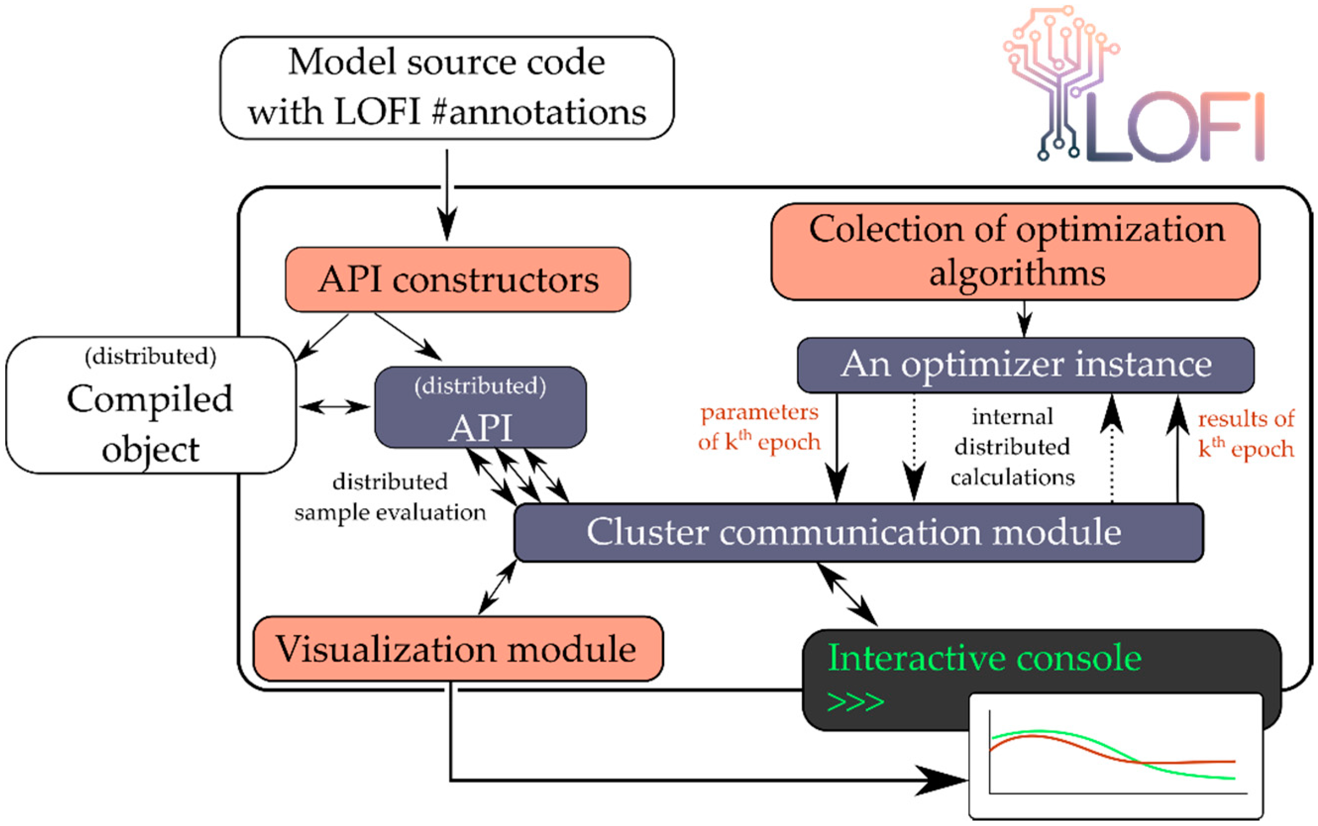
The third stage is the learning and training process. For this purpose, a custom optimization tool called Lofi was written from scratch in Python. It contains an application interface (API) to the OpenModelica compiler and several derivative-free optimizers that were also written from scratch. So far, the optimizers that were included are based on swarm intelligence and evolutionary strategies. Lofi is fully parallelized and capable of running on a distributed hardware (within a message-passing environment such as Open MPI or MPICH). Objectives and parameters subjected to optimization are annotated inside the Modelica code using the hashtags/keywords #objective and #optimize in the description of the variables (at this stage, only type Real is supported with the #optimize keyword). This overall architecture of Lofi is presented in Figure 4. The capability of Lofi is not at all limited to the problems presented in the main text of this article (see Appendix A for a short summary).

3. Results

The training and validation datasets were generated during the data-mining stage. The validation dataset was never used during the training stage. The training of the simple model was mainly performed using a particle swarm optimizer (PSO) modified by a custom adaptation strategy. This modified algorithm is referred to as a greedy random adaptation particle swarm optimizer (GRAPSO). As Lofi is still in its infancy and is missing some rather important features, such as automatic parameter scaling, the scales had to be set manually in the Modelica model. Several optimization runs have been performed to make sure that the solution is not suboptimal (convergence toward a good solution does not mean that there is no better one). Figure 5 shows the convergence of the training process performed on hardware with 40 physical CPU cores.
Next, the model was validated using the validation dataset. The results are shown in Figure 6. It shows a very good agreement with the complex model. Both the dynamical events and equilibrium state are essentially in very good agreement. The computational complexity is compared indirectly using execution times of both the complex and simple models (see Table 2). The ratio of the execution and physical time is therefore in the order of 5 × 10⁻⁹.

4. Discussion and Conclusions

Accurate dynamics of heat losses in DHS is often being excluded due to the higher computational costs associated with it. The quasi-steady solution is usually implemented instead. In the context of the 4th- and 5th-generation DHS, it might be not enough. The results presented in this paper show that machine learning provides an opportunity for substantially reducing complexity in the models of thermal dynamics. An element of the straight buried pipes forming the basic element of DHS was used as a suitable example to demonstrate the suggested optimization procedure. The example shows a very promising path toward fast and fully dynamical models with very little compromise needed. Both accuracy and speed are possible at the same time. This predestines the presented solution for use in advanced models of DHS and subsequently improves the efficiency of DHS operation. Even the modelling process is quite simple, since it is performed on a drag-and-drop basis in the graphical environment. The price that is paid is that there is no meaningful information available on temperature distribution or heat fluxes outside the three media-domain interfaces. Nevertheless, those are often the only valuable information, since they directly affect the temperature of the transported media. It is not yet clear, however, whether the complexity of the new model can be reduced even further. The future outlook is to access the performance of a model of the straight distribution line that is based on the new approach, combined with our previous contribution [15], where a fluid region is modelled. After a few minor adjustments, it should be possible to combine these models. Further, Lofi would be able to take advantage of further improvements.

Author Contributions

Conceptualization, L.K.; methodology, L.K.; software, L.K.; validation, L.K.; formal analysis, L.K.; investigation, L.K. and R.C.; resources, L.K.; data curation, L.K.; writing—original draft preparation, L.K., R.C. and J.P.; writing—review and editing, L.K., R.C. and J.P.; visualization, R.C. and L.K.; supervision, J.P.; project administration, J.P.; funding acquisition, J.P. All authors have read and agreed to the published version of the manuscript.

Funding

This paper has been supported by project Computer Simulations for Effective Low-Emission Energy Engineering” funded as project No. CZ.02.1.01/0.0/0.0/16_026/0008392 by Czech Republic Operational Programme Research, Development and Education, Priority 1: Strengthening capacity for high-quality research and the collaboration.

Conflicts of Interest

The authors declare no conflict of interest.

Appendix A

During the development of Lofi, the performance was studied in several other cases. The three most interesting examples are presented below. More details are available in the repository accessible through the https://github.com/liborkudela/lofi, the Python codes of the whole solution procedure presented in the main text of this contribution are available at https://github.com/liborkudela/pipe_physics.

Appendix A.1. Generating a Second-Order Advection Scheme for a Given Context

Lofi was used for tuning a second-order one-dimensional upwind biased advection scheme. The aim was to find a good compromise between sharp interface capturing and unwanted unphysical oscillations, which is desirable behavior in simulations of DHS. A Modelica model that is essentially a numerical simulation of advection was built. The optimization took less than a minute. The progress of the GRAPSO optimizer is shown in Figure A1. The approximation of the first-order differential operator that is being optimized has the following form:
d y i d t = u c 1 · y i 2 ( c 1 + c 2 + c 3 ) · y i 1 + c 2 · y i + c 3 · y i + 1 Δ x
where yi is the value of advected property y in node i, t is time, u is drift velocity, Δx is the distance of two adjacent nodes, and c1, c2, and c3 are the optimized coefficients. The one-dimensional domain with normalized length was discretized into 100 elements.
Figure A1. Progress of optimization in matching the value of the advected property at the outlet: ytrue is the correct analytic solution and ysol is the numerical solution.
Energies 13 06381 g0a1

Appendix A.2. Heat Transfer Inversion

In the second presented example, a heat flux at a boundary is searched for. A one-dimensional model of a thermally transient wall was coded in Modelica. The numerical solution is based on the finite difference method. One instance of this model is used to generate training data and a second one is used to simulate given input (value of second-order boundary condition distributed over time). This input is a heat flux that is meant to cause the desired temperature response on the opposite side of the wall. In this example, we used a custom optimizer named OPLES, which is a simple evolutionary strategy with isotropic Gaussian sampling, adaptive standard deviation, and parental point momentum. The optimization took about two minutes to reach the mean error of 0.001 K. The progress of the procedure is shown in Figure A2.
Figure A2. Progress in matching temperature on the opposite side of the wall, where orange is the desired temperature response and blue is the simulated response of optimized heat flux input.
Energies 13 06381 g0a2

Appendix A.3. Neural Ordinary Differential System—Lotka-Volterra System

The last example shows the ability of Lofi to learn an ODE system from data. The true system (representing the unknown ODE system) is Lotka-Volterra equations (A2). The model structure, which should learn the underlying relation from the data, is an implementation of a neural network with 50 neurons in a hidden layer, and it is formed into an ODE system (see Equation (A3)). OPLES was able to train this model within eight minutes. The progress of the training is shown in Figure A3. The advantage of neural networks lies in the fact that they can be trained into almost anything, so very little prior knowledge about the underlying mechanism hidden in the data is needed. This is also its disadvantage because the optimization process is more challenging.
x ˙ = α x β x y y ˙ = δ x y γ y
where α, β, δ, and γ are real coefficients, while x and y are the state values of the system.
[ x ˙ y ˙ ] = W 2 · t a n h ( W 1 · [ x y ] + b 1 ) + b 2
where Wi are neural weights in a matrix form, bi are neural biases in a vector form, and x, y are the state values of the system. The weights and the biases are initialized with a value of 0.1.
Figure A3. Progress of OPLES in training the neural ordinary differential equation (ODE) system: Blue and orange represent the true ODE system, while green and red represent the behavior of the optimized neural ODE system.
Energies 13 06381 g0a3

References

  1. Lund, H.; Werner, S.; Wiltshire, R.; Svendsen, S.; Thorsen, J.E.; Hvelplund, F.; Mathiesen, B.V. 4th Generation District Heating (4GDH). Integrating smart thermal grids into future sustainable energy systems. Energy 2014, 68, 1–11. [Google Scholar] [CrossRef]
  2. Revesz, A.; Jones, P.; Dunham, C.; Davies, G.; Marques, C.; Matabuena, R.; Scott, J.; Maidment, G. Developing novel 5th generation district energy networks. Energy 2020, 201, 117389. [Google Scholar] [CrossRef]
  3. Teleszewski, T.J.; Krawczyk, D.A.; Rodero, A. Reduction of Heat Losses Using Quadruple Heating Pre-Insulated Networks: A Case Study. Energies 2019, 12, 4699. [Google Scholar] [CrossRef] [Green Version]
  4. Krawczyk, D.A.; Teleszewski, T.J. Reduction of Heat Losses in a Pre-Insulated Network Located in Central Poland by Lowering the Operating Temperature of the Water and the Use of Egg-shaped Thermal Insulation: A Case Study. Energies 2019, 12, 2104. [Google Scholar] [CrossRef] [Green Version]
  5. Krawczyk, D.; Teleszewski, T. Optimization of Geometric Parameters of Thermal Insulation of Pre-Insulated Double Pipes. Energies 2019, 12, 1012. [Google Scholar] [CrossRef] [Green Version]
  6. Ocłoń, P.; Nowak-Ocłoń, M.; Vallati, A.; Quintino, A.; Corcione, M. Numerical determination of temperature distribution in heating network. Energy 2019, 183, 880–891. [Google Scholar] [CrossRef]
  7. van der Heijde, B.; Aertgeerts, A.; Helsen, L. Modelling steady-state thermal behaviour of double thermal network pipes. Int. J. Therm. Sci. 2017, 117, 316–327. [Google Scholar] [CrossRef] [Green Version]
  8. Wallentén, P. Steady-State Heat Loss from Insulated Pipes. Master’s Thesis, Byggnadsfysik LTH, Lunds Tekniska Högskola, Lund, Sweden, 1991. [Google Scholar]
  9. Danielewicz, J.; Śniechowska, B.; Sayegh, M.A.; Fidorów, N.; Jouhara, H. Three-dimensional numerical model of heat losses from district heating network pre-insulated pipes buried in the ground. Energy 2016, 108, 172–184. [Google Scholar] [CrossRef] [Green Version]
  10. Sommer, T.; Sulzer, M.; Wetter, M.; Sotnikov, A.; Mennel, S.; Stettler, C. The reservoir network: A new network topology for district heating and cooling. Energy 2020, 199, 117418. [Google Scholar] [CrossRef]
  11. Arabkoohsar, A.; Khosravi, M.; Alsagri, A.S. CFD analysis of triple-pipes for a district heating system with two simultaneous supply temperatures. Int. J. Heat Mass Transf. 2019, 141, 432–443. [Google Scholar] [CrossRef]
  12. Groissböck, M. Are open source energy system optimization tools mature enough for serious use? Renew. Sustain. Energy Rev. 2019, 102, 234–248. [Google Scholar] [CrossRef]
  13. GitHub—AIT-IES/DisHeatLib: Modelica Library for District Heating Network Modelling Using IBPSA Library as Core. Available online: https://github.com/AIT-IES/DisHeatLib (accessed on 11 November 2020).
  14. Alnaes, M.S.; Blechta, J.; Hake, J.; Johansson, A.; Kehlet, B.; Logg, A.; Richardson, C.; Ring, J.; Rognes, M.E.; Wells, G.N. The FEniCS Project Version 1.5. Arch. Numer. Softw. 2015, 3, 9–23. [Google Scholar]
  15. Kudela, L.; Chylek, R.; Pospisil, J. Performant and Simple Numerical Modeling of District Heating Pipes with Heat Accumulation. Energies 2019, 12, 633. [Google Scholar] [CrossRef] [Green Version]
Figure 1. Domain, mesh, and boundary conditions of the complex model, where q · is applied boundary heat flux, α are constant coefficients of heat transfer (αs = 600 W·K−1·m−2, αr = 600 W·K−1·m−2, αa = 20 W·K−1·m−2), T is the domain temperature, T0 is a constant temperature of the Dirichlet boundary condition, and Tws, Twr, and Ta are driving temperature of the adjacent media.
Energies 13 06381 g001
Figure 2. Driving temperatures used for training and the effect on temperature distribution inside the considered domain. The nominal values do not reflect real operational conditions, since relative values are important in inducing heat flows.
Energies 13 06381 g002
Figure 3. Model structure of the simplified physics implemented in Modelica.
Energies 13 06381 g003
Figure 4. The architecture of the Lofi optimization library.
Energies 13 06381 g004
Figure 5. The convergence of the training process (using greedy random adaptation particle swarm optimizer (GRAPSO)).
Energies 13 06381 g005
Figure 6. Accuracy of the new model for the validation dataset. Indices s, r, and a correspond to interfaces of supply, return, and air, respectively. The top part shows predicted heat flows from the domain to the adjacent media; the bottom part shows the absolute difference in predicted heat flow.
Energies 13 06381 g006
Table 1. Data recorder during the complex simulation.
NameDescriptionUnit
timesimulation times
dtthe time step used/chosen by the adaptation strategys
T_wsa driving boundary temperature of the water in the supply pipeK
T_wra driving boundary temperature of the water in the return pipeK
T_adriving boundary temperature of the airK
T_avg_sthe average temperature of the inner surface of the supply pipeK
T_avg_rthe average temperature of the inner surface of the return pipeK
T_avg_athe average temperature of the ground (top edge)K
Q_sheat flow from the domain to water to the supply pipeW/m
Q_rheat flow from the domain to water to the return pipeW/m
Q_aheat flow from the domain to the air (through top edge)W/m
Q_dbcsheat flow through locations with Dirichlet boundary conditionsW/m
Errorerror norm used for adaptationW/m
Table 2. The comparison of the computational expensiveness of both models on given datasets.
DatasetModelExecution Time on Singe CoreExecution Time Using 40 CPU CoresSingle-Core Speedup Ratio
TrainingFEniCS1915 s125 s47,875
OpenModelica0.04 snot performed
ValidationFEniCS1180 s71 s51,305
OpenModelica0.023 snot performed
Publisher’s Note: MDPI stays neutral with regard to jurisdictional claims in published maps and institutional affiliations.

