Multitask Support Vector Regression for Solar and Wind Energy Prediction

Abstract

Given the impact of renewable sources in the overall energy production, accurate predictions are becoming essential, with machine learning becoming a very important tool in this context. In many situations, the prediction problem can be divided into several tasks, more or less related between them but each with its own particularities. Multitask learning (MTL) aims to exploit this structure, training several models at the same time to improve on the results achievable either by a common model or by task-specific models. In this paper, we show how an MTL approach based on support vector regression can be applied to the prediction of photovoltaic and wind energy, problems where tasks can be defined according to different criteria. As shown experimentally with three different datasets, the MTL approach clearly outperforms the results of the common and specific models for photovoltaic energy, and are at the very least quite competitive for wind energy.

1. Introduction

There is a worldwide energy transition towards renewable sources, with a particular emphasis in wind and solar generation, which implies, among other things, a great demand by transmission system operators, wind and solar farm managers or market agents, of accurate energy forecasts to be made at the time horizons of interest for each actor. These go from the very short (up to one hour), short (up to a few hours), or medium-long (from one to several days ahead). In this work, we will deal with a particular case of the latter, namely, the hourly, day-ahead prediction, where tomorrow’s energy production at each hour must be predicted today.

Machine learning (ML) techniques have a growing presence among the different approaches to renewable energy forecasting. ML models require first to choose the predictive features to be used, which depends again on the forecasting horizon. For instance, in short-term prediction one can use past energy production values and/or real-time meteorological information, if available; on the other hand, for medium–long forecasts the features more widely used are those derived from numerical weather predictions (NWPs) provided by entities such as the European Centre for Medium-Range Weather Forecasts (ECMWF; the ones we will use) or the National Centers for Environmental Prediction (NCEP). For the day-ahead energy predictions of interest here, we will use the NWP forecasts given in today’s ECMWF run at 00 $\mathrm{UTC}$ to predict either PV or wind energy production for tomorrow’s hours between 00 and 23 $\mathrm{UTC}$. In other words, we use NWP forecasts from the 00 $\mathrm{UTC}$ run to predict energy production on the horizons between 24 and 47 h.

Once the predictive features are selected, the usual ML approach is to choose the method deemed to be better suited to the problem at hand, carefully adjust the model hyperparameters and finally build, exploit, and maintain the optimally hyperparametrized model. In particular, we can either build local models for a single installation or global models for all the installations within a more or less large geographic area. Many ML models have been proposed for renewable energy prediction, and in Section 2 we give a literature review with a particular emphasis on MTL methods.

However, any ML approach has to handle the behavior of either a single wind or solar farm or of a collection of them, behavior that may change substantially according to different time or operating conditions. This is obviously the case in photovoltaic (PV) energy, which presents markedly hourly effects and where an installation behavior at midday is very different from that at sunrise or sunset. The same can be said about seasonal effects, with summers obviously having stronger radiation and more stable atmospheric conditions than winters. Turning our attention to wind energy, the effect of individual hours in a farm’s production is much less substantial than in the PV case, but the day–night shift in the boundary layer behavior can have substantial effects on wind farms [1] and, therefore, be also reflected in the energy produced. A second example is the effect of wind direction on the output of a wind farm, as they are usually built to take advantage of the prevalent wind directions at their sites. Finally, the power curve of wind turbines has three different response zones: a first one for low speed and near zero production, an intermediate one with power growing with wind velocity and a third one, with maximum constant power up to a cut-off speed.

Of course, a way to overcome and take advantage of these dependencies is to build independent models for specific, say, hours or directions which, nevertheless, could benefit from their interactions with global models. This points to the interest of taking into account global behavior when building models targeted to specific hours or directions. Multitask learning (MTL) is a ML framework that tries precisely to do that by training all the individual models jointly with a global one, while allowing each of them to adjust to its individual task. MTL has grown enormously since its proposal by R. Caruana [2], and MTL approaches have been proposed for the main ML paradigms; recent surveys can be found in [3,4], see also Section 2. In this work, we will apply an MTL approach to support vector regression (SVR), first proposed in [5], using the convex formulation of the work in [6] for the prediction of wind and solar energy. More precisely, and besides a thorough yet still simple review of the main ideas and issues in convex MTL-SVR which may be of independent interest, our main contributions are as follows.

• The introduction of several tasks in PV and wind energy prediction in order to apply MTL approaches to both problems.
• The proposal of convex MTL-SVR for the hourly PV energy prediction under two basic multitask scenarios—hour-based tasks and season-based tasks—as well as their combination; we will show MTL models to outperform either a common or task specific models.
• The proposal of convex MTL-SVR for the hourly wind energy prediction under three basic multitask scenarios: wind angle-based tasks, wind speed-based tasks, and day–night-based tasks, as well as their combinations; here, we will show that, while not beating a common SVR model, they still offer very competitive performances.

For PV energy, we will deal with the overall production of the islands of Majorca on the Mediterranean Sea and Tenerife on the Atlantic Ocean; for wind energy, we will work with production data of the Sotavento wind farm in Northwestern Spain. The rest of the paper is organized as follows. After a literature overview in Section 2, in Section 3 we will review convex MTL-SVR from a theoretical point of view and discuss our implementation details. In Section 4, we will apply MTL-SVR to the prediction of hourly PV and wind energy production. Finally, the paper will end in Section 5 with a short discussion and conclusions section, as well as pointers to further work.

2. Literature Review

As mentioned, the ML literature for renewable energy is very large. In the case of wind energy, the works in [7,8,9] are general reviews of the application of ML models while the authors of [10,11] propose concrete models for more specific prediction horizons. For solar energy, there is again a very large body of literature addressing many different approaches to short, medium, and long term solar irradiation and energy forecasting; recent surveys include the works in [12,13,14] and a good comprehensive reference for many aspects of solar energy can be found in [15]; to these we may add the works in [16,17,18]. For its part, multitask learning (MTL) was first introduced by R. Caruana [2] and MTL approaches have been proposed for the main ML paradigms. Many advantages of MTL have been pointed out in the literature. The first one is obviously the learning of relationships between tasks that, in turn, allows their grouping through the common model, which brings together different tasks instead of letting them behave independently [19,20,21,22]. Another one is the learning of characteristics in a common representation that is sufficiently expressive for all the tasks; in particular, for neuronal models, this can be enforced through a weight matrix which reflects task relationships and can facilitate subsequent learning [23]. Recently, MTL machine learning models have started to be used for several aspects of renewable energy prediction, such as ramp events [24], wind turbine output [25], solar panel outputs [26], or ultra-short PV production [27]. Similarly, Support Vector Regression has been widely used in renewable energy prediction [10,28]. However, and to the best of our knowledge, this contribution is the first paper where multitask SVR models have been considered for the prediction of wind and solar energy production.

On the other hand, it can be safely said that MTL variants have been proposed for all the leading ML paradigms [3] and, particularly, for deep networks [4]. As shown in [29], there are multiple architectures and optimization strategies to apply MTL in a deep learning framework. However, a common trait in deep MTL is that multiple outputs, each corresponding to a different task, are produced for a given single input. The simplest such MTL model is the so-called hard parameter sharing network [28], which uses shared layers for the initial hidden layers and task-specific layers in the final ones. As said before, the overall goal is to try to find a common feature representation for all the tasks through the shared weight layers that is then exploited to derive task specific models in the network’s final layers; in particular, all tasks share the same initial features. More advanced approaches have been developed such as cross-stitch networks [28], sluice networks [28], or neural discriminative dimensionality reduction [28]; the goal of all these strategies is to share knowledge during the construction of the tasks features, from which the models are built.

In this work, however, we will consider a support vector machine (SVM) approach to MTL which, while also striving to derive better models through multitasking, presents a fundamental difference with the previously mentioned deep network-based MTL models. In fact, in the SVM-based MTL, the goal is to simultaneously train a combination of a single model common to all tasks with several task-specific models. Each one of these individual models is built upon task-specific features, which are only jointly processed by the global model and the individual task specific one. Here, the role of the common model is to somehow connect the specific models so that their behavior is harmonized across all tasks. A first reference is the work of Evgeniou and Pontil [30], where they propose an MTL-SVM approach that combines a common model, which learns from all the tasks, and task-specific models. The authors take advantage of the general theory of SVMs to write both primal and dual MTL problems, ending up with a minimization problem that can be easily solved using standard SVM procedures. This work was extended in [31], where it was shown how a variety of kernel methods can be easily adapted to an MTL framework by choosing an appropriate kernel. More specifically, they show how, in a kernelized setting, MTL problems, where the task models are related through particular regularizations, are equivalent to writing a common task problem with a proper MTL kernel. At the same time, Vapnik introduced a new general paradigm, learning using privileged information (LUPI) [32], in which group information in the data is used to try to correct the predictions made by the model. These corrections may take place in different spaces, yielding more flexible models. In particular, Vapnik proposed the SVM+ method, which embodies the LUPI approach while controlling the capacity of both the decision and correcting parts of the model. Liang showed the connection between SVM+ and MTL-SVMs in [33] and proved the efficiency of the MTL-SVMs in a biomedical application in [34].

More closely related to our approach in this paper, Cai and Cherkasski [35] also worked in the connection between SVM+ and MTL-SVMs, as well as in an MTL-SVM model including task-specific biases. Moreover, in [5] they proposed the generalized SMO (GSMO) algorithm to solve the dual problem when multiple bias are considered in the MTL-SVM. This model is very flexible and potent, as it uses common and task-specific kernels as well as individual biases; however, it requires the selection of multiple hyperparameters and efficient SVM solvers such as the LIBSVM library can no longer be applied [36]. To try to mitigate this problem, gaussian processes are proposed in [37] to select these hyperparameters.

A very important hyperparameter is the one controlling the balance between the task-specific and common models. Large values of this parameter give place to a large contribution of the common models and a small one for the specific models, while with small values of the parameter the opposite happens. However, the range of this parameter in [5] is the entire positive half real line, which makes difficult the selection of an optimal value. Moreover, it is not clear beforehand if there is any limiting relation between the MTL model and the common and independent tasks. To avoid this, we have proposed in [6] a new convex formulation of the MTL-SVM, in which this balancing parameter is replaced by a convex combination of the common and task-specific models, governed by a parameter whose domain is the range $[0,1]$. In particular, the extreme 0 and 1 values correspond to common task learning (CTL) and independent task learning (ITL), respectively. We review it next.

3. Convex Multi-Task Support Vector Regressor

Gaussian support vector machine models are widely used in regression tasks under the support vector regression (SVR) formulation. In fact, SVR models are almost always very competitive because of the approximation capabilities that Gaussian kernels lend them and the extra flexibility that the $ϵ$-insensitivity parameter in their loss provides to tailor models to specific target and noise conditions. A drawback in large sample problems is their training cost, at least quadratic in sample size; on the other hand, SVR training solves a convex problem and has thus a unique solution, in contrast with the random nature of, for instance, neural networks.

In more detail, given a sample $\{({\mathbf{x}}_i,y_i),i=1,\cdots ,N\}$ and assuming for simplicity a linear setting, a linear SVR model $f\left(\mathbf{x}\right)=\mathbf{w}·\mathbf{x}+b$ is built by solving the following primal problem,

$$\begin{array}{cccc}\hfill & \underset{\mathbf{w},b,\xi ,\widehat{\xi }}{\mathrm{arg\; min}}\hfill & \hfill & C\sum _{i=1}^N({\xi }_i+\widehat{{\xi }_i})+\frac{1}{2}{∥\mathbf{w}∥}^2\hfill \\ \hfill & \mathrm{s}.\mathrm{t}.\hfill & \hfill & \mathbf{w}·{\mathbf{x}}_i+b\ge y_i-ϵ-{\xi }_i,i=1,\cdots ,N,\hfill \\ \hfill & \hfill & & \mathbf{w}·{\mathbf{x}}_i+b\le y_i+ϵ+\widehat{{\xi }_i},i=1,\cdots ,N,\hfill \\ \hfill & \hfill & & {\xi }_i,\widehat{{\xi }_i}\ge 0,i=1,\cdots ,N,\hfill \end{array}$$

(1)

where $ϵ$ is the width of the error-insensitive tube. Note that the objective function has two components: the error minimization term, involving the ${\xi }_i$ and ${\widehat{\xi }}_i$ slacks, and the regularization term, i.e., the norm of the $\mathbf{w}$ vector. While having a simple quadratic cost function, the high number of affine constraints in (1) (two for each pattern) suggests to solve a simpler dual problem, to which one can arrive through Lagrangian theory. More concretely, the SVR dual problem is

$$\begin{array}{cccc}\hfill & \underset{\mathit{\alpha },\mathit{\beta }}{\mathrm{arg\; min}}\hfill & \hfill & \frac{1}{2}{(\mathit{\alpha }-\mathit{\beta })}^{⊺}\mathbf{Q}(\mathit{\alpha }-\mathit{\beta })+{\mathbf{y}}^{⊺}(\mathit{\alpha }-\mathit{\beta })-ϵ{\mathbf{1}}^{⊺}(\mathit{\alpha }+\mathit{\beta })\hfill \\ \hfill & \mathrm{s}.\mathrm{t}.\hfill & \hfill & 0\le {\alpha }_i,{\beta }_i\le C,i=1,\cdots ,N,\hfill \\ \hfill & \hfill & & \sum _{i=1}^N({\alpha }_i-{\beta }_i)=0,\hfill \end{array}$$

(2)

where ${\mathit{\alpha }}^{⊺}=({\alpha }_1,\cdots ,{\alpha }_N)$, ${\mathit{\beta }}^{⊺}=({\beta }_1,\cdots ,{\beta }_N)$, $\mathbf{1}$ is the vector of N ones and, in the linear case, $\mathbf{Q}$ is the dot product matrix with components ${\mathbf{Q}}_{ij}={\mathbf{x}}_i·{\mathbf{x}}_j$. To get nonlinear models, $\mathbf{Q}$ is defined in terms of a positive definite kernel, with the Gaussian one $k({\mathbf{x}}_i,{\mathbf{x}}_j)=exp(\gamma \parallel {\mathbf{x}}_i-{\mathbf{x}}_j{\parallel }^2)$ being the usual choice. Here, $\gamma$ denotes the kernel scale, a third hyperparameter after C and $ϵ$ that must be optimized; see in [38] for more details.

In an MTL setting, the global sample splits into T different subsamples $\{({\mathbf{x}}_i^r,y_i^r),i=1,\cdots ,m_r,r=1,\cdots ,T\}$ with sizes $m_r$, each of which defines an individual task. The standard SVR formulation does not use task information and in principle this would leave us with two opposed possibilities. The first, which we will call common task learning SVR (ctlSVR), fits a single SVR model over the entire dataset. The second is to fit a specific model for each task subsample; we will call this independent task learning SVR (itlSVR). However, it is possible to use task information using an MTL-SVR formulation, as proposed by Cai and Cherkasski in [35], and in [6] we have given a simpler, convex MTL-SVR formulation which we showed to be equivalent to that in [35], but with the advantage of a clear identification of the interplay between the common and independent tasks. In more detail, the primal problem of this approach, which we will call mtlSVR, is

$$\begin{array}{cccc}\hfill & \underset{\mathbf{w},{\mathbf{v}}_r,b_t,\xi ,\widehat{\xi }}{\mathrm{arg\; min}}\hfill & \hfill & \sum _{r=1}^T{C}_r\sum _{i=1}^{m_r}({\xi }_i^t+\widehat{{\xi }_i^t})+\frac{1}{2}\sum _{r=1}^T{∥{\mathbf{v}}_r∥}^2+\frac{1}{2}{∥\mathbf{w}∥}^2\hfill \\ \hfill & \mathrm{s}.\mathrm{t}.\hfill & \hfill & {\lambda }_r\left(\mathbf{w}·{\mathbf{x}}_i^r\right)+(1-{\lambda }_r)\left({\mathbf{v}}_r·{\mathbf{x}}_i^r\right)+b_r\ge y_i-{ϵ}_r-{\xi }_i^t,\hfill \\ \hfill & \hfill & & {\lambda }_r\left(\mathbf{w}·{\mathbf{x}}_i^r\right)+(1-{\lambda }_r)\left({\mathbf{v}}_r·{\mathbf{x}}_i^r\right)+b_r\le y_i+{ϵ}_r+\widehat{{\xi }_i^t},\hfill \\ \hfill & \hfill & & {\xi }_i^r,\widehat{{\xi }_i^r}\ge 0,i=1,\cdots ,m_r,r=1,\cdots ,T.\hfill \end{array}$$

(3)

Thus, the model to be learned is the convex combination $({\lambda }_r\mathbf{w}+(1-{\lambda }_r){\mathbf{v}}_r)·{\mathbf{x}}_i^r$ of the common $\mathbf{w}$ and task specific ${\mathbf{v}}_r$ components; the mixing ${\lambda }_r$ is a hyperparameter to be learned within the range $[0,1]$. Notice that with this formulation (3) reduces to the independent itlSVR models when ${\lambda }_r=0$, while for ${\lambda }_r=1$ it contains the ctlSVR model when $C_r=C$ and ${ϵ}_r=ϵ$ for all r (that is, a common C and $ϵ$ pair is used). The dual of (3) is now

$$\begin{array}{cccc}\hfill & \underset{\mathit{\alpha },\mathit{\beta }}{\mathrm{arg\; min}}\hfill & \hfill & \frac{1}{2}{(\mathit{\alpha }-\mathit{\beta })}^{⊺}\widehat{\mathbf{Q}}(\mathit{\alpha }-\mathit{\beta })+{\mathbf{y}}^{⊺}(\mathit{\alpha }-\mathit{\beta })-\sum _{r=1}^T{ϵ}_r\sum _1^{m_r}\left({\alpha }_i^r-{\beta }_i^r\right)\hfill \\ \hfill & \mathrm{s}.\mathrm{t}.\hfill & \hfill & 0\le {\alpha }_i^r,{\beta }_i^r\le C_r,i=1,\cdots ,m_r,r=1,\cdots ,T,\hfill \\ \hfill & \hfill & & \sum _{i=1}^{m_r}({\alpha }_i^r-{\beta }_i^r)=0,r=1,\cdots ,T,\hfill \end{array}$$

(4)

which is also obtained through Lagrangian theory. Here, the matrix $\widehat{\mathbf{Q}}$ has the form

$$\widehat{\mathbf{Q}}=\Lambda \mathbf{Q}\Lambda +({\mathbf{I}}_N-\Lambda )\mathbf{K}({\mathbf{I}}_N-\Lambda ),$$

with $N={\sum }_r{m}_r$, ${\mathbf{I}}_N$ the $N\times N$ identity matrix and $\Lambda$ being the following diagonal matrix

$$\underset{N\times N}{\Lambda }=\left[\begin{array}{ccc}{\Lambda }_1& & \\ & \ddots & \\ & & {\Lambda }_T\end{array}\right],$$

that is, a block diagonal matrix, where each block ${\Lambda }_r$ is in turn another diagonal matrix ${\Lambda }_r={\lambda }_r{\mathbf{I}}_{m_r}$. In the linear setting of (4), $\mathbf{Q}$ is the dot product matrix with entries ${\mathbf{x}}_i^r·{\mathbf{x}}_j^s$ and $\mathbf{K}$ is a block diagonal matrix with entries ${\delta }_{rs}({\mathbf{x}}_i^r·{\mathbf{x}}_j^s)$, $1\le r,s\le T$, where ${\delta }_{rs}$ is the Kronecker delta function. In a kernel setting, $\mathbf{Q}$ is computed using the common kernel $k({\mathbf{x}}_i^r,{\mathbf{x}}_j^s)$ that mixes patterns coming from all tasks, and $\mathbf{K}$ is again a block diagonal matrix computed now using the kernels ${\delta }_{rs}{k}_r({\mathbf{x}}_i^r,{\mathbf{x}}_j^s)$, $1\le r,s\le T$, where $k_r$ is a kernel specific to task r. More specifically, we can write the multitask kernel to compute $\widehat{\mathbf{Q}}$ as

$$\widehat{k}({\mathbf{x}}_i^r,{\mathbf{x}}_j^s)={\lambda }_r{\lambda }_{s}k({\mathbf{x}}_i^r,{\mathbf{x}}_j^s)+{(1-{\lambda }_r)}^2{\delta }_{rs}{k}_r({\mathbf{x}}_i^r,{\mathbf{x}}_j^s).$$

Notice that tasks are not mixed in $\mathbf{K}$, that is, given two patterns from tasks r and s, we have that the specific kernel ${\delta }_{rs}{k}_r({\mathbf{x}}_i^r,{\mathbf{x}}_j^s)=0$ if $r\ne s$. While quite flexible, this general approach has the drawback of the high number of hyperparameters involved, namely, a triplet $\left(C_r,{ϵ}_r,{\lambda }_r\right)$ for each multi-task model, plus common and specific kernel widths $\left(\gamma ,{\gamma }_r\right)$ if, for instance, Gaussian kernels are used, that is, $4\times T+1$ in total. To alleviate this, we will simplify the general formulation in (4) by considering first only a common selection of the $\left(C,ϵ,\lambda \right)$ hyperparameters, and using the $\gamma$ scalings of the individual common and independent kernels. Problem (4) becomes now

$$\begin{array}{cccc}\hfill & \underset{\mathbf{w},{\mathbf{v}}_r,b_t,\xi ,\widehat{\xi }}{\mathrm{arg\; min}}\hfill & \hfill & C\sum _{r=1}^T\sum _{i=1}^{m_r}({\xi }_i^t+\widehat{{\xi }_i^t})+\frac{1}{2}\sum _{r=1}^T{∥{\mathbf{v}}_r∥}^2+\frac{1}{2}{∥\mathbf{w}∥}^2\hfill \\ \hfill & \mathrm{s}.\mathrm{t}.\hfill & \hfill & \lambda \left(\mathbf{w}·{\mathbf{x}}_i^r\right)+(1-\lambda )\left({\mathbf{v}}_r·{\mathbf{x}}_i^r\right)+b_r\ge y_i-ϵ-{\xi }_i^t,\hfill \\ \hfill & \hfill & & \lambda \left(\mathbf{w}·{\mathbf{x}}_i^r\right)+(1-\lambda )\left({\mathbf{v}}_r·{\mathbf{x}}_i^r\right)+b_r\le y_i+ϵ+\widehat{{\xi }_i^t},\hfill \\ \hfill & \hfill & & {\xi }_i^r,\widehat{{\xi }_i^r}\ge 0,i=1,\cdots ,m_r,r=1,\cdots ,T.\hfill \end{array}$$

(5)

Notice that when $\lambda =1$, mtlSVR reduces to the common model ctlSVR; when $\lambda =0$, however, we get a simplified version of the itlSVR models where all of them share common $\left(C,ϵ\right)$ hyperparameters. As for standard SVMs, the problem actually solved is the dual of (5), namely,

$$\begin{array}{cccc}\hfill & \underset{\mathit{\alpha },\mathit{\beta }}{\mathrm{arg\; min}}\hfill & \hfill & \frac{1}{2}{(\mathit{\alpha }-\mathit{\beta })}^{⊺}\widehat{\mathbf{Q}}(\mathit{\alpha }-\mathit{\beta })+{\mathbf{y}}^{⊺}(\mathit{\alpha }-\mathit{\beta })-ϵ{\mathbf{1}}^{⊺}(\mathit{\alpha }+\mathit{\beta })\hfill \\ \hfill & \mathrm{s}.\mathrm{t}.\hfill & \hfill & 0\le {\alpha }_i^r,{\beta }_i^r\le C,i=1,\cdots ,m_r,r=1,\cdots ,T,\hfill \\ \hfill & \hfill & & \sum _{i=1}^{m_r}({\alpha }_i^r-{\beta }_i^r)=0,r=1,\cdots ,T,\hfill \end{array}$$

(6)

where $\mathit{\alpha },\mathit{\beta }$, and $\mathbf{1}$ are defined as in (2). However, observe now the multiple equality constraints in (6), in contrast with the single equality constraint in (2); they appear as a consequence of the multiple biases $b_r$ in (5). The dual (6) is again obtained through Lagrangian theory; see in [6] for more details, where it is also shown that the multi-task kernel matrix $\widehat{\mathbf{Q}}$ has the form

$$\widehat{\mathbf{Q}}={\lambda }^2\mathbf{Q}+{(1-\lambda )}^2\mathbf{K},$$

and we can write now the multitask kernel to compute $\widehat{\mathbf{Q}}$ as

$$\widehat{k}({\mathbf{x}}_i^r,{\mathbf{x}}_j^s)={\lambda }^{2}k({\mathbf{x}}_i^r,{\mathbf{x}}_j^s)+{(1-\lambda )}^2{\delta }_{rs}{k}_r({\mathbf{x}}_i^r,{\mathbf{x}}_j^s).$$

Finally, the multi-task prediction over a new pattern ${\mathbf{z}}^t$ from task t is

$$f_{\mathrm{mtl}}\left({\mathbf{z}}^t\right)={\lambda }^2\sum _{r=1}^T\sum _{i=1}^{m_r}\left[{\left({\alpha }_i^r\right)}^{\ast }-{\left({\beta }_i^r\right)}^{\ast }\right]k({\mathbf{x}}_i^r,{\mathbf{z}}^t)+{(1-\lambda )}^2\sum _{i=1}^{m_t}\left[{\left({\alpha }_i^t\right)}^{\ast }-{\left({\beta }_i^t\right)}^{\ast }\right]k_t({\mathbf{x}}_i^t,{\mathbf{z}}^t)+b_t^{\ast }.$$

(7)

We point out that, in order to apply the standard LIBSVM SMO solver [36] to (6), we will work with a single global bias b instead of the task specific biases $b_r$ that appear in (5) and (7).

In what follows, we will apply this last convex MTL simplification, that is, we will solve (6) with a common bias b for all tasks, as well as common hyperparameters $\left(C,ϵ,\lambda \right)$. We shall also work with common and task specific Gaussian kernels, for which we use the optimal widths $\gamma$ and ${\gamma }_r$, $1\le r\le T$, of the ctlSVR model and the itlSVR models, respectively. The advantage of using a common bias is that we can, as mentioned, directly use an SMO solver, but the price to pay is to have less flexible models. Moreover, and as mentioned, in our approach having $\lambda =1$ reduces the MTL models to the lcommon ctlSVR one; however, when $\lambda =0$, the MTL models do not coincide with the itlSVR ones, as these use their own $C_r$ and ${ϵ}_r$ hyperparameters, while the MTL models use a common $\left(C,ϵ\right)$ pair.

4. Experiments

As mentioned in Section 1, we are going to apply convex multi-task SVR in two different renewable energy problems, the hourly prediction of the aggregated PV energy production on the islands of Majorca and Tenerife, and the hourly prediction of wind energy at the Sotavento wind farm in Northwestern Spain. Solar and wind energy have different characteristics and, therefore, we will consider different task definitions for them. In this section, we will describe first the general experimental methodology that we will use for solar and wind prediction, and then proceed for each energy prediction problem to define the concrete tasks we will consider, to apply MTL-SVR models to them and to discuss their results.

4.1. Experimental Methodology

We have followed the same approach with both the solar and wind energy problems in order to get consistent results. In each problem, we split the data in train, validation, and test sets. Each of these datasets consist of data collected during an entire year. In the case of the solar problems, train, validation, and test subsets correspond to the years 2013, 2014, and 2015, respectively; for wind problems they correspond to 2016, 2017, and 2018. For the definition and analysis of the tasks considered we use only the features in the training set; then this task definition is applied over the validation and test sets. We will consider the following models:

• common task learning SVR (ctlSVR), which is a standard SVR model fitted on an entire dataset, independently of the tasks. Its hyperparameters are C, $ϵ$ and the common kernel width $\gamma$.
• independent task learning SVR (itlSVR), where we fit a specific SVR for each of the different tasks. These models only use their corresponding task data. Each task-specific model has its own set of hyperparameters, namely, $C_r$, ${ϵ}_r$, and the specific kernel width ${\gamma }_r$.
• multi-task learning SVR (mtlSVR), that is, the multi-task model defined in Section 3, where the entire dataset is used but now through the tasks that have been defined on it. Its hyperparameters are now C, $ϵ$, $\lambda$, the common kernel width $\gamma$, and the specific kernel widths ${\gamma }_r$.

Recall that for itlSVR and mtlSVR we will consider different task definitions. The nomenclature for these models will be (taskDef)_itlSVR and (taskDef)_mtlSVR, where taskDef is the task definition used. One example of task definition is the hour, where some possible values would be (hour = 10) or (hour = 14). Each task value will define a different task, which will be handled by the corresponding itlSVR and mtlSVR models.

However, we also want to try combinations of such task definitions. We will use the following notation for these models; (taskDef1,...,taskDefM)_itlSVR and (taskDef1,...,taskDefM)_mtlSVR. This indicates that the final task has been computed combining the tasks from taskDef1, taskDef2,..., taskDefM. By doing so, if we have $N_r$ distinct tasks corresponding to taskDefr, the combined task (taskDef1,...,taskDefM) could potentially have ${\prod }_{r=1}^M{N}_r$ different tasks. To give a particular example, in the solar problems we use the hours and the seasons as two different task definitions, with 14 and 4 different tasks each (14 h of sunlight and the four seasons); thus, when we combine them, we arrive at $14\times 4=56$ different tasks, such as for instance, the task corresponding to (hour = 12, season = summer).

We want to use the best set of hyperparameters for each model, but its dimensionality for the mtlSVR models may be too large to perform a standard grid search. Because of this, for ctlSVR we perform a 3-dimensional grid search to find the optimal $\left(C^{*},{ϵ}^{*},{\gamma }^{*}\right)$ values. For each task-specific model of the itlSVR approach, we use an independent grid search to obtain an optimal set $\left(C_r^{*},{ϵ}_r^{*},{\gamma }_r^{*}\right)$ of hyperparameters for each task r. Finally, for the mtlSVR we use the optimal common kernel width ${\gamma }^{*}$ and task specific widths ${\gamma }_r^{*}$ and perform a grid search for the other hyperparameters C, $ϵ$ and $\lambda$, obtaining an optimal set of hyperparameters $\left(C_{\mathrm{mtl}}^{*},{ϵ}_{\mathrm{mtl}}^{*},{\lambda }_{\mathrm{mtl}}^{*},{\gamma }^{*},{\gamma }_1^{*},\cdots ,{\gamma }_T^{*}\right)$. The grid used for each hyperparameter search and the procedure to select optimal values for the different models is given in

Table 1. Hyperparameters, grids used to find them (when appropriate), and hyperparameter selection method for each model. Here, d is the number of dimensions of the data and $\sigma$ is the standard deviation of the target.

Par.	Grid	ctlSVR	itlSVR	cvxMTL
C	$\left\{{10}^k:-1\le k\le 6\right\}$	CV	CV	CV
$ϵ$	$\left\{\frac{\sigma }{2^k}:1\le k\le 6\right\}$	CV	CV	CV
$\gamma$	$\left\{\frac{4^k}{d}:-2\le k\le 3\right\}$	CV	-	ctlSVR
${\gamma }_r$	$\left\{\frac{4^k}{d}:-2\le k\le 3\right\}$	-	CV	itlSVR
$\lambda$	$\left\{{10}^{-1}k:0\le k\le 10\right\}$	-	-	CV

.

Other important aspect is the normalization of data. For the grid search exploration of hyperparameters we scale to a $[0,1]$ range the train and validation sets feature-wise using the minimum and maximum values computed only on the train subset. This is done using the entire train dataset, independently of the tasks, and we apply the same procedure to the train and validation targets. After the hyperparameter grid search is complete, we merge the train and validation sets, renormalize features and targets as just described, refit the model specified by the optimal hyperparameters, compute test set predictions and bring these back to the initial target scales by denormalizing them with the train plus validation means and standard deviations. Finally, we compute test scores. To put our results in perspective, we will also give the errors of simple persistence models and of multilayer perceptrons; for the latter we will use the MLPRegressor class of scikit-learn with standardized targets obtained through the TransformedTargetRegressor class. For both problems, our models will have two hidden layers, with 100 and 50 neurons each, we will train them using the L-BFGS solver with at most 800 iterations and a rather strict tolerance of ${10}^{-10}$. We will optimize the regularization parameter $\alpha$ using a grid search $\{4^k:-2\le k\le 3\}$.

4.2. Solar Energy Experiments

4.2.1. Data and Tasks

We will use the same Numerical Weather Prediction (NWP) variables for both Majorca (majorca) and Tenerife (tenerife):

• Surface net solar radiation (SSR).
• Surface solar radiation downwards (SSRD).
• Total Cloud Cover (TCC).
• Temperature at 2 m (T2M).
• Module of the speed of wind at 10 m (v10).

SSRD adds to the SSR the diffuse radiation scattered by the atmosphere. Both NWP radiations and TCC have a direct bearing on PV production. We add the T2M and v10 variables as they affect the conversion of photon energy into electrical one as well as the overall performance of PV installations. We use NWP predictions made by the European Center for Medium Weather Forecasts (ECMWF; [39]) and work with geographical grids with a ${0.125}^{\circ }$ spatial resolution, which for majorca have its northeast and southwest coordinates at $(2^{\circ },{40}^{\circ })$ and $(4^{\circ },{39}^{\circ })$, respectively, and for tenerife at $(-{17.5}^{\circ },{28.75}^{\circ })$ and $(-{15.5}^{\circ },{27.75}^{\circ })$, respectively. They have thus a 2 degree longitude width and a 1 degree latitude height, with a total number of $17\times 9=153$ grid points; as we have five variables at each point, pattern dimension is thus $5\times 153=765$.

A consequence of large dimensions here and also in wind energy is, of course, that correlations will arise between the NWP forecast of a given NWP value at different grid points, as these are placed on the corners of squares with sides of about 12 Km. They will certainly affect to models based in matrix-vector computations such as, of course, linear regression models and, to some extent, neural nets; in either case, they can be successfully managed by Ridge or, more generally, Tikhonov regularization. However, the situation is quite different for SVRs with Gaussian kernels $e^{{-\gamma \parallel x-y\parallel }^2}$; here, patterns interact through their distances ${\parallel x-y\parallel }^2$. Taking this into account, performing feature-wise scalings to a $[0,1]$ range, a crude estimate of ${\parallel x-y\parallel }^2$ would then be d, i.e., pattern dimension and that is why we center our cross-validation (CV) $\gamma$ search around $\frac{1}{d}$. Moreover, this also helps to control for potential collinearities. In fact, in an extreme situation where one would deal with all features being equal, i.e., $x_j=x_1$ for all j, then $\parallel \mathbf{x}-{\mathbf{x}}^{\prime }{\parallel }^2=d{(x_1-x_1^{\prime })}^2$, but the effect of this on $e^{{-\gamma \parallel x-y\parallel }^2}$ can be easily controlled tuning $\gamma$ by CV, as we do. In other words, collinear features should not greatly affect the performance of a properly hyperparametrized Gaussian SVR model.

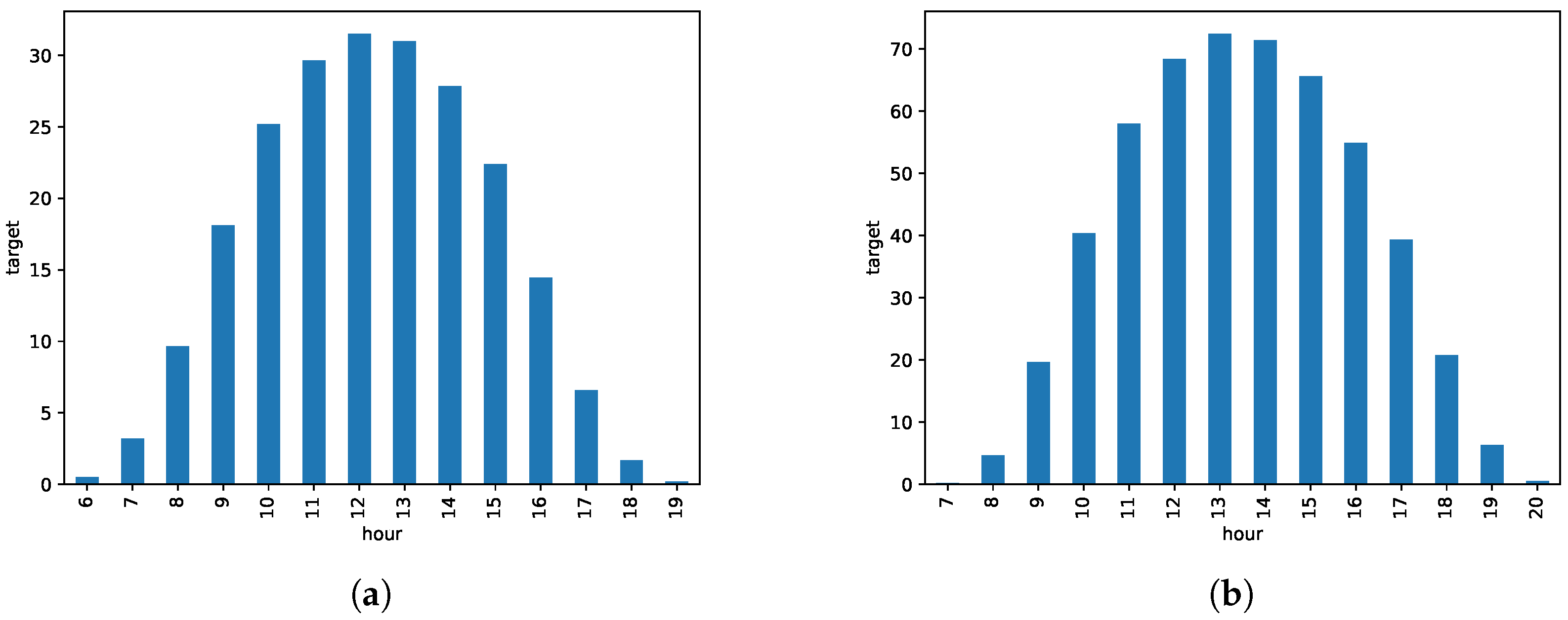
Recall that we will use data from the 2013 year as the training set, 2014 as the validation set, and 2015 for testing. We will give the errors in both $\mathrm{M}\mathrm{W}\mathrm{h}$ and as percentages in the range $[0,100]$ of the total installed PV power at each island, namely, $72.46$ $\mathrm{M}$$\mathrm{W}$ in majorca and $107.68$ $\mathrm{M}$$\mathrm{W}$ in tenerife. For obvious reasons, we will not consider night data and predict solar energy only between 06 $\mathrm{UTC}$ and 19 $\mathrm{UTC}$ for majorca and between 07 $\mathrm{UTC}$ and 20 $\mathrm{UTC}$ for tenerife. The hour of the day has an obvious influence on solar radiation, and the same is true about which period of the year is considered. This leads directly to two different tasks:

• Task by hour: We consider the prediction at each hour as a different task; we have thus 14 tasks in majorca (from 06 to 19 $\mathrm{UTC}$) and tenerife (from 07 to 20 $\mathrm{UTC}$).
• Task by season: We consider four different season tasks which, with a small abuse of language, we will call Spring, from 16 February to 15 May; Summer, from 16 May to 15 August; Autumn, from 16 August to 15 November; and Winter, from 16 November to 15 February.

Figure 1a,b shows the hourly averages in $\mathrm{M}\mathrm{W}\mathrm{h}$ of the PV energy for majorca and tenerife, respectively, and Figure 1c,d shows the seasonal averages by month in majorca and tenerife, colored by season.

4.2.2. Experimental Results

In

Table 2. Test MAEs (left), test MSEs (center), and optimal mixing ${\lambda }^{*}$ (right) of the solar energy models considered in majorca. Base units are either $\mathrm{M}\mathrm{W}\mathrm{h}$ or percentages (%). The best model errors are shown in bold.

	MAE			MSE			${\mathit{\lambda }}^{*}$
	MWh	%	Rank	MWh	%	Rank
ctlSVR	5.265	7.265	(6)	59.322	112.985	(6)	-
(season)_itlSVR	5.305	7.384	(7)	59.591	113.498	(7)	-
(season)_mtlSVR	4.884	6.740	(1)	53.222	101.366	(2)	0.4
(hour)_itlSVR	5.083	7.015	(4)	54.540	103.877	(3)	-
(hour)_mtlSVR	4.957	6.840	(2)	52.614	100.208	(1)	0.3
(hour, season)_itlSVR	5.250	7.251	(5)	57.927	110.328	(5)	-
(hour, season)_mtlSVR	5.038	6.952	(3)	54.601	103.992	(4)	0.3

and

Table 3. Test MAEs (left), test MSEs (center), and optimal mixing ${\lambda }^{*}$ (right) of the solar energy models considered for tenerife. Base units are either $\mathrm{M}\mathrm{W}\mathrm{h}$ or percentages (%). The best model errors are shown in bold. The positions with hyphens correspond to the model ranked first in terms of MAE or MSE, as indicated by its column.

	MAE			MSE			${\mathit{\lambda }}^{*}$
	MWh	%	Rank	MWh	%	Rank
ctlSVR	5.786	5.373	(5)	88.323	76.174	(5)	-
(season)_itlSVR	5.930	5.545	(6)	97.454	84.611	(6)	-
(season)_mtlSVR	5.579	5.181	(4)	86.227	74.366	(3)	0.8
(hour)_itlSVR	5.403	5.018	(2)	86.686	74.762	(4)	-
(hour)_mtlSVR	5.376	4.993	(1)	84.207	72.624	(1)	0.7
(hour, season)_itlSVR	6.025	5.554	(7)	104.536	90.297	(7)	-
(hour, season)_mtlSVR	5.494	5.102	(3)	85.440	73.687	(2)	0.7

, we present the test results for majorca and tenerife. We give both the Mean Absolute Error (MAE), which is the natural score for SVR and energy deviations, as well as the MSE score; the numbers in parentheses show the model rankings according to either the MAE or MSE values. These rankings show that the MTL models obtain the smallest MAE and MSE scores. To analyze their statistical significance, we report in

Table 4. Wilcoxon p-values for absolute (left) and quadratic (right) errors.

	MAE		MSE
	majorca	tenerife	majorca	tenerife
ctlSVR	0.014 (4)	0.000 (5)	0.081 (4)	0.000 (5)
(season)_itlSVR	0.008 (5)	0.636 (5)	0.215 (4)	0.354 (5)
(season)_mtlSVR	—— (1)	0.000 (4)	0.036 (2)	0.000 (3)
(hour)_itlSVR	0.693 (2)	0.006 (2)	0.000 (3)	0.000 (4)
(hour)_mtlSVR	0.067 (1)	—— (1)	—— (1)	—— (1)
(hour, season)_itlSVR	0.000 (3)	0.000 (6)	0.000 (4)	0.098 (5)
(hour, season)_mtlSVR	0.000 (2)	0.000 (3)	0.745 (3)	0.000 (2)

the Wilcoxon test p-values computed pair-wise between the absolute error distributions of a given model and the one following it according to the MAE/MSE rankings in Table 2 and Table 3. Table 4 also shows a model ranking but now in terms of statistical significance; here two models have different rankings if the difference in their error distributions is significant according to the Wilcoxon test at the $0.05$ level. In other words, when we have a value $p<0.05$, we reject the null hypothesis of the distributions of two consecutively MAE/MSE ranked models being the same; thus, each new $p<0.05$ implies a change on these Wilcoxon rankings. On the other hand, when two models are not significantly different, they receive the same ranking. The results in Table 4 show that the (hour)_mtlSVR is the best model for tenerife in terms of both MAE and MSE score, and the best model for majorca by MSE; the best MAE model is now (season)_mtlSVR but its difference with (hour)_mtlSVR is not relevant at the $0.05$ (it would be so at the $0.1$ level). While in majorca both the season and hour task definitions are helpful, it seems, however, that their combination does not improve the individual MTL model results. In Table 2 and Table 3, we also give the optimal values of the $\lambda$ parameter obtained for the multi-task models. We observe that in majorca and tenerife the obtained values show a substantial multi-task behavior, as the optimal ${\lambda }^{*}$ lie clearly away from the 0/1 extremes. However, in majorca these values are closer to 0, which reflects a stronger independent component, while in tenerife, they are closer to 1, which reflects a stronger common component. The persistence forecasts are computed by predicting for a given day and hour the PV energy produced in the same hour of the previous day; the errors for majorca and tenerife are $5.776$ $\mathrm{M}$$\mathrm{W}$$\mathrm{h}$ and $7.766$ $\mathrm{M}$$\mathrm{W}$$\mathrm{h}$, which scaled to $[0,100]$ correspond to 7.97% and 7.21%; these are an 18% and 44% error increase of the best proposed models. The multilayer perceptrons errors are $5.140$ $\mathrm{M}$$\mathrm{W}$$\mathrm{h}$ and $5.763$ $\mathrm{M}$$\mathrm{W}$$\mathrm{h}$, that is, 7.09% and 5.35% of the total PV installed. While competitive, these models’ performances are worse than those of the models proposed in this work.

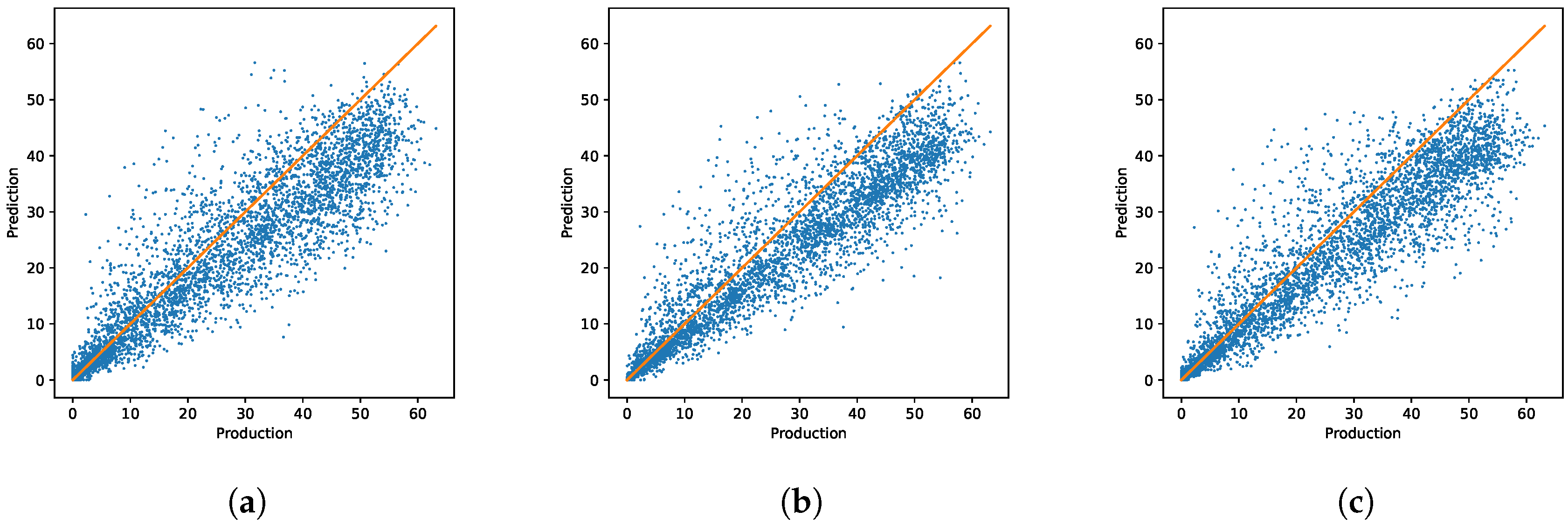
In Figure 2, we plot for majorca test targets against the predictions of the CTL model, the best ITL model according to MAE ((hour)_itlSVR), and the best MAE MTL model ((season)_mtlSVR). Here, we can see that the CTL predictions appear as the most scattered ones, and the ITL predictions are more compact but seem to underestimate production. The MTL approach obtains a more compact model than the CTL one, with less bias than the ITL model.

For tenerife, the hour tasks clearly give the best results for both MTL and ITL models. In Figure 3, we plot once more test targets against the predictions of the CTL model and of the best hourly ITL and MTL models. Now it is more difficult to visually differentiate model performance, although it seems that that the ITL and MTL models outperform the CTL model at the extremes of very large or very small production. This is likely to be due to the specificity of the MTL and ITL models in these small and large production tasks.

4.3. Wind Energy Experiments

4.3.1. Data and Tasks

The goal here is to predict the hourly energy production in the Sotavento wind farm in Galicia, Spain. We will use as predictors the following NWP variables.

• Eastward component of the wind at 10 m (U10).
• Northward component of the wind at 10 m (V10).
• Module of velocity of the wind at 10 m.
• Eastward component of the wind at 100 m (U100).
• Northward component of the wind at 100 m (V100).
• Module of velocity of the wind at 100 m.
• Surface Pressure (sp).
• 2 m temperature (2t)

We will use a grid approximately centered at the farm, with northeast and south-est coordinates being $(-{9.5}^{\circ },{44}^{\circ })$ and $(-6^{\circ },{42.25}^{\circ })$, respectively; resolution here is also ${0.125}^{\circ }$. This results in a 435 point grid and, using 8 different variables at each point, gives a total of 3480 predictive features. We also scale here actual productions to a $[0,100]$ range, with 100 corresponding to the farm rated power ($17.56$ $\mathrm{M}$$\mathrm{W}$). Now, we use the year 2016 for training, 2017 for validation, and 2018 for test. Task definition is not as clear-cut here as it was for solar energy. Nevertheless, we will consider three different task definition criteria.

• Task by angle: Here, we consider the wind angle at 100 $\mathrm{m}$ derived from the U100 and V100 NWP variables. To define 4 different tasks we first estimate the most frequent angle, which has a value of ${56}^{\circ }$ and we take it as the center of a first ${90}^{\circ }$ sector. This sector defines the first task and the three other tasks are in turn defined by the remaining ${90}^{\circ }$ sectors. These sectors as well as the angle histograms are shown in Figure 4a.
• Task by velocity: We consider here three different tasks attending at the distribution of the wind speed at 100 $\mathrm{m}$ in relation to the energy produced, as shown in Figure 4b. We choose the boundary speeds to be 4 and 10 $\mathrm{m}$/$\mathrm{s}$, which approximately match, for an ideal aerogenerator, the starting of wind energy generation and its maximum power plateau before the cut-off speed.
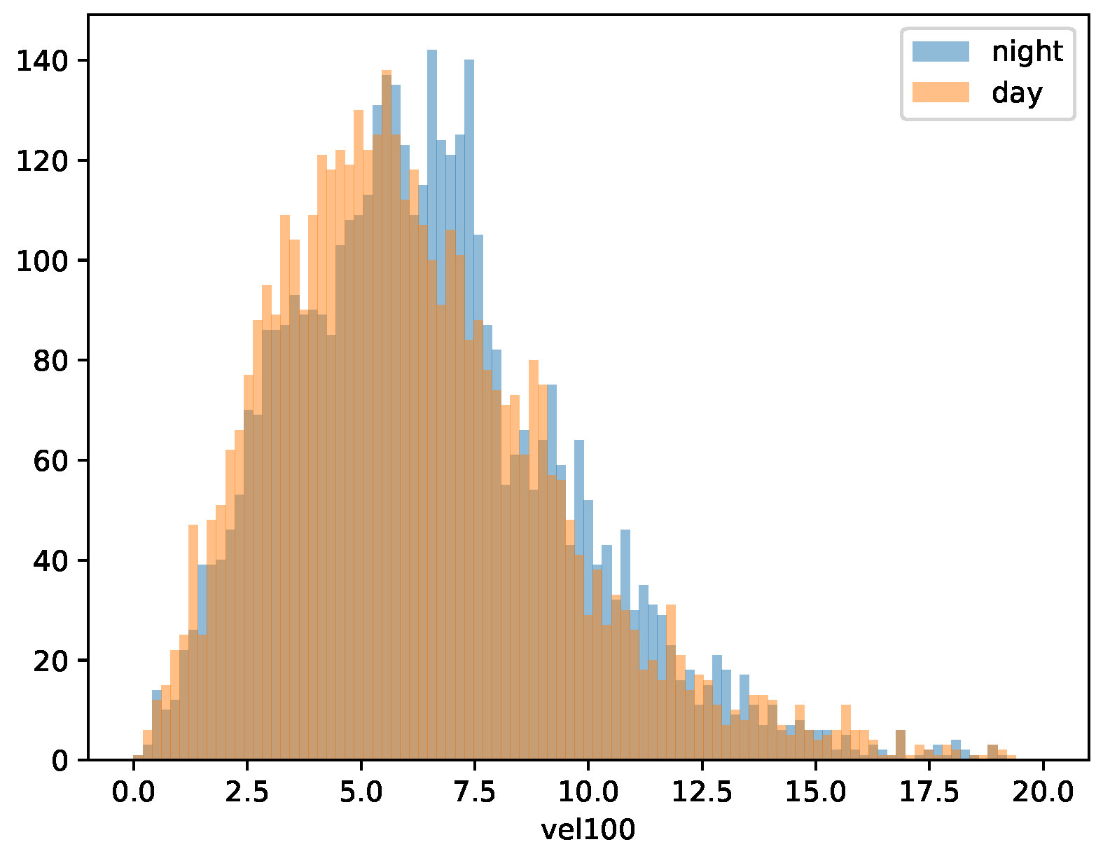
• Task by timeOfDay: Here we divide the day in two parts, namely, a day period between 08 and 19 $\mathrm{UTC}$, and a night one between 20 to 07 $\mathrm{UTC}$, which results in two periods of 12 h. In Figure 5a, we can see the hourly energy mean colored using this task definition. Moreover, in Figure 5b we can observe the hourly mean of wind velocity (at 100 $\mathrm{m}$) colored by task definition timeOfDay, as well as the histograms of the wind velocity during the two time periods defined by timeOfDay in Figure 6.

To define the different tasks we only use data from the training set, that is, data from 2016. As mentioned, wind energy behavior does not have task profiles as clear-cut as those for solar energy. In the case of tasks angle and velocity, there exist differences among tasks in the histograms; however, it is not clear where to draw the line that separates one task from the other, and a bad selection of this separation could lead to poor performance. Moreover, the task timeOfDay does not show marked differences between the night and day tasks velocity distributions, as it can be observed in Figure 6.

4.3.2. Experimental Results

The MAE and MSE scores are shown in

Table 5. Test MAEs (left), MSEs scores (center), and optimal mixing ${\lambda }^{*}$ (right) of the Sotavento wind energy models considered. The best model errors are shown in bold.

	MAE	MSE	${\mathit{\lambda }}^{*}$
ctlSVR	6.132 (1)	90.228 (2)	-
(velocity)_itlSVR	6.211 (7)	93.363 (7)	-
(velocity)_mtlSVR	6.208 (6)	93.199 (6)	0
(timeOfDay)_itlSVR	6.283 (9)	93.594 (9)	-
(timeOfDay)_mtlSVR	6.132 (1)	90.228 (2)	1
(timeOfDay, velocity)_itlSVR	6.341 (11)	97.250 (11)	-
(timeOfDay, velocity)_mtlSVR	6.312 (10)	94.774 (10)	0.4
(timeOfDay, angle)_itlSVR	6.266 (8)	93.517 (8)	-
(timeOfDay, angle)_mtlSVR	6.132 (1)	90.228 (2)	1
(timeOfDay, angle, velocity)_itlSVR	6.410 (12)	102.031 (12)	-
(timeOfDay, angle, velocity)_mtlSVR	6.132 (1)	90.228 (2)	1
(angle)_itlSVR	6.170 (4)	91.586 (4)	-
(angle)_mtlSVR	6.135 (2)	90.026 (1)	0.9
(angle, velocity)_itlSVR	6.173 (5)	92.529 (5)	-
(angle, velocity)_mtlSVR	6.168 (3)	90.990 (3)	0.7

; again, the numbers in parentheses show model rankings, increasing for both MAE and MSE. We first observe that the ctlSVR approach in this problem obtains much better results than those of any itlSVR model. This difference is probably due to the wind energy behavior which, as mentioned and in contrast with the PV situation, is not as clear-cut across tasks as it was in the case of solar energy. Thus, the corresponding wind task definitions do not appear to be highly discriminative. Moreover, and as seen in the table, the (timeOfDay)_mtlSVR, (timeOfDay, angle)_mtlSVR, and (timeOfDay, angle, velocity)_mtlSVR models have an optimal value of $\lambda =1$, i.e., they reduce to the ctlSVR model. All of them give the smallest MAE values, with that of the (angle)_mtlSVR model a close second; observe that it also has a high $\lambda =0.9$ value. On the other hand, the smallest MSE value is that of (angle)_mtlSVR, followed closely now by that of the ctlSVR model and their equivalent MTL models. As for the other MTL models, (angle, velocity)_mtlSVR and (velocity)_mtlSVR have MAE values close to that of (angle)_mtlSVR but larger values of MSE; in all cases, (timeOfDay, velocity)_mtlSVR falls clearly behind. The persistence forecasts for a given day and hour are again the previous day’s energy at the same hour. Its error is a quite large $15.63\%$, a $150\%$ increase on the error of the best model. This is to be expected as there is very little correlation of wind energy values 24 h apart, in contrast with what happens with solar energy. The multilayer perceptron obtains an error of $6.66\%$, also greater than any of the SVM models presented here.

For a more precise analysis,

Table 6. Wilcoxon p-values and corresponding ranking for absolute (right) and quadratic (left) wind energy errors in Sotavento. The positions with hyphens correspond to the model ranked first in terms of MAE or MSE, as indicated by its column.

	MAE	MSE
ctlSVR	—— (1)	—— (2)
(velocity)_itlSVR	0.570 (3)	0.150 (3)
(velocity)_mtlSVR	0.356 (3)	0.466 (3)
(timeOfDay)_itlSVR	0.195 (4)	0.258 (4)
(timeOfDay)_mtlSVR	—— (1)	—— (2)
(timeOfDay, velocity)_itlSVR	0.941 (4)	0.021 (5)
(timeOfDay, velocity)_mtlSVR	0.428 (4)	0.650 (4)
(timeOfDay, angle)_itlSVR	0.000 (4)	0.015 (4)
(timeOfDay, angle)_mtlSVR	—— (1)	—— (2)
(timeOfDay, angle, velocity)_itlSVR	0.090 (4)	0.024 (6)
(timeOfDay, angle, velocity)_mtlSVR	—— (1)	—— (2)
(angle)_itlSVR	0.855 (3)	0.644 (3)
(angle)_mtlSVR	0.035 (2)	—— (1)
(angle, velocity)_itlSVR	0.253 (3)	0.465 (3)
(angle, velocity)_mtlSVR	0.018 (3)	0.001 (3)

gives Wilcoxon p values at the 0.05 level obtained when we compare each model with the next one according to the MAE and MSE rankings shown in Table 5. As it can be seen, when MAEs are considered, the ctlSVR obtains the first place tied, of course, with the (timeOfDay)_mtlSVR, (timeOfDay, angle)_mtlSVR and (timeOfDay, angle, velocity)_mtlSVR models; (angle)_mtlSVR occupies now the second place, and these roles are reversed when considering MSE values, with (angle)_mtlSVR being significantly first. Recall that rankings change when for two MAE or MSE consecutive models we have a value $p<0.05$, while when they are not significantly different, the models receive the same ranking. Now the (angle, velocity)_mtlSVR and (velocity)_mtlSVR model tie with (angle)_mtlSVR for second place when MAE values are considered but fall to third and fifth places, respectively, for MSE; here again (timeOfDay, velocity)_mtlSVR is clearly worse.

As we did for PV energy, in Figure 7 we plot test targets against the predictions of the CTL model, of the best hourly ITL model (angle)_itlSVR, and of the best pure MTL model (angle)_mtlSVR; visual differentiation is now much less clear. We also point out the presence of points with a zero production and large predictions, something relatively frequent in wind energy, either because of energy curtailments or because periods in which the wind farm is under maintenance, and therefore stopped, may coincide with substantial winds. Notice also the stronger presence of small production values below 20%, something due to the approximate Weibull distribution of wind speeds, which gives higher frequencies to small speed values; this also makes it difficult to visually appreciate the differences between model performance.

We finally observe that while the wind MAEs in percentage are similar to those in PV, when compared with the energy produced, the performance of wind models is actually worse. In fact, in

Table 7. Comparison of the percentage MAEs with the average energy produced as a percentage of installed power.

	MAE (%)	Avg. Target (%)	Ratio
majorca	6.740	29.954	22.50
tenerife	4.993	33.462	14.92
sotavento	6.186	17.784	34.78

we compare the percentage MAE against the average generated energy as a percentage of installed power. As it can be seen, the ratio between the percentage MAE and the percentage average energy is about $34.78\%$ for Sotavento, much higher than the $22.50\%$ of Majorca and the $14.92\%$ of Tenerife.

4.4. Considerations on Computational Costs

In general, there are two costs when building machine learning models. The first is that of the hyperparameter tuning process; this is in general quite costly, as many different hyperparameter combinations have to be tried before choosing the optimal one. However, this is usually done just once, before models go into exploitation. What is more important from the model exploitation and maintenance point of view is, once the best hyperparameters are chosen, the computational effort needed to train and retrain when needed the model being used. Notice that for SVR-based models the training effort depends essentially on two inputs:

• Sample size, as it is well known that SVM training cost is at least quadratic with respect to the number of samples. Moreover, recall that, in our case, we precompute the kernel matrix before training starts, and sample size also impacts here. In particular, the MTL kernel matrix has two components: the standard kernel matrix of the global CTL model plus the component derived from the independent models; thus, the MTL cost here should be larger than the CTL cost.
• The hyperparameters being used and, particularly, the value of C, as it bounds the dual multipliers and a large C implies a large area to be explored during training and, therefore, an often large training time.
  To C we may add the $ϵ$ hyper-parameter, which also affects training time, as small values imply more precise and, therefore, possibly costlier to train models. However, as far as we know, its impact in training times (as well as that of the kernel width) is more difficult to quantify.

Sample size (and thus the dimension of the dual space where our SMO solver works) is the same for the CTL and MTL models, as they work on the entire sample. Therefore, in principle and after the corresponding kernels are computed, their complexity and training costs should be similar, although training times may vary as they may use different C and $ϵ$ hyper-parameters. On the other hand, sample size of the ITL models may be much smaller. For instance, in the solar case, sample size are 4 times smaller when tasks are defined by the 4 seasons we consider, 14 times smaller when tasks are defined by the 14 h we consider and, finally, 56 times smaller when both are combined. Of course, this is balanced by the correspondingly larger number of models to be trained: for instance, we need to train 56 ITL models for the hour–season task combination. This is a lot of models but, however, this training can be done largely in parallel fashion, which can substantially lower response time. Thus, ITL training complexity is not comparable with that of the CTL and MTL models, and should be clearly lower. In summary, we should expect CTL training times to be slightly smaller than those of MTL, and the ITL times to be clearly smaller.

With these considerations taken into account, a comparative of the training times of the best models can be found in

Table 8. Training time in seconds of the CTL and best ITL and MTL models for each problem.

	CTL	ITL	MTL
majorca	9.56	6.92	11.77
tenerife	14.08	7.48	17.52
sotavento	86.01	53.20	82.96

. The time is measured using the function process_time() from the library time. Recall that the best ITL and MTL models for majorca use the (hour) and (season) task definitions, respectively. For tenerife, both the best MTL and ITL models correspond to (hour) task definition. In stv, the best ITL and MTL models are (angle) and (timeOfDay, velocity) task definitions, respectively. As it can be seen, the measured training times roughly follow what can be expected from the previous discussion. We point out that the ITL times correspond to training them in an iterative fashion; if done in parallel, total ITL time would be much smaller. Finally, we notice that, while not negligible, training times are not exaggeratedly large and would fall well within operation requirements.

5. Conclusions

Accurate predictions of renewable energy production are becoming mandatory nowadays because of the high impact of this type of energy. Machine learning (ML) offers a useful tool in this context, allowing to estimate the future energy production using as input information numerical weather predictions (NWPs). In this context, multitask learning (MTL) aims to improve the performance over several related ML problems (called tasks) by exploiting their similarities, and at the same time allowing for certain independence between them.

In this work, we have applied support vector regression (SVR)-based MTL models to two photovoltaic (PV) energy problems and a wind energy one. Our SVR-MTL models are intermediate between a global SVR model, which we refer as CTL and works over all tasks, and a set of independent task models, one per task, which we collectively refer as the ITL model. A parameter $\lambda \in [0,1]$ gives a bigger or smaller emphasis to one of these extreme models. In our formulation, the SVR-MTL model reduces to CTL when $\lambda =1$; in a more general formulation than the one we use, the SVR-MTL model would reduce to the ITL one when $\lambda =0$, but this is not the case here, as we introduce some simplifications to the more general MTL set-up in order to apply the well-known SMO solver for SVR training. Task definition is more clear-cut in the solar case, as the hour of the day and the season have a strong influence in the production of PV energy. Moreover, PV tasks can be defined without using the prediction features. In contrast, while sensible tasks can in principle be defined for wind energy, their effect in actual energy production is less direct, either because we have to rely on NWP forecasts, with their inherent imprecision, to define the tasks or because the day–night tasks, which we also consider, depend on boundary layer effects which, while true in general, may depend substantially on local wind farm conditions.

This is reflected in our results. For wind energy, the best results are given by the CTL model, to which several MTL models reduce as they select $\lambda =1$ as the optimal value for the mixing parameter. In other words, task differentiation does not help to get better results in our wind problem. On the other hand, if only MTL models were used, they would also yield the global CTL model as their best results. Thus, here MTL models do not hamper the search for the best model. The situation is very different, however, for the Majorca and Tenerife PV problems. As mentioned, task differentiation is much clearer here, and it results in two MTL models yielding the best results, very clearly in the more difficult Majorca problem and in a less marked but still statistically significant way for the easier (because of the more stable and sunny weather) Tenerife problem.

In any case, there is room for improvement. A first area is that of model hyperparametrization. While the CTL and ITL models have the three SVR—C, $ϵ$, and $\gamma$—hyperparameters, more options are available for MTL models. For instance, for the MTL models we only hyperparametrize here C, $ϵ$, and $\lambda$, and we use the $\gamma$ kernel widths that are optimal for the CTL and MTL models; it is thus conceivably that MTL performance may be enhanced by a more specific choice of kernel widths. Similarly, we just use a single common $\lambda$ for all tasks, but our SVR-MTL proposal can also handle task specific $\lambda$ values. These two options open a way to further improve MTL performance in a way that is precluded for the CTL and ITL counterparts, although, of course, with a possibly much greater hyperparametrization effort (on the other hand, we have illustrated how training times for CTL and MTL models are fairly similar). We are currently considering how to tackle this, where probabilistic points of view can help, either in a simple random exploration of the hyperparameter space or through a more focused Bayesian search.

Another area for improvement is to consider ways to allow the tasks to interact with each other. In our current formulation, they behave more or less independently, being only indirectly connected through the common model. This could be corrected, for instance, by considering the distances between the ITL models and somehow enforce that similar tasks are served by close models while leaving more leeway for models acting on distant tasks. Another obvious way is to look for new approaches to divide the problem into tasks from two different perspectives, either using expert knowledge to see which other factors can change significantly the production behavior, or using automatic tools for grouping data that behaves similarly following a (possibly semisupervised) clustering approach. Finally, another interesting role MTL models can play in energy prediction is to consider on an MTL set-up wind or solar energy of farms that are relatively close and which would define the individual tasks. Here, the global model could capture overall atmospheric conditions that may affect all farms, and each individual task could reflect more farm-specific effects. We are currently working on these ideas.