Water Conservation Potential of Self-Funded Foam-Based Flexible Surface-Mounted Floatovoltaics

Abstract

A potential solution to the coupled water–energy–food challenges in land use is the concept of floating photovoltaics or floatovoltaics (FPV). In this study, a new approach to FPV is investigated using a flexible crystalline silicon-based photovoltaic (PV) module backed with foam, which is less expensive than conventional pontoon-based FPV. This novel form of FPV is tested experimentally for operating temperature and performance and is analyzed for water-savings using an evaporation calculation adapted from the Penman–Monteith model. The results show that the foam-backed FPV had a lower operating temperature than conventional pontoon-based FPV, and thus a 3.5% higher energy output per unit power. Therefore, foam-based FPV provides a potentially profitable means of reducing water evaporation in the world’s at-risk bodies of fresh water. The case study of Lake Mead found that if 10% of the lake was covered with foam-backed FPV, there would be enough water conserved and electricity generated to service Las Vegas and Reno combined. At 50% coverage, the foam-backed FPV would provide over 127 TWh of clean solar electricity and 633.22 million m³ of water savings, which would provide enough electricity to retire 11% of the polluting coal-fired plants in the U.S. and provide water for over five million Americans, annually.

1. Introduction

Water scarcity [1,2], the energy crisis [3], and food scarcity [4,5] are the largest currently coupled challenges [6] facing the global community, where they most severely affect the arid and semiarid regions of the world [7]. There is a wide scientific consensus that combustion of fossil fuels for energy is increasing atmospheric carbon dioxide (CO₂) concentrations and driving climate change [8]. This anthropogenic climate change is increasing globally averaged mean annual air temperatures and driving changes in precipitation, which are expected to continue and increase [9,10]. The IPCC (Intergovernmental Panel on Climate Change) warns that the climate change over the next century will affect rainfall, river flows and sea levels all over the world [11], which will negatively impact agricultural yield [12]; particularly in already-malnourished sub-Saharan Africa. de Wit and Stankiewicz [13] predict rainfall in sub-Saharan Africa could drop by 10% causing surface drainage to drop 30–50% by midcentury, which would cause major water shortages. It is widely agreed that to prevent the worst of climate change, humanity needs to rapidly convert fossil fuel-based energy systems to renewable energy systems [14]. Solar photovoltaic (PV) technology is the most widely accessible, sustainable, and clean renewable source of energy that can be scaled to meet humanity’s energy needs [15,16]. To meet these needs, however, a substantial amount of land is still needed for PV to replace fossil fuels and this creates competition for limited land resources between food and energy [17]. A utility-scale PV plant land occupation varies between 20 km²/GWh and 40 km²/GWh depending on the type of solar panels used [18]. Despite life cycle carbon emissions [19], PV is more land efficient than all carbon capture and sequestration plans for coal [20], but with nearly a billion people already living undernourished, further reductions in agricultural land are not acceptable during a world food crisis [21].

A potential solution to these coupled water–energy–food challenges is the concept of floating photovoltaics or floatovoltaics (FPV), which has been rapidly gaining a base in scientific literature [22,23,24,25,26,27,28]. FPV is growing fast and is expected to have an average growth rate of above 20% in the next five years due to extremely low costs (with an FPV bid recently coming in for a system in Thailand at under USD 0.50/Wp) [29]. FPV are easier to install and simpler to decommission than conventional PV systems and the racking costs are less, which lead to these overall cost savings [29]. As FPV are located near or immersed in water, the operational temperature is reduced, which raises the solar energy conversion efficiency [23,26,30,31,32,33,34]. In regions where water scarcity is an issue and particularly when this issue is likely to be aggravated by climate change, FPV can also be used to reduce water loss because it can reduce water evaporation by more than 70% [32,35,36,37]. The Penman–Monteith daily evaporation method indicates that FPV could even cut evaporation by as much as 90% [38]. Studies in China [39] and India [40,41] have all indicated massive potential water savings for both small and large FPV coverage areas. This is particularly important for preservation of water sources in arid and semi-arid regions, especially with water shortages in the region [42]. FPV, therefore, also holds substantial promise when coupling with existing hydro power to make dual use of the electrical infrastructure while improving the water resource itself [39,43]. Similar advantages are to be expected for hybrid systems with pumped storage [44]. Finally, there is also evidence that FPV deployment reduces the PV degradation rate below 0.5% per year [45], which improves the levelized cost of solar electricity further.

FPV research has focused on several system design strategies [46]:

(1)

Tilted arrays of solid modules (normally on top of pontoon structures) [36,47,48,49];

(2)

Submerged PV modules (with and without a pontoon) [24,30,33,34,50];

(3)

Micro-encapsulated phase change material (MEPCM)-based pontoon modules [51,52,53];

(4)

Thin-film PV (no ridged pontoon supporting structure) [24,26,54].

The thin-film FPV design has the advantage of reducing racking costs even more so than pontoon style FPV, as it clearly stops more evaporation and gains an advantage by the operational temperature being lower. However, the temperature coefficients are better for amorphous silicon (a-Si:H) thin film materials than those of crystalline silicon (c-Si) so the benefits of the water cooling are muted for a-Si:H-based FPV.

In this study, a new approach is used with a flexible crystalline silicon module on a similar foam system to that described by Pierce et al. [54] for a-Si:H FPV. This approach enables a larger solar electric output gain (or FPV boost) and as solar is largely already profitable, there is an opportunity for the electricity production value of c-Si flexible foam-backed FPV to subsidize a means of water conservation by cutting water evaporation losses. To build on past FPV work and investigate the potential of FPV coupled to hydro power in the U.S., the water saving potential at Lake Mead using FPV is investigated in this study. Lake Mead is an artificial reservoir created by the United States government to run the Hoover Dam, which was built in 1935 [55,56]. This novel form of FPV is analyzed for water-saving using an evaporation calculation adapted from the Penman–Monteith daily evaporation model [57] that is approved by the Food and Agriculture Organization of the United Nations (FAO) [58]. An energy production analysis is performed and an open source spreadsheet was developed to simulate the evaporation and the energy yield of the flexible FPV [59], as well as to investigate the impact of using passive water-cooled FPV, where the cooling potential was measured experimentally for a foam-based FPV. The potential is determined for a case study based on the coverage of FPV ranging from 10% to 50% [60] of Lake Mead. The results are compared to “conventional” tilted pontoon-style FPV and are discussed in the context of the energy–water–food nexus.

2. Materials and Methods

2.1. Data Collection

2.1.1. Lake Evaporation Data

Most of the weather data used in this study were collected on Lake Mead through buoys installed by the United States National Oceanic and Atmospheric Administration’s National Data Buoy Center (NOAA-NDBC) [61]. The rest of the data were obtained from open-access weather data made available by the McCarran International Airport’s weather station in Las Vegas [62], and from SOLCAST, a solar data provider [63].

The main characteristics of the lake differ slightly from one study to another and depend on the year the study was conducted. In this study, the lake characteristics’ values used for the evaporation calculation are taken from the National Park Service (NPS) website [64]. According to the NPS, as of 2010, the lake has a maximum surface area of 159,866 acres (647 million m²), and a maximum capacity of 29,686,054 acre-feet (36,617 million m³). The mean depth of the lake is estimated to be 55.5 m by the National Park Service [56]. The elevation of the lake is 328.574 m above sea water level. The weather buoy used to collect the data is located in the North Boulder Basin of the lake at a geographical position of latitude 36.087 N and longitude 114.728 W. The temperature sensor for air temperature collection is located at a height of 2 m above the lake surface while the anemometer is at 3 m above. Additionally, the atmospheric pressure sensor is located at 330.574 m above sea water level or 2 m above the lake surface, and the water temperature is measured at 0.5 m below the lake surface [65].

The buoy installed in Lake Mead’s North Boulder basin by the NOAA-NDBC has been capturing different types of variables since 2016, which are stored in a historical database on the agency’s website. Among the data required to conduct an evaporation calculation using the Penman–Monteith model, the wind speed (w_s), the atmospheric pressure (P), the maximum (T_w,max), minimum (T_w,min), and daily mean (T_w) water temperature; and the air temperature were obtained from the NOAA-NDBC historical database. The rest of the data were not captured by the buoy; therefore, alternative methods have been used to gather the required data. According to Moreo and Swancar, when data are not available for the study location, nearby airport weather data can be used instead [55]. In this study, the nearest airport close to Lake Mead is the Las Vegas Airport. The relative humidity (Rh) data have thus been obtained from the Weather Underground website that has made data from the Las Vegas Airport available. The remaining variable is the daily incoming solar irradiation or global horizontal irradiation (R_S) that has been obtained from SOLCAST’s historical database [63]. This variable is also used for the solar energy production modeling.

The raw data from the NOAA-NDBC database were collected with an interval of 10 min starting at 00 h 00 min each day while the data from the Las Vegas Airport were measured with an 1 hour interval starting at 00 h 56 min each day. Since daily data were required for the calculation, a mean daily value has been calculated for each variable. First, the data obtained from the NOAA-NDBC were cleaned by keeping only hourly data at the beginning of the hour (00 min) in order to match the data from Las Vegas Airport. A MATLAB code [66] was developed to perform this operation. Then, the same code was used to strip the missing data from the data table. A line of data was considered missing from the data table if one or more of the variables were not recorded by either the NOAA-NDBC station sensors or the Las Vegas Airport station sensors. After that, the data were reported in a spreadsheet that was used to calculate the mean daily value of the wind speed (w_s), the atmospheric pressure (P), the water temperature (T_w) and the air temperature (T_a) by averaging the hourly data for each day. Another method used in the literature to calculate daily mean weather data is to calculate the average of the maximum and minimum value of the day [67]. However, studies have shown that if data are available, it is best to calculate the mean daily temperature by averaging the hourly values [68,69]. The spreadsheet was also used to retrieve the maximum (T_w,max), and minimum (T_w,min) daily temperatures as well as the maximum (Rh_max), and minimum (Rh_min) daily relative humidity. The number of missing data points was 246 hourly data. Instead of having total hourly data of 8760 points, 8514 data points were used for this study after the data cleaning process. There was no more than 3 missing data points for a single day except for 5 specific days that are the 4th, 60th, 97th, 318th, and 347th day of the year 2018. These 5 days were, respectively, missing 4, 4, 10, 5, and 16 data points. The days with the highest number of missing data were the 97th and 347th day of the year. Since there are only two such days among the 365 that populated the year 2018, it has been considered that it will not have a significant impact on the results. Therefore, the available data were representative in estimating the mean daily values of the variables for each day.

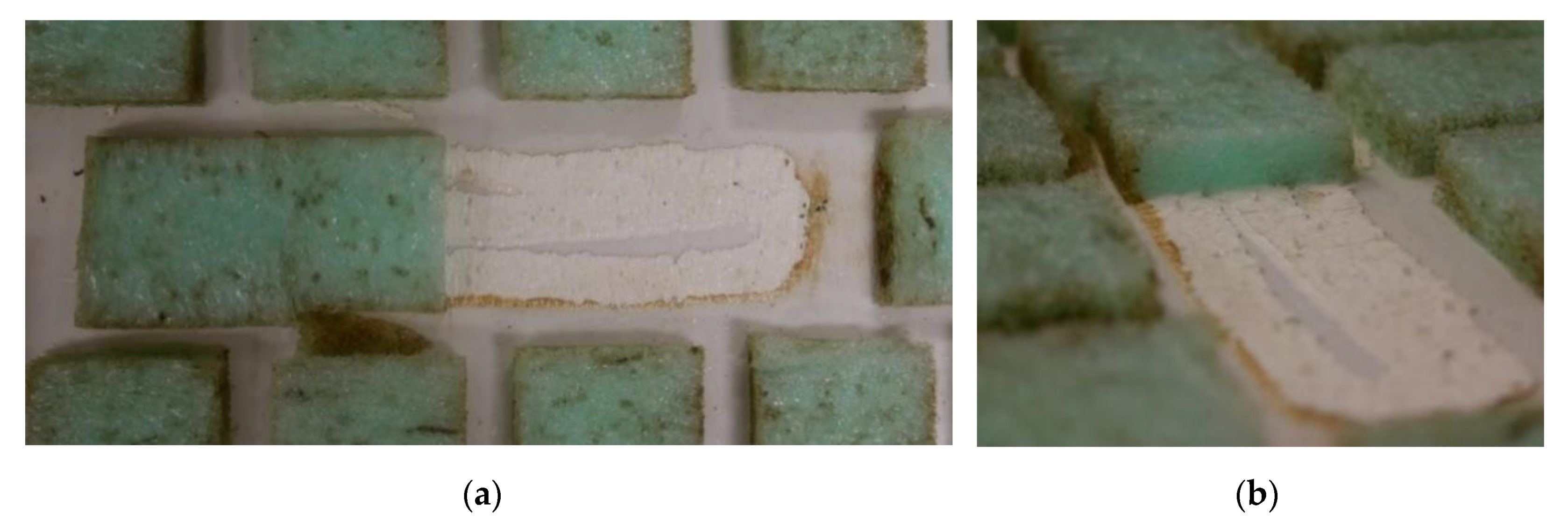
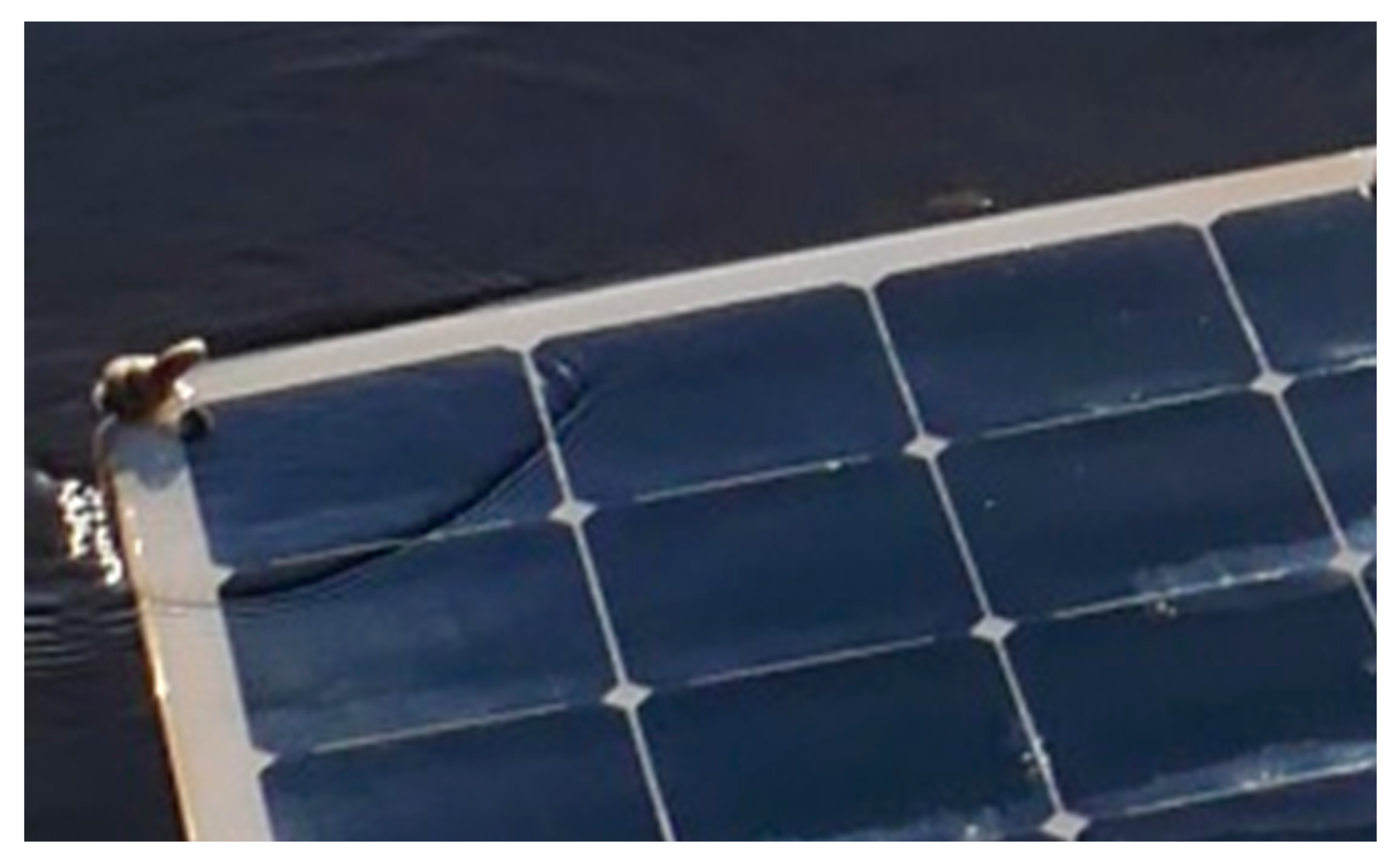
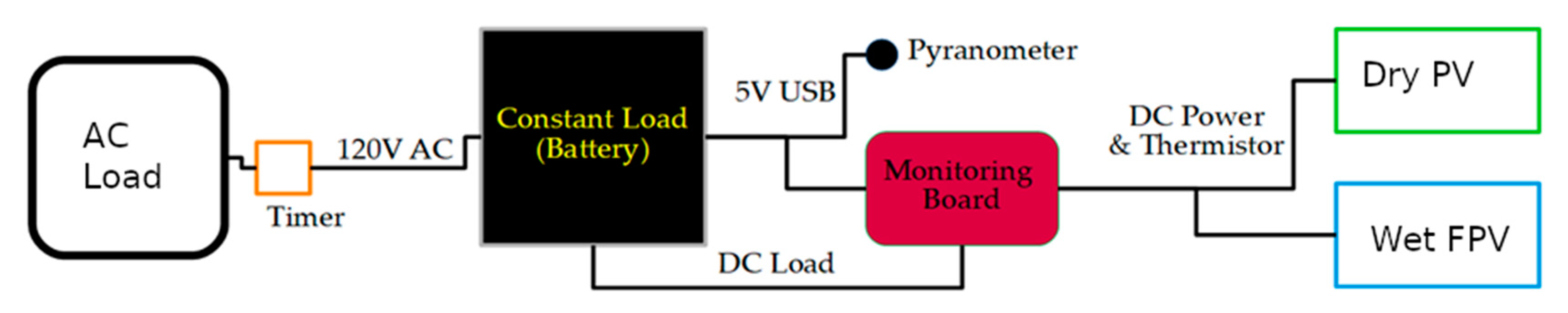
2.1.2. FPV Panel Data Collection

In a previous study, it was found that polyethylene (PE) foam was the most cost-effective way to add buoyancy to flexible solar modules [54]. This study uses this after-market conversion method to convert SunPower SPR-E-Flex PVs into FPVs [70]. The density of the green polyethylene 1.2 lb ½” (12.7 mm) was used to determine the area of foam needed to make the panel rise by approximately 10 mm above the water’s surface [71] using the calculations detailed in [54]. The foam was cut into about 50 mm by 240 mm sections that were placed evenly on the backside of module. The sections were then adhered using 3 M 5200 fast-set waterproof adhesive. Each foam piece had a line of adhesive caulked onto its perimeter and through the center. Then, the foam piece was pressed on the surface of the panel to adhere it, see Figure 1. The FPV with PV control was deployed in Chassell Bay, MI during the summer of 2020 to determine operational temperature and performance. This resulted in the FPV floating directly above the water surface, but still enabling wave action to clear the modules as shown in Figure 2.

The NanoDAQ monitoring board used in [54] was used in this study to measure module power and temperature of both the control (flat land-based mounted dry PV set at zero degree tilt angle) and wet FPV (floating on lake surface). The thermistors used for measuring temperature were held in place on the panels using 3M VHB tape. The air and water temperature were also measured with thermistors. The SunPower panels came with MC4 connectors installed on 12 AWG (2 mm²) wires. MC4 connectors were added to the 14 AWG (1.6 mm²) wires coming from the NanoDAQ, including the load wires. An additional hole was made in the NanoDAQ waterproof case and sealed using 3M 5200 to use the battery’s USB port to power it. An AC load with a timer was used to drain the battery during mid-day to ensure there was a load to produce the power measurement. The schematic of the wiring diagram for the experimental set up is shown in Figure 3.

The FPV utilized mooring similar to that used in [54] except for the inclusion of a buoy. The wet FPV was moored by using an anchor and a towing ring on land. A rope was looped through the grommets in the solar PV and overhand loop knots were tied to secure the FPV in place. Energy generation of dry PV and wet FPV, temperature of air, water, PV, and FPV were recorded in 15 min increments.

2.2. Water Evaporation Modeling

The Penman–Monteith model used in this study is a datum intensive water evaporation model because it requires the measurement of several weather data. Some of the data can be calculated, but the accuracy of the model is increased if they are measured. The Penman–Monteith model was originally designed to calculate the evapotranspiration losses from leaves’ and canopies’ surfaces [57]. However, the method has been adapted in several studies to estimate the evaporation of surface water [72,73,74,75]. One important thing to note regarding the use of the Penman–Monteith evapotranspiration model for lake evaporation is the use of water temperature instead of air temperature in some of the parameters’ calculations: the outgoing longwave radiation, the partial vapor pressure at the water surface and slope of the temperature saturation water vapor curve. The original Penman–Monteith model estimates the evapotranspiration of crops; therefore, the model only uses the air temperature in its implementation. The use of water temperature instead of air temperature has been validated in several lake evaporation studies [72,74,75].

The Penman–Monteith [57] equation adapted to open water surfaces is [74,75]:

$$E_L=\frac{1}{\lambda }\times \frac{\left(\Delta \times \left(R_N-H_S\right)+86400\times {\rho }_a\times C{p}_a\times \raisebox{1ex}{$\left(P_w-P_a\right)$}\!\left/ \!\raisebox{-1ex}{$r_a$}\right.\right)}{\Delta +\gamma } \left(\mathrm{mm}·{\mathrm{day}}^{-1}\right)$$

(1)

where E_L (mm/day) is the daily evaporation rate and Cp_a (kJ/kg/°C) and ${\rho }_a$ (kg/m³) are, respectively, the heat capacity, and the density of air. The other parameters in the Penman–Monteith equation need to be calculated and depend on several weather data. The weather data needed to calculate these parameters are comprised of: the daily maximum (T_a,max) (°C) and daily minimum (T_a,min) (°C) air temperature; the daily maximum (T_w,max) (°C), daily minimum (T_w,min) (°C), and daily mean water temperature (T_w) (°C); the daily maximum (Rh_max) (%), and daily minimum relative humidity (Rh_min) (%); the daily mean dew temperature (T_d) (°C), the daily mean atmospheric pressure (P) (kPa); the daily mean wind speed (w_s) (m/s) at a height of 2 m above the water surface; and the daily incoming solar radiation (R_S) (MJ/m²/day). The other parameters that are needed to calculate the components in the evaporation model of Penman–Monteith include: the altitude of the lake’s location (h) (m); the surface area (A) (m²), and the effective depth (d_w) (m) of the lake reservoir; and the latitude of the location of the water surface $\left(\varphi \right)$ (rad).

When all the listed parameters are available, the computation of the lake water evaporation using the Penman–Monteith model starts with the calculation of the mean saturation vapor pressure (P_w) (kPa), and the actual vapor pressure of the air (P_a) (kPa) [58,67,73]:

$$P_w=\frac{1}{2}\times 0.6108\times \left(\exp \left(\frac{17.27\times T_{w,\mathit{max}}}{T_{w,\mathit{max}}+237.3}\right)+\exp \left(\frac{17.27\times T_{w,\mathit{min}}}{T_{w,\mathit{min}}+237.3}\right)\right) \left(\mathrm{kPa}\right)$$

(2)

$$\begin{array}{ll}{P}_a=\frac{1}{2}\times 0.6108& \times (\frac{R{h}_{min}}{100}\times \exp \left(\frac{17.27\times T_{w,max}}{T_{w,max}+237.3}\right)+\frac{R{h}_{max}}{100}\\ & \times \exp \left(\frac{17.27\times T_{w,min}}{T_{w,min}+237.3}\right)) \left(\mathrm{kPa}\right)\end{array}$$

(3)

After the calculation of the two vapor pressures, the slope of the saturation vapor pressure curve (Δ) (kPa/°C) is calculated [58,67,73]:

$$\Delta =\frac{4096\times P_w}{{\left(T_w+237.3\right)}^2} \left(\mathrm{kPa}·°{\mathrm{C}}^{-1}\right)$$

(4)

Then, the latent heat of vaporization (λ) (MJ/kg), which depends on the water temperature, is calculated [58,73]:

$$\lambda =2.501-0.002361\times T_w \left(\mathrm{kPa}·°{\mathrm{C}}^{-1}\right)$$

(5)

From the latent heat of vaporization, the psychrometric constant (γ) (kPa/°C) can be deduced [58,67],

$$\gamma =\frac{C{p}_a\times P}{R_{MW}\times \lambda } \left(\mathrm{kPa}·°{\mathrm{C}}^{-1}\right)$$

(6)

In Equation (6), R_MW = 0.622 and is equal to the molecular weight of water vapor over the molecular weight of dry air.

After that, the wind function f_w (MJ/m²/kPa/day) is needed to estimate the aerodynamic resistance of the water surface. The formula used to calculate the wind function is proposed by McJannet et al. [76]. The formula was found to work well with the Penman–Monteith evaporation model. The wind function calculation by McJannet’s formula depends on the wind speed as well as on the surface area of the lake.

$$f_w=\left(2.36+1.67\times w_s\right)\times A^{-0.05} \left(\mathrm{MJ}·{\mathrm{m}}^{-2}·{\mathrm{kPa}}^{-1}·{\mathrm{day}}^{-1}\right)$$

(7)

Once the wind function is known, a combination of the Penman–Monteith model equations presented in the works of Zotarelli et al. and Finch et al. gives the value of the aerodynamic resistance (s/m) [67,75]:

$$r_a=\frac{{\rho }_a\times C{p}_a\times 86400}{1000\times \gamma \times f_w} \left(\mathrm{s}·{\mathrm{m}}^{-1}\right)$$

(8)

The two remaining terms are the net solar radiation (R_N) (MJ/m²/day) and the change in water heat storage flux (H_S) (MJ/m²/day). The net solar radiation’s calculation depends on the net longwave radiation (R_NL) (MJ/m²/day) and the net shortwave radiation (R_NS) (MJ/m²/day) [58,67,73].

$$R_N=R_{NS}-R_{NL} \left(\mathrm{MJ}·{\mathrm{m}}^{-2}·{\mathrm{day}}^{-1}\right)$$

(9)

The net shortwave radiation is calculated using the albedo (a) and the measured incoming solar radiation (R_S) (MJ/m²/day) [58,67,73,74,75]:

$$R_{NS}=\left(1-a\right)\times R_S \left(\mathrm{MJ}·{\mathrm{m}}^{-2}·{\mathrm{day}}^{-1}\right)$$

(10)

The net longwave radiation is calculated by taking the difference between the outgoing longwave radiation (R_OL) (MJ/m²/day) and the incoming longwave radiation (R_IL) (MJ/m²/day). The incoming longwave radiation is given by the Equation (11) [77,78]

$$\begin{gathered} R_{IL}=\sigma \left(C_f+\left(1-C_f\right)\left(1-\left(0.261\times \exp \left(-7.77\times {10}^{-4}{T}_a^2\right)\right)\right)\right) \\ {\left(T_a+273.15\right)}^4 \left(\mathrm{MJ}·{\mathrm{m}}^{-2}·{\mathrm{day}}^{-1}\right) \end{gathered}$$

(11)

In Equation (11), σ [MJ/m²/T⁴/day] is the Stefan–Boltzmann’s constant, T_a is the daily mean air temperature and C_f is the cloud coverage fraction that has been estimated as follows [79]:

$$\begin{array}{c}{C}_f=1.1-R_{Ratio} ; R_{Ratio}\le 0.9\\ C_f=2\left(1-R_{Ratio}\right) ; R_{Ratio}>0.9\end{array}$$

(12)

The parameter R_Ratio is the ratio of the incoming solar radiation (R_S) to the clear sky radiation R_CS (MJ/m²/day). The clear sky radiation is calculated using Equation (13) [75,78,79]:

$$R_{CS}=\left(0.75+2·{10}^{-5}\times h\right)\times R_{EX} \left(\mathrm{MJ}·{\mathrm{m}}^{-2}·{\mathrm{day}}^{-1}\right)$$

(13)

The extraterrestrial radiation R_EX (MJ/m²/day) depends on the latitude of the lake, the sunset hour angle, the solar declination angle, the solar constant, and the inverse relative distance from the sun to earth. This calculation is a well-known procedure that has been detailed in the guide for crop evapotranspiration calculations by the FAO [58]. The outgoing longwave radiation depends on the water surface temperature and is calculated as:

$$R_{OL}=\epsilon \times \sigma \times {\left(T_w+273.15\right)}^4 \left(\mathrm{MJ}·{\mathrm{m}}^{-2}·{\mathrm{day}}^{-1}\right)$$

(14)

T_w (°C) is the mean daily water temperature and $\epsilon$ is the emissivity of the water surface. The emissivity of water surface varies between 0.95 and 0.99 for water temperatures below 55 °C [80]. An average value of $\epsilon$ = 0.97 has been used in this study. The net longwave radiation is therefore:

$$R_{NL}=R_{IL}-R_{OL} \left(\mathrm{MJ}·{\mathrm{m}}^{-2}·{\mathrm{day}}^{-1}\right)$$

(15)

The water heat storage flux (H_S) (MJ/m²/day) expresses the change in the heat stored in the water from one day to another. The heat storage flux calculation methods used in two different studies by Abtew et al., and Finch et al. are suitable for shallow water bodies evaporation [73,75]. Since Lake Mead is a deep lake, the equilibrium temperature approach proposed by de Bruin has been used instead. In this approach, an equilibrium temperature is used to estimate a mean daily uniform temperature of the water body for each day [81]. The heat storage flux’s formula using de Bruin’s method is [78,81,82,83]:

$$H_S={\rho }_{w}C{p}_w{d}_w\times \raisebox{1ex}{$\left(T_{uw,j}-T_{uw,j-1}\right)$}\!\left/ \!\raisebox{-1ex}{$\Delta t$}\right. \left(\mathrm{MJ}·{\mathrm{m}}^{-2}·{\mathrm{day}}^{-1}\right)$$

(16)

The constants’ values ${\rho }_w$ (kg/m³), Cp_w (MJ/kg/°C), d_w (m) are, respectively, the density of water, the heat capacity of water, and the depth of the lake. T_uw,j and T_uw,j-1 are, respectively, the mean uniform water temperature for day (j), and day (j − 1). Δt is the time step for the temperature estimation. The mean uniform water temperature (T_uw,j) depends on the equilibrium temperature (T_e) (°C) and the time constant (τ) (day):

$$T_{uw,j}=T_e+\left(T_{uw,j-1}-T_e\right)\times \exp \left(\raisebox{1ex}{$-1$}\!\left/ \!\raisebox{-1ex}{$\tau $}\right.\right) \left(°\mathrm{C}\right)$$

(17)

$$T_e=T_{wb}+\frac{R_{N,wb}}{4\times \sigma \times {\left(T_{wb}+273.15\right)}^3+f_w\times \left({\Delta }_{wb}+\gamma \right)} \left(°\mathrm{C}\right)$$

(18)

$$\tau =\frac{{\rho }_w\times C{p}_w\times d_w}{4\times \sigma \times {\left(T_{wb}+273.15\right)}^3+f_w\times \left({\Delta }_{wb}+\gamma \right)} \left(\mathrm{day}\right)$$

(19)

R_N,wb (MJ/m²/day), T_wb (°C), and Δ_wb (kPa/K) are, respectively, the net radiation at the wet-bulb temperature, the wet-bulb temperature, and the slope of the saturation vapor pressure curve at the wet-bulb temperature. The wet-bulb temperature (T_wb) is calculated using the following equation [78,83]:

$$T_{wb}=\frac{0.00066\times 100\times T_a+\raisebox{1ex}{$\left(4098\times P_a\times T_d\right)$}\!\left/ \!\raisebox{-1ex}{${\left(T_d+237.3\right)}^2$}\right. }{0.00066\times 100+ \raisebox{1ex}{$\left(4098\times P_a\times T_d\right)$}\!\left/ \!\raisebox{-1ex}{${\left(T_d+237.3\right)}^2$}\right.} \left(°\mathrm{C}\right)$$

(20)

The saturation vapor pressure curve at the wet-bulb temperature Δ_wb (kPa/K) is calculated by:

$${\Delta }_{wb}=\frac{4096\times 0.6108\times \exp \left(\frac{17.27\times T_{wb}}{T_{wb}+237.3}\right)}{{\left(T_{wb}+237.3\right)}^2} \left(\mathrm{kPa}·{\mathrm{K}}^{-1}\right)$$

(21)

The net radiation (R_N,wb) at the wet-bulb temperature is:

$$R_{N,wb}=\left(1-a\right)\times R_S+\left(R_{IL}-R_{OL,wb}\right) \left(\mathrm{MJ}·{\mathrm{m}}^{-2}·{\mathrm{day}}^{-1}\right)$$

(22)

In Equation (22), R_OL,wb (MJ/m²/day) is the outgoing longwave radiation at the wet-bulb temperature and is calculated by:

$$R_{OL,wb}=C_f\times \sigma \times \left({\left(T_a+273.15\right)}^4+4\times {\left(T_a+273.15\right)}^3\times \left(T_{wb}-T_a\right)\right) \left(\mathrm{MJ}·{\mathrm{m}}^{-2}·{\mathrm{day}}^{-1}\right)$$

(23)

After the calculation of all parameters, the lake evaporation’s value (E_L) can be calculated using Equation (1).

2.3. Energy Production Modeling

The power output of a PV module (P_out) (W) is calculated by applying different losses to the incoming solar irradiance and is given by:

$$P_{out}=I_S\times A_P\times {\eta }_P \left(\mathrm{W}\right)$$

(24)

where I_S (W/m²) is the incoming solar irradiance, A_P (m²) is the effective area of the solar panel, and ${\eta }_P$ (%) is the efficiency of the PV system. In this study, the efficiency of the system includes the electrical efficiency of the module, which is dependent on the operating temperature, the shading losses, the soiling and hotspot losses, and the mismatch losses. Additionally, the solar irradiation component used is the global horizontal irradiation because the inclination of the panels is 0°. The power output is calculated hourly and summed up to determine the energy production of the system over a year.

2.3.1. FPV Operating Temperature

The energy produced by a photovoltaic system depends on the electrical efficiency of the modules. The electrical efficiency of the modules $\left({\eta }_e\right)$ changes with the operating temperature of the cell and is calculated using Equation (25) [45,84]:

$${\eta }_e={\eta }_{ref}\times \left[1-\beta \times \left(T_{eo}-T_{ref}\right)\right] (\%)$$

(25)

where ${\eta }_{ref}$ (%), ${\beta }_{ref}$ (%/°C), T_eo (°C), and T_ref (°C) are, respectively, the reference efficiency of the panel, the temperature coefficient of the panel, the effective operating temperature of the panel, and the reference temperature.

The data collected from the FPV test bed are used to determine the effective operating temperature (T_eo) of the FPV. The model describing the temperature dependence on the ambient temperature and the solar power in nominal operating cell temperature (NOCT) conditions is a linear model [84,85,86]:

$$T_{cell}=T_{me}+k\times I_S \left(°\mathrm{C}\right)$$

(26)

T_Cell (°C) is the operating temperature of the solar cells, k (°C. m²/W) is the coefficient of the relationship, I_S (W/m²) is the solar irradiance, and T_me (°C) is the ambient temperature of the location of the solar module. This model is well-adapted for offshore, roof or ground mounted, PV systems but needs to be modified to accurately describe FPV systems. A study conducted by Kamuyu et al. [45] has proposed a solar cell temperature calculation in FPV using the air temperature, the water temperature, the solar irradiance, and the wind speed. Kamuyu et al.’s study focused on FPV mounted at a tilt angle relative to the water’s surface where the air temperature and wind speed played a larger role in determining the module temperature than the water temperature. In this study, because the modules are on/under the water surface, wind speed is neglected, and the water temperature plays the dominant role in module temperature. Thus, the Kamuyu approach for pontoon-based FPV was adapted and used here with experimental data for solar flux, air temperature, water temperature, and module temperature. The approach used was a multilinear variable regression. The regression has three independent variables that are the solar irradiance (I_S), the water temperature (T_w), and the air temperature (T_a). The last variable of the regression, the FPV module’s effective operating temperature (T_eo), depends on the previous three. The goal of the regression is to find a linear relationship between the module’s effective operating temperature (T_eo), and the three independent variables in the form of:

$$T_{eo}={\alpha }_0+{\alpha }_1{T}_w+{\alpha }_2{T}_a+{\alpha }_3{I}_S \left(°\mathrm{C}\right),$$

(27)

where α₀ is a constant term; α₁, α₂, and α₃ are the regression coefficients relative to the water temperature, air temperature, and solar irradiance, respectively.

The solar module temperature dataset from the test bed has been stored in a MATLAB column vector, and the independent variables have been stored within a MATLAB numeric matrix to which an additional unit column has been added at the beginning to account for the coefficient α₀. Then, the regression is performed using a dedicated MATLAB function called “regress” [87]. The “regress” function performs a multivariable regression on experimental data and outputs the coefficients of the regression as well as other values such as the R-squared value of the regression and the residuals. The experimentally obtained coefficients are used in the case study of Lake Mead to estimate the effective operating module temperatures that are, in turn, used in the energy yield simulation.

2.3.2. Other Loss Factors

This study focuses on the FPV system; therefore, the other factors considered are only related to the panels. In the case of a complete system design, losses from other equipment such as the inverter or transformer need to be considered. Other factors that could impact the efficiency of the floating solar PV modules are the same as conventional land-based PV systems. These factors are solar irradiance losses, shading losses, soiling, mismatch losses, and DC cabling losses [60,88,89].

The foam-based support as well as the PV are mounted flat on the water surface (e.g., tilt angle = 0 degrees); therefore, they are not exposed to the optimum amount of solar irradiation for any location other than those on the equator. A study conducted by Jacobson et al. has provided an estimate of the optimal tilt for fixed tilt solar PV systems for different locations throughout the world [90]. The loss due to the tilt angle has been taken into account in this study and only the global horizontal irradiation for the energy yield calculation is used.

The impact of shading losses on FPV is low because water surfaces are flat and there are no nearby obstacles that could cause a direct shade to the modules. In the case of foam-based FPV, there is no mutual shade between the modules either because the mounting systems are flat on the water surface. Lake Mead is located in a mountainous region; therefore, far horizon shading may occur during certain times of the day or the year but is expected to be minimal. A detailed shading losses analysis has not been conducted during this study and an estimated value of zero percent has been used.

Soiling can be significant on FPV panels. Soiling in the case of FPV systems is mostly due to bird dropping or algae growth [54]. According to a report on FPV systems by the World Bank Group, nesting birds have been found to prefer the use of FPV modules as a nesting place [60]. In the report of the World Bank Group, however, the floating systems used were inclined; thus, allowing the presence of sheltered places where the birds were nesting. In the case of foam-based FPV, it has been assumed that the effect of birds will be lower because the modules are mounted directly on the water surface and the mounting system offers no sheltered space for nesting. A detailed study of the impact of birds nesting on foam-based FPV panels would be interesting for future studies. In addition, by ensuring the FPV are above the water surface, the growth of algae on the front surface of the FPV can be minimized.

Mismatch losses and DC cable losses can be higher in FPV systems due to the relative movement of the modules on the water surface, but an optimum design can minimize these losses [60].

2.3.3. Parameters Used for Energy Yield Simulation

The energy production model simulates a floating solar PV system on the surface of Lake Mead. The area covered by the solar PV installation is described in Section 2.4. The values used for the energy production simulation as well as the sources of the values are given in

Table 1. Energy modeling simulation parameters.

Parameters	Value	Source
Solar PV temperature model	(Equation (27))	This study
Reference efficiency of the module	23%	[70]
Module inclination	0°	This study
Shading losses	0%	This study
Soiling	3%	[60]
Mismatch losses	6%	[89]
DC cable losses	3%	[89]

.

2.4. Water Savings Capability and Efficiency of the System

The water savings capability of the FPV system investigated in this study has been estimated to be 90% of the volume of water corresponding to the surface covered by the FPV. This assumption is supported by previous studies that found that covering water surfaces with pontoon-based FPV could reduce the evaporation losses by more than 90% [38,91]. Thus, the resulting values are extremely conservative as here the FPV covers the entire water surface and is not a tilted FPV mount as in [38,91]. When planning an FPV installation on a water surface, the percentage coverage of the water by the solar systems depends on the type of activities that are being performed on the body of water. According to the World Bank Group, the FPV system should not cover more than 50% of the water surface if used for fishing and not more than 60% if the water body is not used for fishing [60]. Therefore, a sensitivity analysis will be run on the coverage percentage to investigate the energy production and water saving capability of the foam-based FPV system in this study from 10% to 50% in 10% increments because Lake Mead is used for fishing. Then, the water saving capability is estimated by multiplying the water evaporation rate and the surface coverage. The result is adjusted by 90%. The cost of water saved annually is estimated using the average water cost in Nevada where Lake Mead serves as a clean water source. The cost of water according to Las Vegas Valley Water District ranges from USD 0.35/m³ to 1.37/m³ for a family size residential home, according to the size of the installed water meter [92]. On the other hand, the wholesale electricity rate of the power produced at the Hoover Dam, located in Nevada, is USD 0.02/kWh [93,94]. These values are used to estimate the lowest and highest potential energy revenues of the foam-based FPV system.

3. Results

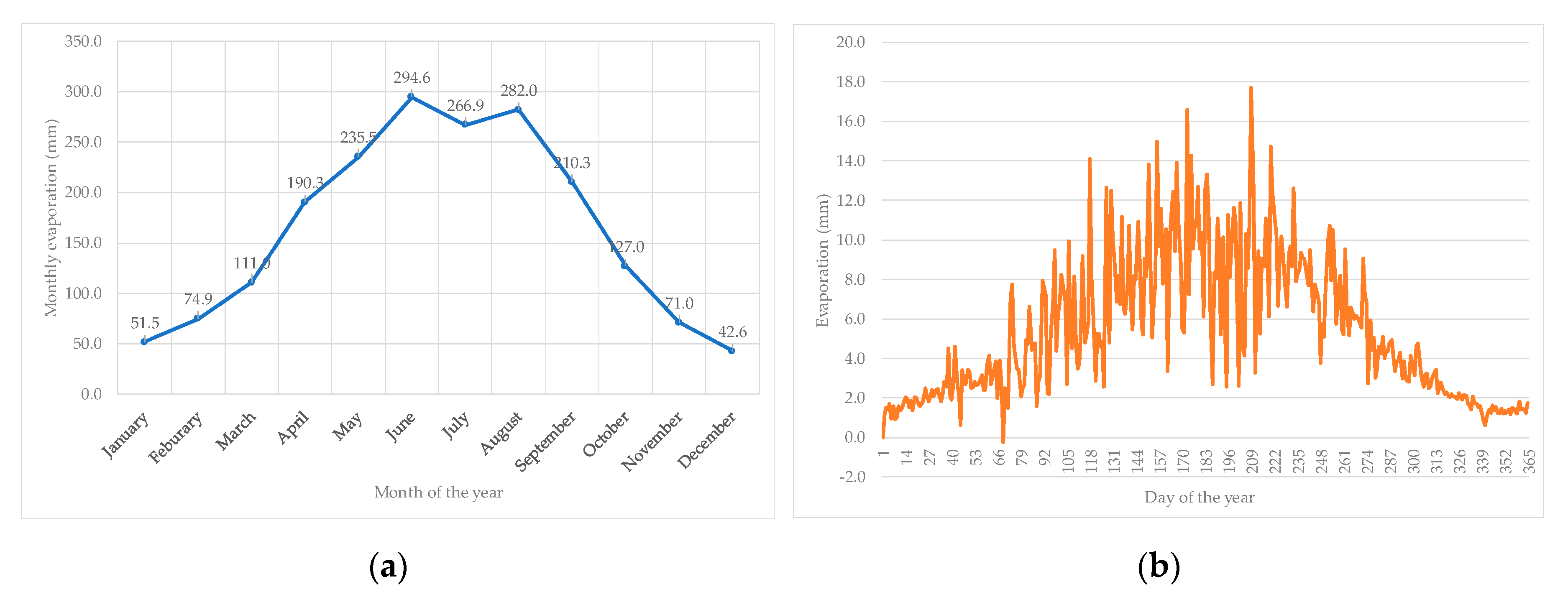
3.1. Water Evaporation

The results from the water evaporation model simulation at Lake Mead show an evaporation rate estimate of 1957 mm in 2018. This result is in agreement with the results of the study conducted by Moreo and Swancar [55] on Lake Mead during the period of March 2010 through February 2012 using the eddy covariance evaporation method. The study estimated the lake evaporation from March 2010 to February 2011, and from March 2011 to February 2012. According to the two authors, the evaporation rate for the first study period had a minimum value of 1958 mm and a maximum value of 2190 mm; while the minimum value was 1787 mm and the maximum value was 1975 mm for the second study period. The result obtained in this present study is located within the result interval of Moreo and Swancar’s study. Another early study by Westenburg et al. provided the evaporation data for Lake Mead from 1997 to 1999 [95]. The average evaporation rate for that period was 2281 mm.

Figure 4a shows the monthly results of the evaporation rates’ simulation using 2018 data. The evaporation rate is low in the winter and increases in summer. The evaporation rate at the peak of the summer, in June, is approximately five times more important than the lowest evaporation rate of the winter, in December. Figure 4b shows the daily evaporation estimates throughout the year.

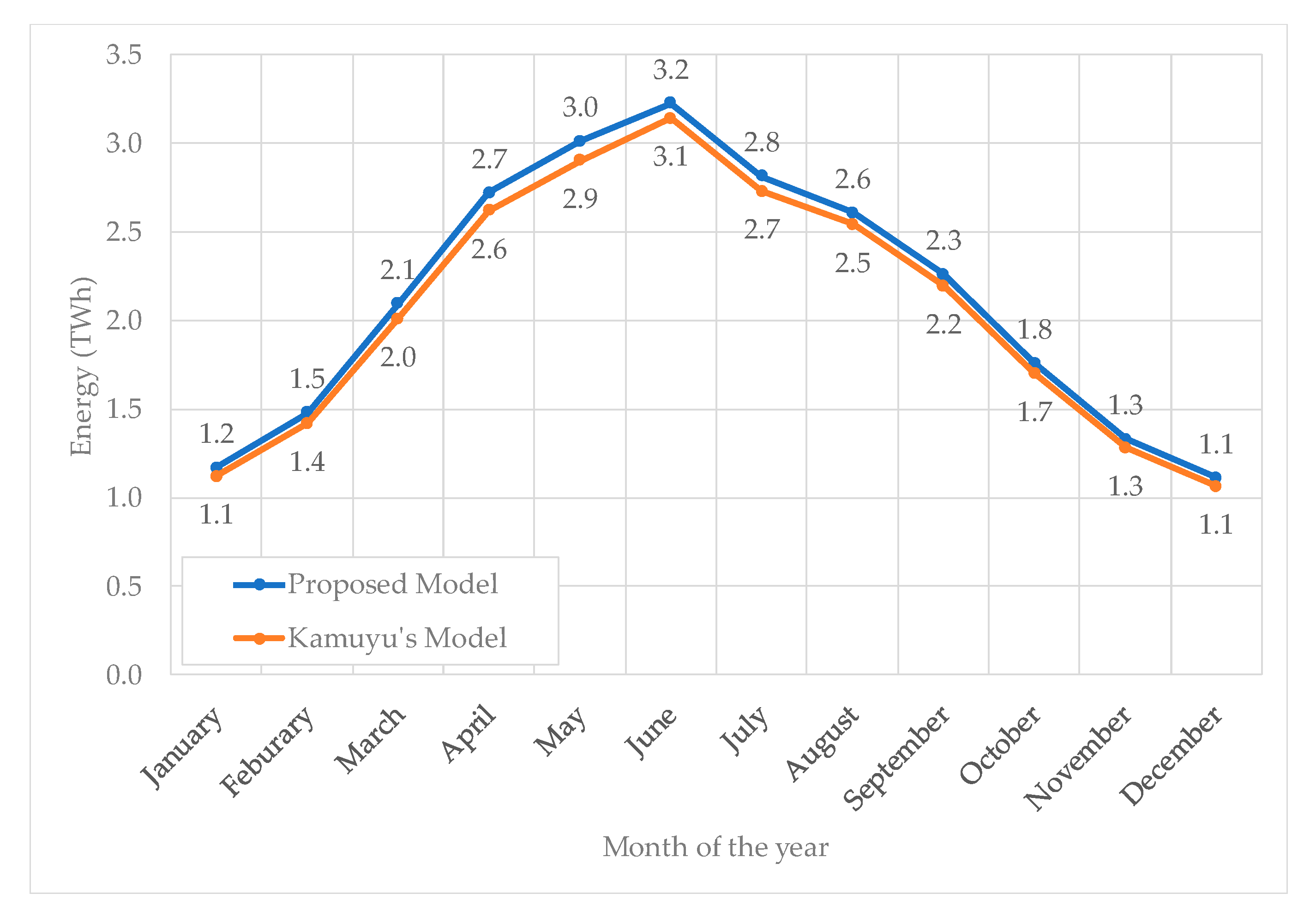
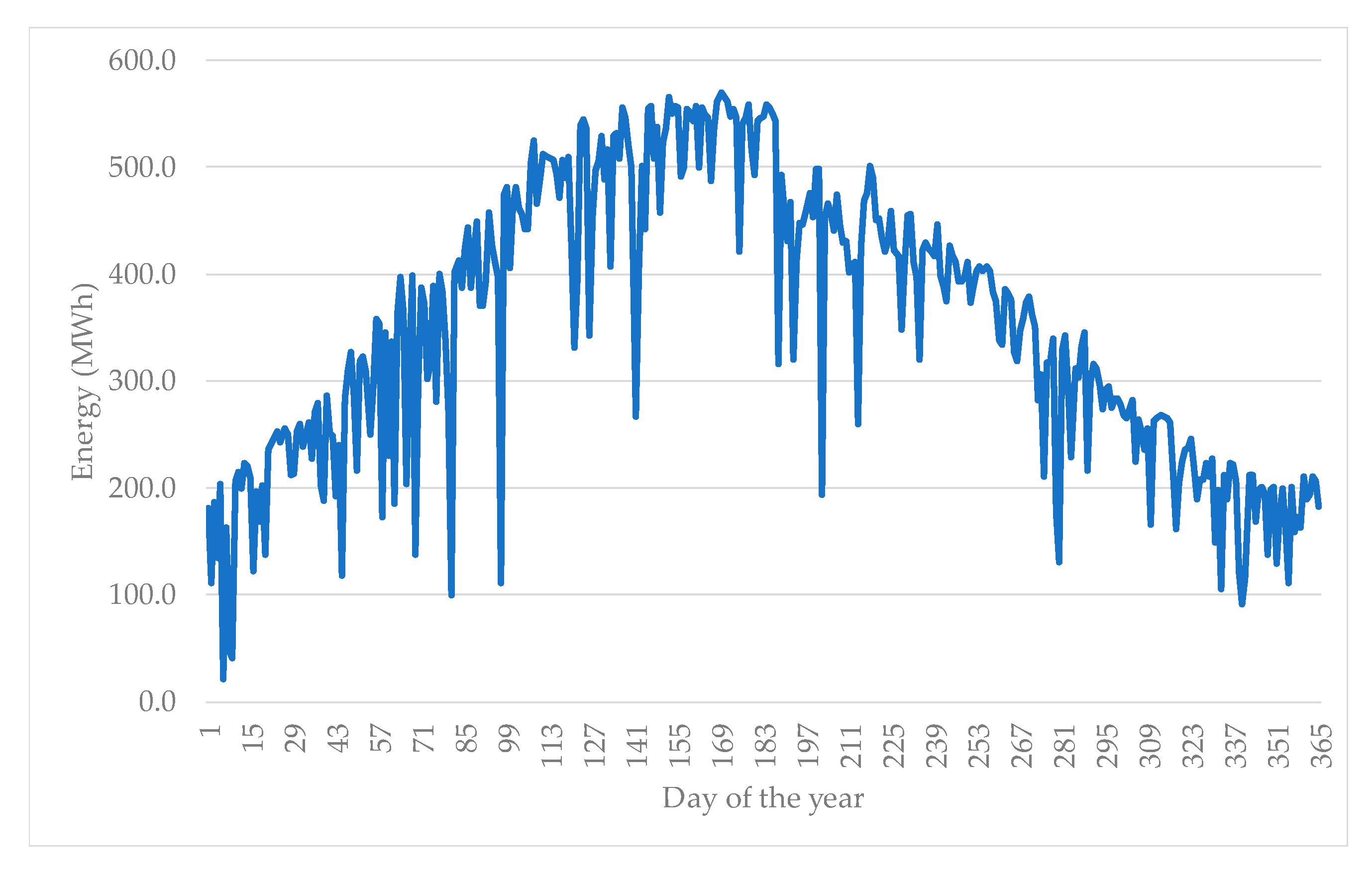
3.2. Energy Production

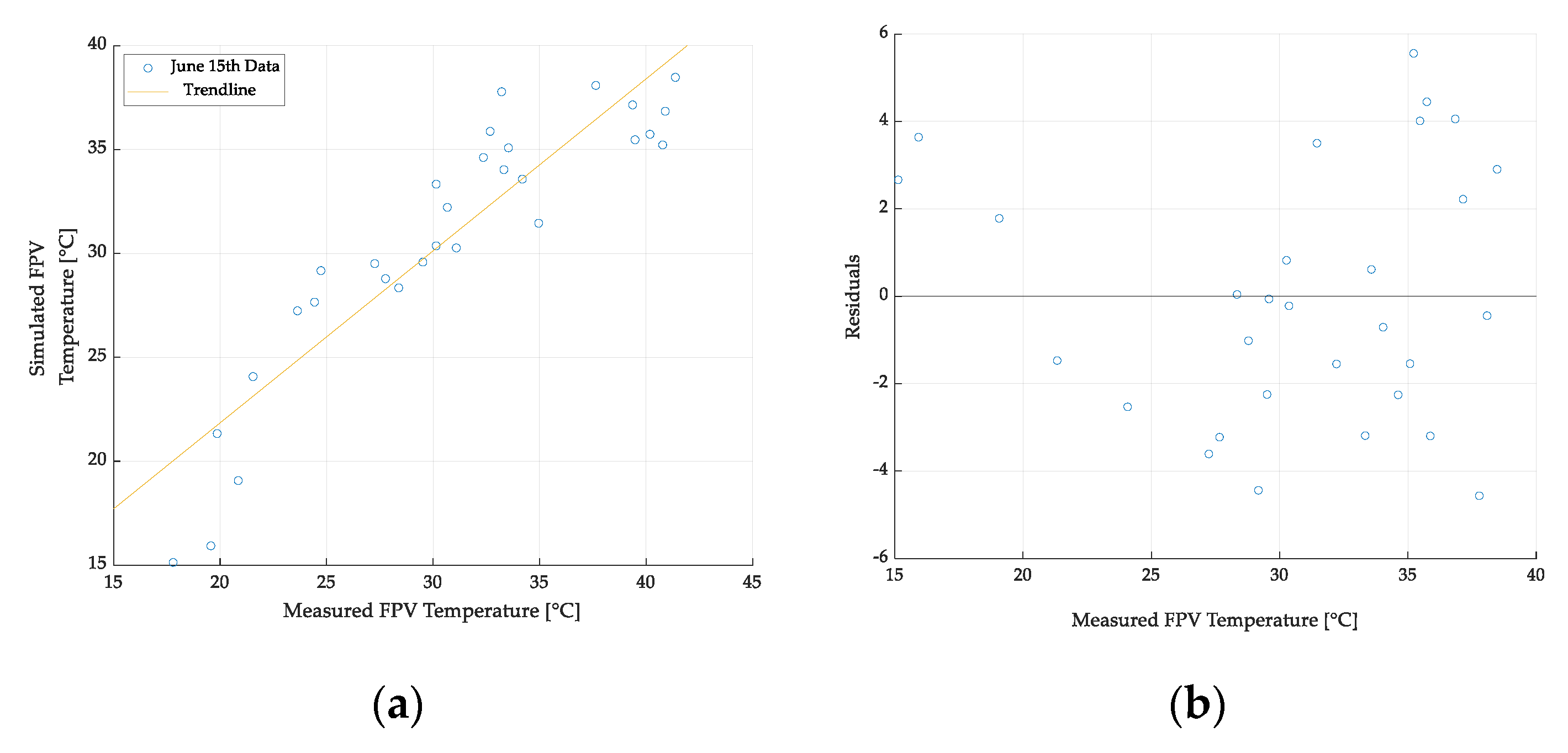
3.2.1. FPV Operating Temperature Model

The multilinear regression on the collected data yielded the coefficients ${\alpha }_0$, ${\alpha }_1$, ${\alpha }_2$, and ${\alpha }_3$, which describe the relationship between the FPV effective operating temperature (T_eo) and the independent variables: the water temperature (T_w), the air temperature (T_a), and the solar irradiance (I_S). The regression coefficients have been obtained with an R-squared value of 0.8276. Figure 5 shows the statistical results of the regression. The R-squared value combined with the random distribution of the residuals’ plot on Figure 5b show that there is a linear relationship between T_eo and the independent variables.

Equation (28) is proposed as a model that represents the effective operation temperature of FPV mounted on a foam-based support.

$$T_{eo}=-13.2554-0.0875\times T_w+1.2645\times T_a+0.0128\times I_S \left(°\mathrm{C}\right)$$

(28)

Figure 6 shows the simulated operating temperature using the proposed model, the operating temperature of a titled aluminum pontoon-based mount FPV model based on the original Kamuyu et al.’s model (for pontoon-based tilted FPV), and the measured operating temperature for June 15 2020. The simulated temperature is at times higher or lower than the measured temperature, but the overall trend of the two temperature profiles matches. The model proposed in this study is compared to the unadapted tilted FPV model and the current model (which is an adaptation of Kamuyu et al.’s model for foam-backed flat-surface FPV) and provides a better description of a foam-based FPV panel’s operating temperature. The proposed model in this study has a similar profile to Kamuyu’s model, and the proposed model provides a better description of the foam-based solar module’s behavior.

The temperature profile of a foam-based FPV panel installed on Lake Mead has been simulated using the proposed FPV operating temperature model and compared to a pontoon-based FPV as described by Kamuyu’s model in Figure 7.

The maximum temperature obtained with the model proposed in this study is 48.7 °C and the minimum temperature is −8.5 °C. On the other hand, the maximum temperature and the minimum temperature obtained if the FPV system was tilted are, respectively, 58.2 °C and −3.4 °C. Overall, the temperature model used here based on experimental data during the summer months predicts a lower temperature when the panels are in direct contact with the water surface.

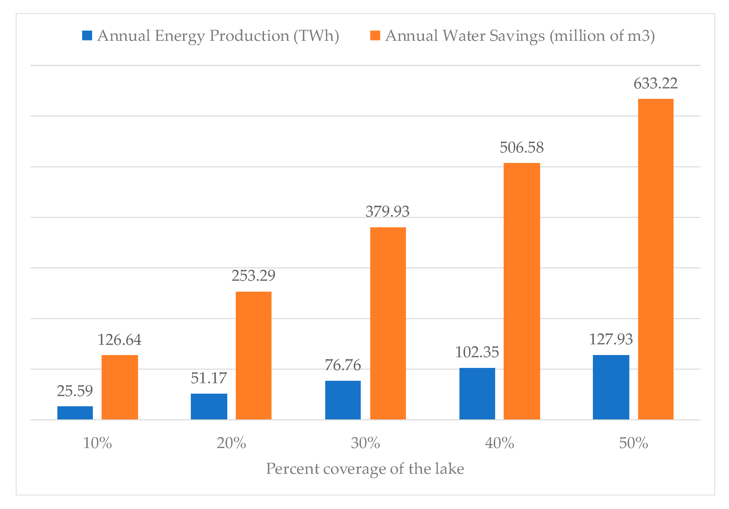
3.2.2. Energy Yield and Water Savings of an FPV System Installed on Lake Mead

The temperature profile is used to estimate the electrical efficiency of the solar panel, which is in turn used to simulate the energy yield of an FPV system installed on Lake Mead with historical weather data. The energy yield has been simulated by assuming a coverage of the lake surface between 10 and 50% in 10% increments. The results are shown in detail for the 10% coverage case and the total energy production is shown for the other cases.

Figure 8 shows the comparison between the monthly energy production obtained using the proposed model and the energy production of a tilted FPV for 10% coverage of the lake’s surface. As can be seen in Figure 8 and expected from Figure 7, the proposed model predicts a slightly higher energy production, about 3.5%, which is correlated with the lower operating temperature of the modules. The maximum energy per month production is 3.2 TWh and occurs in the month of June, while the minimum energy per month production is 1.1 TWh and occurs in December.

Figure 9 shows the result for the daily energy simulation when 10% of Lake Mead’s surface is covered with a foam-based solar FPV system. The maximum daily energy production is 570 MWh on 6 January while the minimum daily production is 21 MWh on 18 June.

Figure 10 shows the simulated annual energy production, and the water saving capabilities of a foam-based solar FPV system installed on the surface of Lake Mead as a function of coverage area from 10–50%. For a coverage of 10%, the annual production using collected temperature data is 25.59 TWh, corresponding to a saved water volume of 126.64 million m³. When the percentage coverage is increased, the energy production is increased linearly. For a coverage of 50% of the lake’s surface, it is possible to harvest 127.93 TWh of electrical energy and save 633.22 million of m³ of water using foam-based FPV panels.

Table 2. Estimation of the yearly cost of water saved and energy produced using water and energy cost range from Nevada for an FPV system covering 10–50% of Lake Mead’s surface.

Lake Surface Percent Coverage	Water Savings at $0.35/m3 (Millions of $)	Water Savings at $1.37/m3 (Millions of $)	Energy Revenues at 2¢/kWh (Billions of $)
10%	43.99	172.19	0.51
20%	87.98	344.37	1.02
30%	131.97	516.56	1.54
40%	175.96	688.75	2.05
50%	219.95	860.94	2.56

shows the annual water and energy savings estimates related to the water savings and energy production from the FPV. With houses with the least water consumption, the cost of the water saved is estimated to be USD 44 million when 10% of the lake surface is covered, and USD 220 million when 50% of the lake surface is covered. On the other hand, when the consumers’ water consumption is on the high side, these costs increase, amounting to USD 172 million when 10% of the lake is covered and USD 861 million when 50% is covered. Furthermore, the results for the energy production show that USD 0.5 billion of energy can be generated when 10% of the lake surface is covered. The value of the energy generated when 50% of the lake surface is covered is estimated as USD 2.6 billion.

The relative values of the water and energy provided by the foam-based FPV indicate that the electricity production from the FPV could be used to subsidize water conservation in arid and semi-arid areas. Thus, FPV could be a self-funded water conservation approach.

4. Discussion

The water evaporation calculation performed in this study predicts a significant water saving potential for foam-based FPV systems on Lake Mead. The evaporation calculation using historical data has shown an annual evaporation estimate of 1957.6 mm for the lake. The result of the calculation performed in this study is in agreement with previous evaporation studies on Lake Mead [55,95]. The simulation results show annual water savings ranging from 126.64 to 633.22 million m³ depending on the percentage of the lake surface covered by the FPV system. According to the United States Environmental Protection Agency (US EPA), each American uses, on average, 88 gallons of water per day, resulting in an annual water consumption of 32,120 gallons or 121.59 m³ per capita [96]. The amount of water saved using foam-based FPV on Lake Mead will therefore be enough to supply water to more than five million Americans in the case that 50% of the lake surface is covered. This would make a significant impact on the cities near Lake Mead. The value is more than the four million population of the second largest city in the country, Los Angeles [97] or the entire population of Nevada of 3.1 million [98]. When 10% of the lake is covered by FPV panels, the amount of water saved is enough to supply water to the populations of both Henderson (320,189) and Las Vegas (651,319) or Las Vegas and Reno (255,601) in Nevada [99]. According to an analysis performed by Barsugli et al., Lake Mead has a 50% percent chance of going dry between 2035 and 2047 if nothing is done to stop the current draw down and evaporation rate of the lake [100]. Other studies on the management of the lake have resulted in the same conclusion [101,102]. These studies have shown the need for new ways to mitigate lake evaporation not only on Lake Mead, but on other lakes in the world, especially those located in arid environments. Floating solar photovoltaic technology provides a solution to limit evaporation of water surfaces and provide electrical energy for the surrounding populations.

The energy production analysis has yielded an annual energy production ranging from 25.9 TWh to 127.93 TWh for a coverage of the lake of 10%, and 50%, respectively. The energy production profile is in accordance with a previous FPV study conducted by Kamuyu et al. [45], showing an improvement of 10% from a ground-mount system. This is confirmed by the study of Pierce et al., who determined that the energy production improvement of an FPV systems is 5–10% compared to a ground-mount system for mono and polycrystalline silicon [54]. This is due to the cooling effect of the water on the FPV modules. According to the United States Energy Information Agency (US EIA), the average American household electricity consumption is 10,649 kWh per year. This means that the energy production of an FPV system covering 10% of Lake Mead has the capacity to power more than two million American homes [103]. This is more than the electricity needed to power the homes in Las Vegas, Henderson and Reno combined. On the other hand, the total electricity consumption in the U.S. according to 2018 statistics is 4178 TWh. This implies that the electricity production from a solar FPV system covering 50% of Lake Mead can supply 3% of the total electricity consumed in the U.S. and can replace more than 11% of the coal-fired power plants operating in the country; thus, contributing in a significant way to the reduction in the national carbon dioxide emissions [104] and the concomitant air pollution-related mortality [105,106,107,108]. This study is in agreement with past work showing enormous potential for FPV on water bodies in the U.S. [109].

The results of this study show that there are several benefits to implementing a foam-based FPV solar plant. Foam-based FPV avoids the issues related to land use in ground-mounted solar PV [110] and since the floating device is made of low-cost material, the racking cost is lower than other raft racking FPV technologies [54]. In addition, FPV systems in general have the potential to form agrivoltaic type systems [111] by merging with aquaculture to form aquavoltaics [112,113]. The flexible foam-backed FPV approach used here even makes mobile FPV possible. The FPV approach demonstrated here is less expensive than conventional pontoon-based FPV and has a slightly higher energy output per W because of the modules’ close proximity to the water. FPV racking in general is less costly than conventional ground mounted PV. Thus, as PV is already often the least costly method for new electricity production, it provides a potentially profitable means of reducing water evaporation in the world’s dwindling bodies of fresh water. Overall, the results of this study appear extremely promising. Solar FPV is a fairly new technology that is growing at a tremendous rate, but for it to reach its full potential, future work is needed to explore policies that sustain the development of this technology while also minimizing negative externalities. To accomplish this, a full life cycle analysis (LCA) study is needed on this technology.

Future work is also needed to experimentally verify the results of this study in different locations throughout the world. In addition, future work is needed to investigate fouling (and means to prevent it) in different bodies of water. More data should also be collected to further refine the temperature model and improve the energy production accuracy of the results shown here. Foam-based technology used as a floating device needs to be investigated more in order to have a commercially viable mass-produced FPV foam racking. The work shown here and completed previously was accomplished using after-market alterations of flexible PV modules. It should be pointed out that economic calculations used here assumed a 25 year lifetime for the PV modules. Although they are rated for extreme environments, guaranteed to resist corrosion and waterproof, the flexible SunPower modules only carry a 5 year warranty rather than the industry standard 25–30 year warranty. Future work to test the long-term performance of such systems is needed to ensure the reliability and safety of a foam-backed FPV as described in this article. In addition, future technical work is needed to investigate the potential for making flexible modules rated for high voltages that would be more appropriate for utility scale systems such as described in this study. The cost of the FPV racking would be further reduced by integrating bulk purchased foam into the PV manufacturing process. In addition, closed loop, circular economy [114,115,116] and industrial symbiosis [117] could be applied to the FPV manufacturing process. This would be expected to further reduce the cost of the FPV as well but may also necessitate policy intervention to ensure end of life recycling [118]. The polyethylene foam used here could be fabricated from recycled plastic waste [119,120,121], thereby further improving the environmental balance sheet for foam-backed FPV. Future studies can potentially look into the long-term stability of foam in water by analyzing the effect of different qualities of water on this material. Another aspect of foam-based rack where future work is needed is the mooring technology used to secure the FPV. Finally, the environmental impacts of the floating solar systems on marine life have not been fully established [60] and will be an interesting subject for future studies.

5. Conclusions

This study introduced a new approach to FPV using a flexible crystalline silicon module backed with foam, which is less expensive than conventional pontoon-based FPV racking and land-based PV racking. The results show that the foam-backed FPV had a lower operating temperature than conventional pontoon-based fixed tilt out-of-water FPV and thus a higher energy output per unit power because of the modules’ close proximity to the water. Thus, because PV costs are now normally the least costly method of new electricity production, the hypothetical large-scale foam-based FPV provides a potentially profitable means of reducing water evaporation in the world’s at-risk bodies of fresh water.

The case study of Lake Mead found that if 10% of the lake was covered with foam-backed FPV, there would be more than enough solar electricity generated to power the homes in Las Vegas, Henderson and Reno combined and enough water savings for Las Vegas and Reno. At 50% lake coverage, the foam-backed FPV would provide over 127 TWh of clean solar electricity and 633.2 million m³ of water savings, which would provide enough electricity to retire 11% of the polluting coal-fired plants in the U.S. and water for over five million Americans, annually.

References

1. Arnell, N. Climate change and global water resources. Glob. Environ. Chang. 1999, 9, S31–S49. [Google Scholar] [CrossRef]
2. Kummu, M.; Ward, P.J.; de Moel, H.; Varis, O. Is physical water scarcity a new phenomenon? Global assessment of water shortage over the last two millennia. Environ. Res. Lett. 2010, 5, 034006. [Google Scholar] [CrossRef] [Green Version]
3. Coyle, E.D. (Ed.) Understanding the Global Energy Crisis; Purdue Studies in Public Policy; Purdue University Press: West Lafayette, IN, USA, 2014; ISBN 978-1-55753-661-7. [Google Scholar]
4. Brown, L.R. Full Planet, Empty Plates: The New Geopolitics of Food Scarcity, 1st ed.; W.W. Norton & Company: New York, NY, USA, 2012; ISBN 978-0-393-08891-5. [Google Scholar]
5. Baum, S.D.; Denkenberger, D.C.; Pearce, J. Alternative Foods as a Solution to Global Food Supply Catastrophes. Solutions 2016, 7, 31–35. [Google Scholar]
6. Rockström, J.; Falkenmark, M.; Karlberg, L.; Hoff, H.; Rost, S.; Gerten, D. Future water availability for global food production: The potential of green water for increasing resilience to global change: Water availability for food production. Water Resour. Res. 2009, 45. [Google Scholar] [CrossRef] [Green Version]
7. Misra, A.K. Climate change and challenges of water and food security. Int. J. Sustain. Built Environ. 2014, 3, 153–165. [Google Scholar] [CrossRef] [Green Version]
8. Cook, J.; Oreskes, N.; Doran, P.T.; Anderegg, W.R.L.; Verheggen, B.; Maibach, E.W.; Carlton, J.S.; Lewandowsky, S.; Skuce, A.G.; Green, S.A.; et al. Consensus on consensus: A synthesis of consensus estimates on human-caused global warming. Environ. Res. Lett. 2016, 11, 048002. [Google Scholar] [CrossRef]
9. Solomon, S.; Intergovernmental Panel on Climate Change (Eds.) Climate Change 2007: The Physical Science Basis: Contribution of Working Group I to the Fourth Assessment Report of the Intergovernmental Panel on Climate Change; Cambridge University Press: New York, NY, USA, 2007; ISBN 978-0-521-88009-1. [Google Scholar]
10. Kellogg, W.W.; Schware, R. Climate Change and Society: Consequences of Increasing Atmospheric Carbon Dioxide, 1st ed.; Routledge: New York, NY, USA, 2019; ISBN 978-0-429-04873-9. [Google Scholar]
11. Bates, B.; Kundzewicz, Z.W.; Wu, S.; Palutikof, J.P. (Eds.) Climate Change and Water. Technical Paper of the Intergovernmental Panel on Climate Change; IPCC Technical Paper 6; IPCC Secretariat: Geneva, Switzerland, 2008; ISBN 978-92-9169-123-4. [Google Scholar]
12. Baker, E.; Fowlie, M.; Lemoine, D.; Reynolds, S.S. The Economics of Solar Electricity. Annu. Rev. Resour. Econ. 2013, 5, 387–426. [Google Scholar] [CrossRef] [Green Version]
13. de Wit, M.; Stankiewicz, J. Changes in Surface Water Supply Across Africa with Predicted Climate Change. Science 2006, 311, 1917–1921. [Google Scholar] [CrossRef] [Green Version]
14. Edenhofer, O.; Pichs-Madruga, R.; Sokohana, Y.; Farahani, E.; Kadner, S.; Seyboth, K.; Adler, A.; Baum, I.; Brunner, S.; Eickemeier, P.; et al. (Eds.) IPCC Climate Change 2014: Mitigation of Climate Change: Working Group III Contribution to the Fifth Assessment Report of the Intergovernmental Panel on Climate Change; Cambridge University Press: New York, NY, USA, 2014; ISBN 978-1-107-05821-7. [Google Scholar]
15. Pearce, J.M. Photovoltaics—A path to sustainable futures. Futures 2002, 34, 663–674. [Google Scholar] [CrossRef]
16. Creutzig, F.; Agoston, P.; Goldschmidt, J.C.; Luderer, G.; Nemet, G.; Pietzcker, R.C. The underestimated potential of solar energy to mitigate climate change. Nat. Energy 2017, 2, 17140. [Google Scholar] [CrossRef]
17. Calvert, K.; Pearce, J.M.; Mabee, W.E. Toward renewable energy geo-information infrastructures: Applications of GIScience and remote sensing that build institutional capacity. Renew. Sustain. Energy Rev. 2013, 18, 416–429. [Google Scholar] [CrossRef] [Green Version]
18. SEIA Siting, Permitting & Land Use for Utility-Scale Solar. Available online: https://www.seia.org/initiatives/siting-permitting-land-use-utility-scale-solar (accessed on 13 November 2020).
19. Kenny, R.; Law, C.; Pearce, J.M. Towards real energy economics: Energy policy driven by life-cycle carbon emission. Energy Policy 2010, 38, 1969–1978. [Google Scholar] [CrossRef]
20. Groesbeck, J.G.; Pearce, J.M. Coal with Carbon Capture and Sequestration is not as Land Use Efficient as Solar Photovoltaic Technology for Climate Neutral Electricity Production. Sci. Rep. 2018, 8, 13476. [Google Scholar] [CrossRef] [PubMed]
21. FAO (Ed.) How does International Price Volatility Affect Domestic Economies and Food Security; The state of food insecurity in the world; FAO: Rome, Italy, 2011; ISBN 978-92-5-106927-1. [Google Scholar]
22. Yasmeena, S.; Das, G.T.R. A Review on New Era of Solar Power Systems: Floatovoltaic Systems or Floating Solar Power Plants. JIC 2015, 3, 1–8. [Google Scholar] [CrossRef]
23. Majid, Z.A.A.; Ruslan, M.H.; Sopian, K.; Othman, M.Y.; Azmi, M.S.M. Study on Performance of 80 Watt Floating Photovoltaic Panel. J. Mech. Eng. Sci. 2014, 7, 1150–1156. [Google Scholar] [CrossRef]
24. Trapani, K.; Millar, D.L. The thin film flexible floating PV (T3F-PV) array: The concept and development of the prototype. Renew. Energy 2014, 71, 43–50. [Google Scholar] [CrossRef]
25. do Sacramento, E.M.; Carvalho, P.C.; de Araújo, J.C.; Riffel, D.B.; da Cruz Corrêa, R.M.; Neto, J.S. Scenarios for use of floating photovoltaic plants in Brazilian reservoirs. Iet Renew. Power Gener. 2015, 9, 1019–1024. [Google Scholar] [CrossRef]
26. Trapani, K.; Santafé, M.R. A review of floating photovoltaic installations: 2007–2013. Prog. Photovolt. Res. Appl. 2015, 23, 524–532. [Google Scholar] [CrossRef] [Green Version]
27. Patil, S.S.; Wagh, M.M.; Shinde, N.N. A review on floating solar photovoltaic power plants. Int. J. Sci. Eng. Res. 2017, 8, 789–794. [Google Scholar]
28. Kumar, N.M.; Kanchikere, J.; Mallikarjun, P. Floatovoltaics: Towards improved energy efficiency, land and water management. Int. J. Civ. Eng. Technol. 2018, 9, 1089–1096. [Google Scholar]
29. Haugwitz, F. Floating Solar PV Gains Global Momentum. Available online: https://www.pv-magazine.com/2020/09/22/floating-solar-pv-gains-global-momentum/ (accessed on 3 October 2020).
30. Rosa-Clot, M.; Rosa-Clot, P.; Tina, G.M.; Scandura, P.F. Submerged photovoltaic solar panel: SP2. Renew. Energy 2010, 35, 1862–1865. [Google Scholar] [CrossRef]
31. Tina, G.M.; Rosa-Clot, M.; Rosa-Clot, P.; Scandura, P.F. Optical and thermal behavior of submerged photovoltaic solar panel: SP2. Energy 2012, 39, 17–26. [Google Scholar] [CrossRef]
32. Ferrer-Gisbert, C.; Ferrán-Gozálvez, J.J.; Redón-Santafé, M.; Ferrer-Gisbert, P.; Sánchez-Romero, F.J.; Torregrosa-Soler, J.B. A new photovoltaic floating cover system for water reservoirs. Renew Energy 2013, 60, 63–70. [Google Scholar] [CrossRef] [Green Version]
33. Abdulgafar, S.A.; Omar, O.S.; Yousif, K.M. Improving the efficiency of polycrystalline solar panel via water immersion method. IJIRSET 2014, 3, 96–101. [Google Scholar]
34. Mehrotra, S.; Rawat, P.; Debbarma, M.; Sudhakar, K. Performance of a solar panel with water immersion cooling technique. Int. J. Sci. Environ. Technol. 2014, 3, 1161–1172. [Google Scholar]
35. McKay, A. Floatovoltaics: Quantifying the Benefits of a Hydro-Solar Power Fusion; Pomona College: Claremont, CA, USA, 2013. [Google Scholar]
36. Santafé, M.R.; Gisbert, P.S.F.; Romero, F.J.S.; Soler, J.B.T.; Gozálvez, J.J.F.; Gisbert, C.M.F. Implementation of a photovoltaic floating cover for irrigation reservoirs. J. Clean. Prod. 2014, 66, 568–570. [Google Scholar] [CrossRef] [Green Version]
37. Sharma, P.; Muni, B.; Sen, D. Design parameters of 10 KW floating solar power plant. In Proceedings of the International Advanced Research Journal in Science, Engineering and Technology (IARJSET), National Conference on Renewable Energy and Environment (NCREE-2015), Ghaziabad, India, 1 May 2015; Volume 2. [Google Scholar]
38. Rosa-Clot, M.; Tina, G.M.; Nizetic, S. Floating photovoltaic plants and wastewater basins: An Australian project. Energy Procedia 2017, 134, 664–674. [Google Scholar] [CrossRef]
39. Liu, L.; Wang, Q.; Lin, H.; Li, H.; Sun, Q.; Wennersten, R. Power Generation Efficiency and Prospects of Floating Photovoltaic Systems. Energy Procedia 2017, 105, 1136–1142. [Google Scholar] [CrossRef]
40. Mittal, D.; Saxena, B.K.; Rao, K.V.S. Floating solar photovoltaic systems: An overview and their feasibility at Kota in Rajasthan. In Proceedings of the 2017 International Conference on Circuit, Power and Computing Technologies (ICCPCT), Kollam, India, 20–21 April 2017; IEEE: New York, NY, USA, 2017; pp. 1–7. [Google Scholar]
41. Mittal, D.; Saxena, B.K.; Rao, K.V.S. Potential of floating photovoltaic system for energy generation and reduction of water evaporation at four different lakes in Rajasthan. In Proceedings of the 2017 International Conference on Smart Technologies for Smart Nation (SmartTechCon), Bengaluru, India, 17–19 August 2017; pp. 238–243. [Google Scholar]
42. Abid, M.; Abid, Z.; Sagin, J.; Murtaza, R.; Sarbassov, D.; Shabbir, M. Prospects of floating photovoltaic technology and its implementation in Central and South Asian Countries. Int. J. Environ. Sci. Technol. 2019, 16, 1755–1762. [Google Scholar] [CrossRef]
43. Teixeira, L.E.; Caux, J.; Beluco, A.; Bertoldo, I.; Louzada, J.A.S.; Eifler, R.C. Feasibility Study of a Hydro PV Hybrid System Operating at a Dam for Water Supply in Southern Brazil. JPEE 2015, 3, 70–83. [Google Scholar] [CrossRef] [Green Version]
44. Vasco, G.; Silva, J.S.; Beluco, A. Feasibility Study of a PV Hydro Hybrid System, With Photovoltaic Panels on Floating Structures. Iop Conf. Ser. Mater. Sci. Eng. 2018, 366, 012011. [Google Scholar] [CrossRef]
45. Kamuyu, W.C.L.; Lim, J.; Won, C.; Ahn, H. Prediction Model of Photovoltaic Module Temperature for Power Performance of Floating PVs. Energies 2018, 11, 447. [Google Scholar] [CrossRef] [Green Version]
46. Ranjbaran, P.; Yousefi, H.; Gharehpetian, G.B.; Astaraei, F.R. A review on floating photovoltaic (FPV) power generation units. Renew. Sustain. Energy Rev. 2019, 110, 332–347. [Google Scholar] [CrossRef]
47. Lee, A.-K.; Shin, G.-W.; Hong, S.-T.; Choi, Y.-K. A study on development of ICT convergence technology for tracking-type floating photovoltaic systems. SGCE 2014, 3, 80–87. [Google Scholar] [CrossRef]
48. Song, J.; Choi, Y. Analysis of the Potential for Use of Floating Photovoltaic Systems on Mine Pit Lakes: Case Study at the Ssangyong Open-Pit Limestone Mine in Korea. Energies 2016, 9, 102. [Google Scholar] [CrossRef]
49. Choi, Y.K.; Choi, W.S.; Lee, J.H. Empirical Research on the Efficiency of Floating PV Systems. Sci. Adv. Mater. 2016, 8, 681–685. [Google Scholar] [CrossRef] [Green Version]
50. Stachiw, J.D. Performance of Photovoltaic Cells in Undersea Environment. J. Manuf. Sci. Eng. 1980, 102, 51–59. [Google Scholar] [CrossRef]
51. Rathod, M.K.; Banerjee, J. Thermal stability of phase change materials used in latent heat energy storage systems: A review. Renew. Sustain. Energy Rev. 2013, 18, 246–258. [Google Scholar] [CrossRef]
52. Ho, C.J.; Chou, W.-L.; Lai, C.-M. Thermal and electrical performance of a water-surface floating PV integrated with a water-saturated MEPCM layer. Energy Convers. Manag. 2015, 89, 862–872. [Google Scholar] [CrossRef]
53. Ho, C.J.; Chou, W.-L.; Lai, C.-M. Thermal and electrical performances of a water-surface floating PV integrated with double water-saturated MEPCM layers. Appl. Therm. Eng. 2016, 94, 122–132. [Google Scholar] [CrossRef]
54. Mayville, P.; Patil, N.V.; Pearce, J.M. Distributed Manufacturing of After Market Flexible Floating Photovoltaic Modules. J. Clean. Prod. 2020, in press. [Google Scholar] [CrossRef]
55. Moreo, M.T.; Swancar, A. Evaporation from Lake Mead, Nevada and Arizona, March 2010 through February 2012; Scientific Investigations Report; U.S. Geological Survey: Reston, VA, USA, 2013; p. 52.
56. NPS Overview of Lake Mead-Lake Mead National Recreation Area (U.S. National Park Service). Available online: https://www.nps.gov/lake/learn/nature/overview-of-lake-mead.htm (accessed on 29 June 2020).
57. Monteith, J.L. Evaporation and environment. Symp. Soc. Exp. Biol. 1965, 19, 205–234. [Google Scholar] [PubMed]
58. Allen, R.G.; FAO. Crop Evapotranspiration: Guidelines for Computing Crop Water Requirements; FAO Irrigation and Drainage Paper; Food and Agriculture Organization of the United Nations: Rome, Italy, 1998; ISBN 978-92-5-104219-9. [Google Scholar]
59. Hayibo, K.S.; Pearce, J.M. Calculations for Water Conservation Potential of Self-funded Foam-Based Flexible Surface-Mounted Floatovoltaics. OSF 2020. Available online: https://osf.io/twexy/ (accessed on 16 October 2020).
60. World Bank Group; ESMAP; SERIS. Where Sun Meets Water: Floating Solar Handbook for Practitioners; World Bank Group: Washington, DC, USA, 2019. [Google Scholar]
61. US Department of Commerce, N.O. and A.A. NDBC Station Page. Available online: http://www.ndbc.noaa.gov/station_page.php?station=nbba3 (accessed on 22 June 2020).
62. Weather Underground Las Vegas, NV Weather History | Weather Underground. Available online: https://www.wunderground.com/history/daily/us/nv/las-vegas/KLAS/date/2018-2-28 (accessed on 22 June 2020).
63. Solcast Solar Irradiance Data 2020. Available online: https://solcast.com (accessed on 19 September 2020).
64. NPS Storage Capacity of Lake Mead-Lake Mead National Recreation Area (U.S. National Park Service). Available online: https://www.nps.gov/lake/learn/nature/storage-capacity-of-lake-mead.htm (accessed on 22 June 2020).
65. US Department of Commerce, N.O. and A.A. NDBC Station History Page. Available online: http://www.ndbc.noaa.gov/station_history.php?station=nbba3 (accessed on 23 June 2020).
66. Hayibo, K.S. Soul-Ash/floating-pv: Lake Mead Data Cleaning Code; Zenodo, 2020; Available online: https://zenodo.org/record/3960777 (accessed on 26 July 2020).
67. Zotarelli, L.; Dukes, M.D.; Romero, C.C.; Migliaccio, K.W. Step by Step Calculation of the Penman-Monteith Evapotranspiration (FAO-56 Method); University of Florida: Gainesville, FL, USA, 2018. [Google Scholar]
68. Weiss, A.; Hays, C.J. Calculating daily mean air temperatures by different methods: Implications from a non-linear algorithm. Agric. For. Meteorol. 2005, 128, 57–65. [Google Scholar] [CrossRef]
69. Shi, T.-T.; Guan, D.-X.; Wu, J.-B.; Wang, A.-Z.; Jin, C.-J.; Han, S.-J. Comparison of methods for estimating evapotranspiration rate of dry forest canopy: Eddy covariance, Bowen ratio energy balance, and Penman-Monteith equation. J. Geophys. Res. Atmos. 2008, 113. [Google Scholar] [CrossRef]
70. Sunpower® SunPower Flexible Solar Panels | SPR-E-Flex-110. Available online: https://us.sunpower.com/sites/default/files/110w-flexible-panel-spec-sheet.pdf (accessed on 13 October 2020).
71. Foam Factory Foam Factory. Data Sheets | Foam Factory, Inc. Available online: https://www.foambymail.com/datasheets.html (accessed on 13 October 2020).
72. Domany, M.A.; Touchart, L.; Bartout, P.; Nedjai, R. The Evaporation From Ponds In The French Midwest. Lakes Reserv. Ponds 2013, 7, 75–88. [Google Scholar]
73. Abtew, W.; Melesse, A. Evaporation and Evapotranspiration; Springer: Dordrecht, The Netherlands, 2013; ISBN 978-94-007-4736-4. [Google Scholar]
74. Jensen, M.E.; Dotan, A.; Sanford, R. Penman-Monteith Estimates of Reservoir Evaporation. In Proceedings of the Impacts of Global Climate Change; American Society of Civil Engineers: Anchorage, AK, USA, 2005; pp. 1–24. [Google Scholar]
75. Finch, J.W.; Hall, R.L.; Great Britain; Environment Agency. Estimation of Open Water Evaporation: A Review of Methods; Environment Agency: Bristol, UK, 2005; ISBN 978-1-85705-604-4.
76. McJannet, D.L.; Webster, I.T.; Cook, F.J. An area-dependent wind function for estimating open water evaporation using land-based meteorological data. Environ. Model. Softw. 2012, 31, 76–83. [Google Scholar] [CrossRef]
77. Idso, S.B.; Jackson, R.D. Thermal radiation from the atmosphere. J. Geophys. Res. 1969, 74, 5397–5403. [Google Scholar] [CrossRef]
78. Mekonnen, M.M.; Hoekstra, A.Y. The blue water footprint of electricity from hydropower. Hydrol. Earth Syst. Sci. 2012, 16, 179–187. [Google Scholar] [CrossRef] [Green Version]
79. Jegede, O.O.; Ogolo, E.O.; Aregbesola, T.O. Estimating net radiation using routine meteorological data at a tropical location in Nigeria. Int. J. Sustain. Energy 2006, 25, 107–115. [Google Scholar] [CrossRef]
80. Niclòs, R.; Valor, E.; Caselles, V.; Coll, C.; Sánchez, J.M. In situ angular measurements of thermal infrared sea surface emissivity—Validation of models. Remote Sens. Environ. 2005, 94, 83–93. [Google Scholar] [CrossRef]
81. de Bruin, H.A.R. Temperature and energy balance of a water reservoir determined from standard weather data of a land station. J. Hydrol. 1982, 59, 261–274. [Google Scholar] [CrossRef]
82. Finch, J.W. A comparison between measured and modelled open water evaporation from a reservoir in south-east England. Hydrol. Process. 2001, 15, 2771–2778. [Google Scholar] [CrossRef]
83. McJannet, D. Estimating Open Water Evaporation for the Murray-Darling Basin; CSIRO: Water for a Healthy Country National Research Flagship: Canberra, Australia, 2008. [Google Scholar] [CrossRef]
84. Duffie, J.A.; Beckman, W.A. Chapter 23-Design of Photovoltaic Systems. In Solar Engineering of Thermal Processes; John, A.D., William, A.B., Eds.; John Wiley: Hoboken, NJ, USA, 2013; ISBN 978-0-470-87366-3. [Google Scholar]
85. Shaari, S.; Sopian, K.; Amin, N.; Kassim, M.N. The Temperature Dependence Coefficients of Amorphous Silicon and Crystalline Photovoltaic Modules Using Malaysian Field Test Investigation. Am. J. Appl. Sci. 2009, 6, 586–593. [Google Scholar] [CrossRef]
86. Kamkird, P.; Ketjoy, N.; Rakwichian, W.; Sukchai, S. Investigation on Temperature Coefficients of Three Types Photovoltaic Module Technologies under Thailand Operating Condition. Procedia Eng. 2012, 32, 376–383. [Google Scholar] [CrossRef] [Green Version]
87. MathWorks Multiple Linear Regression-MATLAB Regress. Available online: https://www.mathworks.com/help/stats/regress.html (accessed on 30 July 2020).
88. Maghami, M.R.; Hizam, H.; Gomes, C.; Radzi, M.A.; Rezadad, M.I.; Hajighorbani, S. Power loss due to soiling on solar panel: A review. Renew. Sustain. Energy Rev. 2016, 59, 1307–1316. [Google Scholar] [CrossRef] [Green Version]
89. Fouad, M.M.; Shihata, L.A.; Morgan, E.I. An integrated review of factors influencing the perfomance of photovoltaic panels. Renew. Sustain. Energy Rev. 2017, 80, 1499–1511. [Google Scholar] [CrossRef]
90. Jacobson, M.Z.; Jadhav, V. World estimates of PV optimal tilt angles and ratios of sunlight incident upon tilted and tracked PV panels relative to horizontal panels. Sol. Energy 2018, 169, 55–66. [Google Scholar] [CrossRef]
91. Taboada, M.E.; Cáceres, L.; Graber, T.A.; Galleguillos, H.R.; Cabeza, L.F.; Rojas, R. Solar water heating system and photovoltaic floating cover to reduce evaporation: Experimental results and modeling. Renew. Energy 2017, 105, 601–615. [Google Scholar] [CrossRef] [Green Version]
92. Las Vegas Valley Water District Water Rates. Available online: https://www.lvvwd.com/customer-service/pay-bill/water-rates.html (accessed on 16 October 2020).
93. Karambelkar, S. Hydropower Operations in the Colorado River Basin: Institutional Analysis of Opportunities and Constraints; Hydropower Foundation: Littleton, CP, USA, 2018; p. 91. [Google Scholar]
94. Trabish, H.K. Hoover Dam, the Drought, and a Looming Energy Crisis. Available online: https://www.utilitydive.com/news/hoover-dam-the-drought-and-a-looming-energy-crisis/281133/ (accessed on 13 November 2020).
95. Westenburg, C.L.; De Meo, G.A.; Tanko, D.J. Evaporation from Lake Mead, Arizona and Nevada, 1997–1999; U.S. Geological Survey: Reston, VA, USA, 2006; p. 34.
96. US EPA, O. Statistics and Facts. Available online: https://www.epa.gov/watersense/statistics-and-facts (accessed on 10 October 2020).
97. U.S. Census Bureau. U.S. Census Bureau QuickFacts: Los Angeles City, California. Available online: https://www.census.gov/quickfacts/losangelescitycalifornia (accessed on 10 October 2020).
98. U.S. Census Bureau. U.S. Census Bureau QuickFacts: Nevada. Available online: https://www.census.gov/quickfacts/NV (accessed on 13 October 2020).
99. U.S. Census Bureau. U.S. Census Bureau QuickFacts: Reno City, Nevada; Las Vegas City, Nevada; Henderson City, Nevada. Available online: https://www.census.gov/quickfacts/fact/table/renocitynevada,lasvegascitynevada,hendersoncitynevada/PST045219 (accessed on 13 October 2020).
100. Barsugli, J.J.; Nowak, K.; Rajagopalan, B.; Prairie, J.R.; Harding, B. Comment on “When will Lake Mead go dry?” by T. P. Barnett and D. W. Pierce: Commentary. Water Resour. Res. 2009, 45. [Google Scholar] [CrossRef] [Green Version]
101. Rajagopalan, B.; Nowak, K.; Prairie, J.; Hoerling, M.; Harding, B.; Barsugli, J.; Ray, A.; Udall, B. Water supply risk on the Colorado River: Can management mitigate? Water Resour. Res. 2009, 45. [Google Scholar] [CrossRef]
102. Barnett, T.P.; Pierce, D.W. When will Lake Mead go dry? Water Resour. Res. 2008, 44. [Google Scholar] [CrossRef] [Green Version]
103. U.S. EIA. Frequently Asked Questions (FAQs)-U.S. Energy Information Administration (EIA). Available online: https://www.eia.gov/tools/faqs/faq.php (accessed on 10 October 2020).
104. U.S. EIA. Electric Power Annual 2018; U.S. Energy Information Administration: Washington, DC, USA, 2019; p. 239.
105. Prehoda, E.W.; Pearce, J.M. Potential lives saved by replacing coal with solar photovoltaic electricity production in the U.S. Renew. Sustain. Energy Rev. 2017, 80, 710–715. [Google Scholar] [CrossRef] [Green Version]
106. Burney, J.A. The downstream air pollution impacts of the transition from coal to natural gas in the United States. Nat. Sustain. 2020, 3, 152–160. [Google Scholar] [CrossRef]
107. Thurston, G.D.; Burnett, R.T.; Turner, M.C.; Shi, Y.; Krewski, D.; Lall, R.; Ito, K.; Jerrett, M.; Gapstur, S.M.; Diver, W.R.; et al. Ischemic Heart Disease Mortality and Long-Term Exposure to Source-Related Components of U.S. Fine Particle Air Pollution. Environ. Health Perspect. 2016, 124, 785–794. [Google Scholar] [CrossRef] [Green Version]
108. Krewski, D.; Jerrett, M.; Burnett, R.T.; Ma, R.; Hughes, E.; Shi, Y.; Turner, M.C.; Pope, C.A., III; Thurston, G.; Calle, E.E.; et al. Extended Follow-Up and Spatial Analysis of the American Cancer Society Study Linking Particulate Air Pollution and Mortality; Health Effects Institute: Boston, MA, USA, 2009; p. 154. [Google Scholar]
109. Spencer, R.S.; Macknick, J.; Aznar, A.; Warren, A.; Reese, M.O. Floating Photovoltaic Systems: Assessing the Technical Potential of Photovoltaic Systems on Man-Made Water Bodies in the Continental United States. Environ. Sci. Technol. 2019, 53, 1680–1689. [Google Scholar] [CrossRef]
110. Gorjian, S.; Sharon, H.; Ebadi, H.; Kant, K.; Scavo, F.B.; Tina, G.M. Recent technical advancements, economics and environmental impacts of floating photovoltaic solar energy conversion systems. J. Clean. Prod. 2021, 278, 124285. [Google Scholar] [CrossRef]
111. Dinesh, H.; Pearce, J.M. The potential of agrivoltaic systems. Renew. Sustain. Energy Rev. 2016, 54, 299–308. [Google Scholar] [CrossRef] [Green Version]
112. Pringle, A.M.; Handler, R.M.; Pearce, J.M. Aquavoltaics: Synergies for dual use of water area for solar photovoltaic electricity generation and aquaculture. Renew. Sustain. Energy Rev. 2017, 80, 572–584. [Google Scholar] [CrossRef] [Green Version]
113. Moustafa, K. Toward Future Photovoltaic-Based Agriculture in Sea. Trends Biotechnol. 2016, 34, 257–259. [Google Scholar] [CrossRef] [Green Version]
114. Sica, D.; Malandrino, O.; Supino, S.; Testa, M.; Lucchetti, M.C. Management of end-of-life photovoltaic panels as a step towards a circular economy. Renew. Sustain. Energy Rev. 2018, 82, 2934–2945. [Google Scholar] [CrossRef]
115. Farrell, C.C.; Osman, A.I.; Doherty, R.; Saad, M.; Zhang, X.; Murphy, A.; Harrison, J.; Vennard, A.S.M.; Kumaravel, V.; Al-Muhtaseb, A.H.; et al. Technical challenges and opportunities in realising a circular economy for waste photovoltaic modules. Renew. Sustain. Energy Rev. 2020, 128, 109911. [Google Scholar] [CrossRef]
116. Lisperguer, R.C.; Cerón, E.M.; de la Casa Higueras, J.; Martín, R.D. Environmental Impact Assessment of crystalline solar photovoltaic panels’ End-of-Life phase: Open and Closed-Loop Material Flow scenarios. Sustain. Prod. Consum. 2020, 23, 157–173. [Google Scholar] [CrossRef]
117. Pearce, J.M. Industrial symbiosis of very large-scale photovoltaic manufacturing. Renew. Energy 2008, 33, 1101–1108. [Google Scholar] [CrossRef] [Green Version]
118. McDonald, N.C.; Pearce, J.M. Producer responsibility and recycling solar photovoltaic modules. Energy Policy 2010, 38, 7041–7047. [Google Scholar] [CrossRef] [Green Version]
119. Kabamba, E.T.; Rodrigue, D. The effect of recycling on LDPE foamability: Elongational rheology. Polym. Eng. Sci. 2008, 48, 11–18. [Google Scholar] [CrossRef]
120. Bedell, M.; Brown, M.; Kiziltas, A.; Mielewski, D.; Mukerjee, S.; Tabor, R. A case for closed-loop recycling of post-consumer PET for automotive foams. Waste Manag. 2018, 71, 97–108. [Google Scholar] [CrossRef]
121. Al-Sabagh, A.M.; Yehia, F.Z.; Eshaq, G.H.; Rabie, A.M.; ElMetwally, A.E. Greener routes for recycling of polyethylene terephthalate. Egypt. J. Pet. 2016, 25, 53–64. [Google Scholar] [CrossRef] [Green Version]
Figure 1. Cut away view showing adhesive underneath foam attached to c-Si-based flexible photovoltaic (PV) module: (a) top view and (b) orthogonal view.
Energies 13 06285 g001
Figure 2. Closeup of floating photovoltaic/floatovoltaic (FPV) corner after deployment, showing water coverage from a modest wave (top left).
Energies 13 06285 g002
Figure 3. Wiring diagram for NanoDAQ monitoring board.
Energies 13 06285 g003
Figure 4. Water evaporation simulation results for Lake Mead: (a) simulated evaporation values (mm) for each month of the year 2018; (b) simulated evaporation values (mm) for each day of the year 2018.
Energies 13 06285 g004
Figure 5. Multilinear regression results of the FPV panels’ effective operating temperature (Teo): (a) simulated FPV temperature plotted against the measured temperature for 15 June 2020; (b) residuals’ distribution plotted against the simulated FPV temperature for 15 June 2020.
Energies 13 06285 g005
Figure 6. Measured FPV operating temperature compared to simulated FPV operating temperature for 15 June 2020.
Energies 13 06285 g006
Figure 7. Operation temperature of an FPV installed on the surface of Lake Mead. (+) Operating temperature using the proposed model in this study for foam-based FPV. (o) Operating temperature using a ponton-based tilted FPV described by Kamuyu’s model.
Energies 13 06285 g007
Figure 8. Monthly energy yield of a simulated foam-based FPV system installed on 10% of Lake Mead’s surface using historical data from 2018. Comparison between the proposed model (c-Si flexible foam-backed FPV) and a tilted FPV based on Kamuyu’s model (c-Si aluminum mount FPV).
Energies 13 06285 g008
Figure 9. Daily energy production results using the temperature model proposed in this study for 10% coverage of Lake Mead’s surface.
Energies 13 06285 g009
Figure 10. Simulated annual energy production (TWh) and water saving capability (millions of m3) of a foam-based solar FPV system installed on Lake Mead’s surface using historical temperature data and the proposed model depending on the percentage coverage of the lake’s surface.
Energies 13 06285 g010