Time-Scale Economic Dispatch of Electricity-Heat Integrated System Based on Users’ Thermal Comfort

Abstract

The electricity-heat integrated system can realize the cascade utilization of energy and the coordination and complementarity between multiple energy sources. In this paper, considering the thermal comfort of users, taking into account the difference in dynamic characteristics of electric and heating networks and the response of users’ demands, a dispatch model is constructed. In this model, taking into account the difference in the time scale of electric and thermal dispatching, optimization of the system can be improved by properly extending the thermal balance cycle of the combined heat and power (CHP) unit. Based on the time-of-use electricity prices and heat prices to obtain the optimal energy purchase cost, a user demand response strategy is adopted. Therefore, a minimum economic cost on the energy supply side and a minimum energy purchase cost on the demand side are considered as a bilevel optimization strategy for the operation of the system. Finally, using an IEEE 30 nodes power network and a 31 nodes heating network to form an electricity-heat integrated system, the simulation results show that the optimal thermal balance cycle can maximize the economic benefits on the premise of meeting the users’ thermal comfort and the demand response can effectively realize the wind curtailment and improve the system economy.

1. Introduction

In energy demand, heat and electric energy are not only the basic needs of human production and life, but also the main energy forms of the integrated energy system. The interaction between power and thermal systems will play a significant role in efficiently promoting the economic transition to a low-carbon energy system with a high permeability of renewable energy. Electricity-heat integrated systems have become an inevitable trend to achieve the close integration of energy networks and improve the overall energy efficiency of the system [1,2,3,4].

At present, a lot of studies have been carried out to research the economic dispatch of electricity-heat integrated system [5,6,7]. Part of the literature decouples the constraints of combined heat and power (CHP) unit’s “using heat to determine electricity” by adding electricity-to-heat equipment and heat storage devices [8,9] or utilizing the heat storage capacity of the district heating network [10], thus improving the flexibility of the electricity-heat integrated system. In [11], the air source heat pump is proposed as an alternative to the electrification of European heating. A specific heat pump model is proposed and open data from building, climate, and economic sources are used for analysis. This kind of electric heating equipment can effectively reduce carbon emissions. The authors in [12] proposed a multi-time scale optimization method for the CHP microgrid containing renewable energy, and the operational optimization of the hybrid microgrid was completed through the “hour”, “minute” and “second” time scales. The authors in [3] described a mixed integer linear programming model for determining the optimal capacity and operation of seven combined cooling, heating and power systems in the heating and cooling network of a residential district (Shahid Beheshti Town) located in the east of Tehran. The economic and environmental results obtained from the scenarios revealed savings in costs and a reduction in CO₂ emissions in the optimal cogeneration system compared with using boilers to produce heat and buying electricity from the grid.

The wind power accommodation problem brings more challenges to the research of electricity-heat integrated systems. Most scholars have done a lot of research into improving the flexibility of CHP units, and improving the flexible peak-shaving capacity of electricity-heat integrated systems, which are the important means to solve the shortage of wind power accommodation [13]. In [14], a multi-level, multi-time-scale method was proposed to use a single demand-side resource to provide multiple system services at the same time, so as to alleviate the problem that insufficient flexibility would lead to the reduction of high-level renewable energy. Based on the time-of-use electricity price, a new energy optimal dispatching model considering the users’ comfort and power consumption economy of microgrid was proposed in [15]. In [16], in order to make full use of renewable energy and dispatch demand side resources more hierarchically, a bilevel optimal dispatch model of the microgrid considering customer satisfaction was proposed, and the resulting net loads could be treated as a link between the upper and lower layer dispatch.

In this paper, considering the improvement of the living standards of users, the heating system needs to adjust the heating quantity according to the change of ambient temperature, and makes the corresponding regulation and control according to the user’s somatosensory temperature. Buildings and district heating networks were used in [17] to realize energy storage to compensate for the reduced heat output of the district heating system. The obtained results were presented for the reference district heating system in Poland. Estimated consumption of heat from centralized sources, individual thermal generators, and heating stoves by the population of Russia is obtained in [18]. Segments of households are distinguished according to the type of thermal amenities and described, and the thermal comfort situation is analyzed. This kind of heating system, which takes the users’ comfort as the control target, puts forward higher requirements for the operation and regulation level of the heat supply network. In addition, due to the thermal inertia of thermal energy, there is a large delay in the transmission and consumption links, so the mode of total heat supply balance in a certain period of time which is the time scale of heat balance can be selected to achieve system economic optimization [19]. The size of the thermal balance time scale has a great impact on users’ comfort. Therefore, it is a key problem to select the optimal thermal balance dispatch time scale to achieve the balance between users’ comfort and the system operation economy. The contributions of this paper are organized as follows:

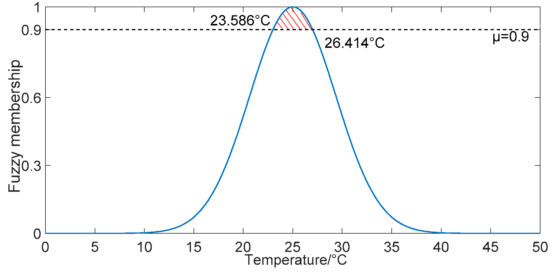
• Based on the outdoor temperature and the user’s thermal comfort, the fuzzy membership function can be used as the user’s thermal comfort index, which can scientifically reflect the relationship between heating power and users’ comfort reasonably, and put forward the concept of the heat demand envelope belt.
• Considering the users’ comfort index and the characteristics of the real-time power balance and total heat energy balance in the dispatch time scale, the thermal balance dispatch cycle model is established to find the balance point between user comfort and system economy. The thermal inertia of the heating network is used to fully excavate the system operation economy and improve the unit operation flexibility.
• Exploiting the available potential of user-side resources, a time-scale economic dispatch model of electricity-heat integrated systems considering thermal comfort is established. According to the relationship between time-sharing electricity price and thermal price, users can take a demand response (DR) action to obtain the optimal energy purchase cost.
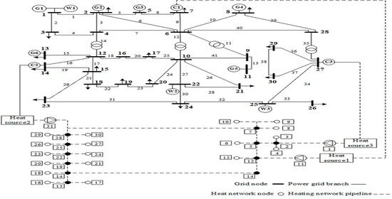
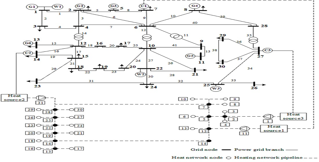
• Taking a typical winter day in a certain area of Liaoning Province of China as an example, considering the specific power network structure, the simulation results are more practical. The simulation results show that the optimization model can determine the optimal heat regulation time of the system, which meets the requirements of user comfort, improve the flexibility of the system, improve the system operation economy, and effectively improve the wind power absorption capacity.

2. Thermal Demand Modeling Method Considering Users’ Thermal Comfort

2.1. Indoor Temperature Model

At present, there are two common types of civil heating systems, which are hot water–air radiator convection heating systems or low temperature hot water floor radiant heating system. In this paper, a hot water air radiator convective heating system is adopted.

The inner surface of the heating radiator is hot water, and the outer surface side is indoor air. The radiator increases the indoor temperature by heating the indoor air. The heat dissipation power of the radiator $Q_{ra,t}$ can be described below:

$$Q_{ra,t}=c_w{m}_j(T_{in}-T_{out})$$

(1)

where $c_w$ is the specific heat capacity of water; $m_j$ is the mass flow of hot water in the water supply pipe connected to user j; $T_{in}$ and $T_{out}$ represent the inlet and outlet temperature of hot water, respectively.

Considering the temperature loss of the hot water pipe, the temperature of the inlet pipe and the outlet pipe of the house satisfy the following formula:

$$T_{in}=(T_{\mathrm{s}}-T_{\mathrm{r}})e^{-h{l}_s/c{m}^{\prime }}+T_a$$

(2)

$$T_{out}=(T_r-T_a)e^{h{l}_s/c{m}^{\prime }}+T_a$$

(3)

where h is the heat transfer coefficient; $l_{\mathrm{s}}$ is the length of the pipe; $m^{\prime }$ is the superior hot water mass flow connected to the user; $T_s$, $T_r$ and $T_a$ refer to the water supply temperature, return water temperature and outdoor temperature of the heat pipe in the heating network, respectively.

Thus the indoor temperature calculation formula is given as follows:

$$T_{n,t+1}=\{\begin{array}{ll}(T_{a,t}+Q_{ra,t}/\delta )(1-e^{-\Delta t/T_c})+T_{n,t}{e}^{-\Delta t/T_c}& U_{ra}=1\\ T_{a,t}(1-e^{-\Delta t/T_c})+T_{n,t}{e}^{-\Delta t/T_c}& U_{ra}=0\end{array}$$

(4)

where $T_{n,t+1}$ is the indoor temperature at time t + 1; $\delta$ is the air heat transfer coefficient; $\Delta t$ is the unit dispatch time; $T_c$ is the heat dispatch cycle of the electricity-heat integrated system; $U_{ra,t}$ represents the on–off state of the radiator during the t period; $U_{ra,t}=0$ and $U_{ra,t}=1$ represent the shutdown state and open state, respectively.

2.2. Users’ Thermal Comfort Index

While the electricity-heat integrated system improves the operating economy, it also needs to ensure users’ thermal comfort requirements. In order to simplify the analysis, this paper only uses temperature as a measure of the comfort level of people’s thermal perception. Therefore, we define a fuzzy membership function based on thermal comfort [20]:

$$\mu (T_n)=e^{-{(\frac{T_n-a}{b})}^2}b>0$$

(5)

where a and b are set values; $\mu$ is a fuzzy membership value based on user thermal comfort.

According to reference [21], the desired indoor temperature is influenced by the preference of the user, the local climate (temperature/humidity), the physical characteristics of the room (insulation, heat gain), etc. For example, the suitable indoor temperature ranges for people’s daily life is from 22 to 26 °C. This shows that people’s comfortable temperature in daily life tends to be in a fuzzy range. In order to reflect the user’s temperature preference more truly, we propose the fuzzy membership function. In this paper, we set a = 25 °C, b = 6.1616 and $\mu$ is set to be greater than 0.9; that is, when the indoor temperature is within the temperature range of 23.586 to 26.414 °C, the human body is at a more comfortable temperature. We can also adjust the values of a, b, and $\mu$ according to the different comfort requirements of different users. Therefore, the following research in this paper also makes the temperature maintain a range through the ambiguity of the user’s perception of temperature, and the thermal network does not need a real-time balance, so that the total heat demand can be adjusted within a certain range, which is more convenient to adjust the output of the thermal power unit to obtain a higher economy. The fuzzy membership function based on user thermal comfort is shown in Figure 1.

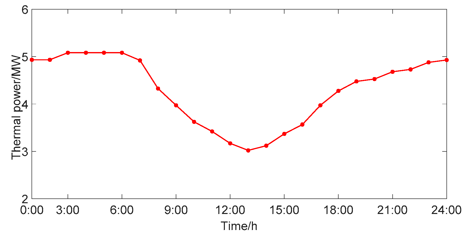
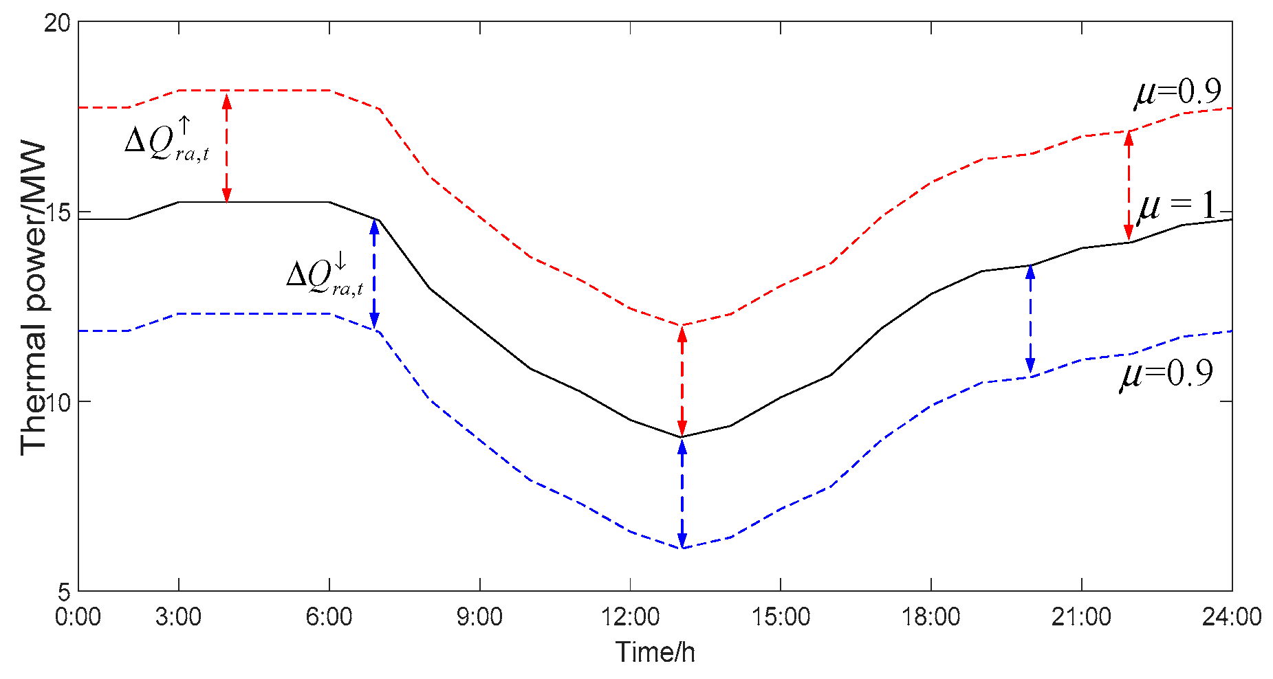
2.3. Thermal Demand Envelope Based on Users’ Thermal Comfort

The main heat dissipation device in the user room is a radiator, and the power of the radiator must meet the following constraints.

$$Q_{ra,t}=K_s{F}_s{N}_s(\frac{T_{in}+T_{out}}{2}-T_n)$$

(6)

where $K_s$ is the heat transfer coefficient of the radiator; $F_s$ is the heat dissipation area of the radiator; $N_s$ is the correction coefficient of the number of assembled pieces, connection forms and installation forms of the radiator.

Based on the user’s thermal comfort, the upper and lower limits of radiator output are given as follows:

$$\underset{\_}{Q_{ra,t}}\le Q_{ra,t}\le \overline{Q_{ra,t}}$$

(7)

$$\underset{\_}{Q_{ra,t}}=\frac{K_s{F}_s{N}_s}{1+\frac{K_s{F}_s{N}_s}{2c_w{m}_j}}\{(T_s-T_a)e^{-h{l}_s/c{m}^{\prime }}+T_a-\overline{T_n^{\underset{\_}{\mu }}}\}$$

(8)

$$\overline{Q_{ra,t}}=\frac{K_s{F}_s{N}_s}{1+\frac{K_s{F}_s{N}_s}{2c_w{m}_j}}\{(T_s-T_a)e^{-h{l}_s/c{m}^{\prime }}+T_a-\underset{\_}{T_n^{\underset{\_}{\mu }}}\}$$

(9)

where $\underset{\_}{\mu }$ is the user’s minimum thermal comfort standard and the corresponding upper and lower temperature is $\overline{T_n^{{\mu }_j}}$ and $\underset{\_}{T_n^{{\mu }_j}}$, so the upper and lower limits of the power of the user’s radiator are $\overline{Q_{ra,t}}$ and $\underset{\_}{Q_{ra,t}}$. ${\mu }_j$ is the comfort degree set for user j, and the indoor temperature of the user at time t must meet the comfort condition ${\mu }_j\le {\mu }_t\le 1$.

Adjustable range of user’s heat demand at each moment is expressed as follows:

$$\Delta Q_{ra,t}^{\uparrow }=c_w{m}_j(\overline{T_n^{{\mu }_j}}-T_n)$$

(10)

$$\Delta Q_{ra,t}^{\downarrow }=c_w{m}_j(T_n-\underset{\_}{T_n^{{\mu }_j}})$$

(11)

where $\Delta Q_{ra,t}^{\uparrow }$ and $\Delta Q_{ra,t}^{\downarrow }$ are the powers that can be increased and reduced by the user radiator at time t, that is, the adjustable range of thermal power to meet the user’s thermal comfort demand.

3. Time-Scale Dispatch Model of Electricity-Heat Integrated System

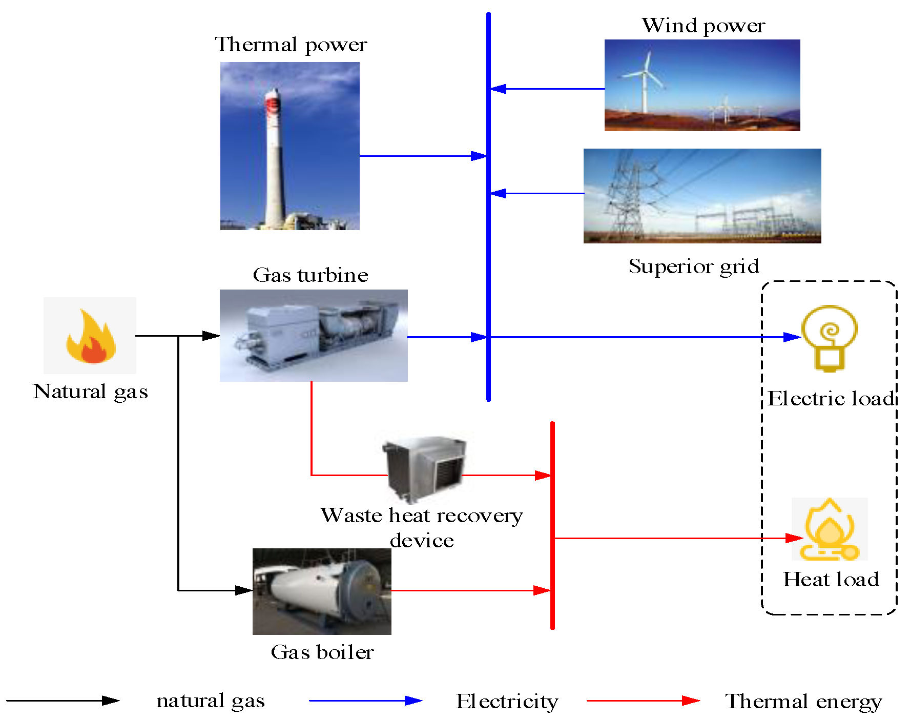
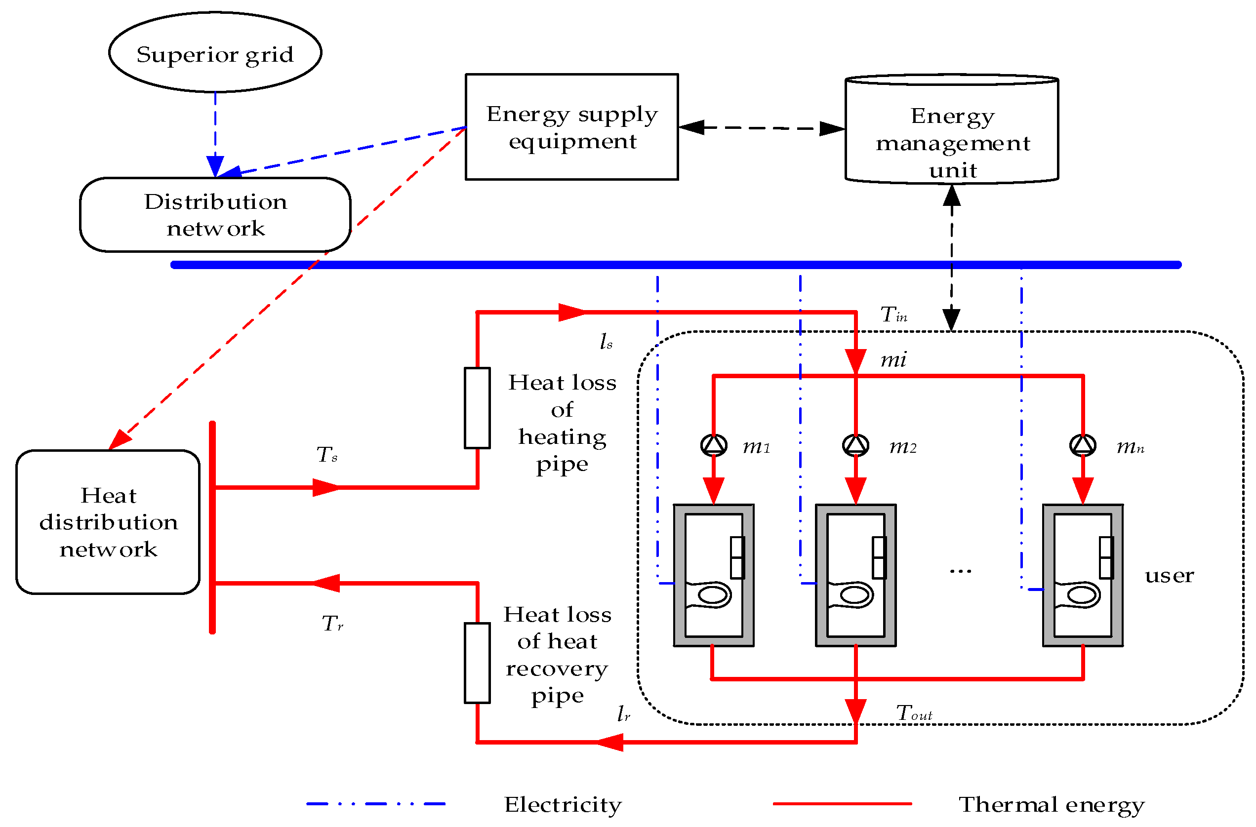
3.1. Electricity-Heat Integrated System Structure

The power supply network, heating network, heat storage system, control system coordinating the temperature balance of the supply and demand side, and the electric boiler equipment as a coupling link constitute the electricity-heat integrated system. The architecture is shown in Figure 2.

It can be seen from Figure 2 that the power grid, wind turbine, and gas turbine jointly supply power. The gas turbine and gas-fired boiler both use natural gas as fuel cooperating with each other to transmit the heat generated to the heating network, which distributes the heat energy. Due to the difference of power consumption during peak and valley periods and the randomness and anti-peak regulation characteristics of wind power generation, it is necessary to coordinate the equipment of the integrated energy system to accommodate wind power, realize the cascade utilization of energy and achieve the purpose of an economic dispatch.

3.2. System Unit Modeling

3.2.1. Gas Turbine

The gas turbine uses clean fossil energy and natural gas as fuel, and uses the waste heat recovery device to recover the high-temperature gas emitted from fuel combustion and power generation to provide heat for users, realizing the cascade utilization of energy; the energy utilization efficiency of gas turbines is usually as high as 75–90%, and the unit area is smaller, while the power equipped with the same area is larger [22]. The gas turbine power supply and heat supply are given as follows:

$$P_{e,cj}=V_{cj}{H}_g{\eta }_{e,cj}$$

(12)

$$P_{h,cj}=V_{cj}{H}_g(1-{\eta }_{e,cj}-{\eta }_{loss}){\eta }_{h,cj}$$

(13)

where $P_{e,cj}$ and $P_{h,cj}$ denote power generation and heat generation power of the gas turbine, respectively; ${\eta }_{e,cj}$, ${\eta }_{loss}$, ${\eta }_{h,cj}$ respectively represent the power generation efficiency, energy loss rate and heat recovery efficiency of the gas turbine; $V_{cj}$ is the hourly natural gas consumption of the gas turbine; $H_g$ is the natural gas heating value.

3.2.2. Gas Boiler

The gas boiler can be used as a collaborative heat generation equipment to cooperate with the gas turbine to meet the demand of heat load. The heat power of the gas turbine is given as follows:

$$Q_{gb,j}=V_{gb,j}{H}_g{\eta }_{gb,j}$$

(14)

where $Q_{gb,j}$, $V_{gb,j}$ and ${\eta }_{gb,j}$ respectively represent the heat production power, the volume of natural gas consumed per hour and the heat production efficiency of gas boilers.

3.3. Dispatch Model of Heat Balance Cycle

Heat balance dispatch directly or indirectly controls the heating equipment in the system by the heating system increasing or reducing its heat production, so as to meet the heat demand in a period of time. During the heat balance cycle, the sum of heat production of the gas turbine and the gas boiler shall be equal to the sum of the total heat load and the heat loss of the system, thus the heat power balance equation is obtained as follows:

$${\displaystyle \sum _{j=1}^{N_{cj}}{\displaystyle \sum _{t=1}^{T_c}(P_{h,cj}^t+Q_{gb,j}^t)=}}{\displaystyle \sum _{t=1}^{T_c}{\displaystyle \sum _{j=1}^{N_j}{L}_{h,j}^t+{\displaystyle \sum _{t=1}^{T_c}{P}_{h,loss}^t}}}$$

(15)

$$L_{h,j}^t=c_w{m}_j{}^t(T_s-T_r)$$

(16)

where $P_{h,cj}^t$ is the heat generation power of the gas turbine; $L_{h,j}^t$ is the heat demand of user j; $P_{h,loss}^t$ is the heat loss power of heating network.

During the heat balance cycle, the total heat load should be equal to the heat required to satisfy the thermal comfort.

$${\displaystyle \sum _{t=1}^{T_c}{\displaystyle \sum _{j=1}^{N_j}{L}_{h,j}^t=N_j{\displaystyle \sum _{t=1}^{T_c}{Q}_{ra,t}}}}$$

(17)

where $N_j$ is the total number of users.

The heat exchanger realizes the temperature exchange between the primary and secondary heat supply networks, and the heat loss of the heat exchange network is given as follows:

$$P_{h,loss}=m^{\prime }{c}_w(T_s-T_r)-m^{\prime }{c}_w(T_{in}-T_{out})$$

(18)

3.4. Objective Function

The operation cost of the time-scale economic dispatch in the energy supply side of the electricity-heat integrated system includes the cost of generating electricity by thermal power units, the cost of purchasing natural gas, the cost of purchasing electricity from the superior power grid, and the cost of operating and maintaining the unit equipment in the dispatching cycle. The objective function is given as follows:

$$\min f_1={\displaystyle \sum _{t=1}^T(C_{gi}^t+C_g^t+C_{pe}^t+C_{om}^t)}$$

(19)

where $f_1$ is the function of energy supply cost; T is the number of dispatching cycles; $C_{gi}^t$ is the cost of thermal power; $C_g^t$ is the cost of gas purchase; $C_{pe}^t$ is the cost of electricity purchase; $C_{om}^t$ is the cost of unit operation and maintenance.

The generation cost of the thermal power unit is a quadratic function of the power generated by the thermal power unit. The heat generation cost in the t period is given as follows:

$$C_{gi}^t=({\displaystyle \sum _{gi=1}^{N_{gi}}a{(P_{e,gi}^t)}^2}+b{P}_{e,gi}^t+c)\Delta t$$

(20)

where $N_{gi}$ represents the number of thermal power units; a, b, c are constants.

The cost function of purchasing natural gas is given as follows:

$$C_g^t=p_h{\displaystyle \sum _{cj=1,j=1}^{N_{cj}}(V_{cj}+V_{gb,j})\Delta t}$$

(21)

where $p_h$ is the price of natural gas.

The cost function of purchasing electricity from superior power grid is given as follows:

$$C_{pe}^t=p_e^t{P}_{grid}^t\Delta t$$

(22)

where $p_e^t$ is the time of use price of the superior power grid in time period and t and $P_{grid}^t$ refer to the purchasing power of the electricity-heat integrated system in time period t.

The operation and maintenance costs of units in the electricity-heat integrated system are given as follows:

$$C_{om}^t=({\displaystyle \sum _{gi=1}^{N_{gi}}{K}_{gi}{P}_{e,gi}^t}+{\displaystyle \sum _{cj=1}^{N_{cj}}{K}_{cj}}{P}_{e,cj}^t+{\displaystyle \sum _{j=1}^{N_{cj}}{K}_{gb,j}{Q}_{gb,j}^t})\Delta t$$

(23)

where $K_{gi}$, $K_{cj}$ and $K_{gb,j}$ are the unit price of the thermal power unit operation and maintenance, gas turbine operation and maintenance unit price and gas boiler operation and maintenance unit price, respectively.

3.5. Constraints

1. Active Power Balance of Power Network

$${\displaystyle \sum _{gi\in s}{P}_{e,gi}^t}+{\displaystyle \sum _{gi\in s}{P}_{e,cj}^t}+{\displaystyle \sum _{gi\in s}{P}_{e,wi}^t}+{\displaystyle \sum _{gi\in s}{P}_{grid}^t}={\displaystyle \sum _{j\in s}{L}_{e,j}^t}+V_s{\displaystyle \sum _{z=1}^{N_b}{V}_z[G_{sz}\cos {\theta }_{s,z}+B_{sz}\sin {\theta }_{s,z}]}$$

(24)

where ${\theta }_{s,z}$ is the phase angle difference between node s and z; $G_{sz}$ and $B_{sz}$ are the conductance and admittance of the transmission line, respectively; $L_{e,j}$ is the electric load demand of user j in the area.

2. Reactive Power Balance of Power Network

$${\displaystyle \sum _{gi\in s}{Q}_{gi}^t}+{\displaystyle \sum _{cj\in s}{Q}_{cj}^t}+{\displaystyle \sum _{wi\in s}{Q}_{wi}^t}={\displaystyle \sum _{i\in s}{Q}_{L,i}^t}+V_n{\displaystyle \sum _{z=1}^{N_b}{V}_z[G_{sz}\sin {\theta }_{s,z}-B_{sz}\cos {\theta }_{s,z}]}$$

(25)

where $Q_{gi}^t$, $Q_{ci}^t$, $Q_{wi}^t$ and $Q_{L,i}^t$ are the reactive power outputs of the thermal generator, gas turbine and wind turbine and load consumption reactive power at node s, respectively.

3. Inequality Constraints of Power Network Nodes

The inequality constraints of the power network include the phase angle constraint and amplitude constraint.

$$\underset{\_}{{\theta }_n}\le {\theta }_n\le \overline{{\theta }_n}$$

(26)

where ${\theta }_n$ is the phase angle of node n in the power network.

$$\underset{\_}{V_n}\le V_n\le \overline{V_n}$$

(27)

where $V_n$ is the amplitude of node n in the power network.

4. Coupling Node Power Balance Constraint

As a coupling node, the CHP unit can generate thermal energy while generating electric power, and its active and reactive power outputs are constrained.

$${\displaystyle \sum _{j\in s}{L}_{e,j}^t}=-V_s{\displaystyle \sum _{z=1}^{N_b}{V}_z[G_{sz}\cos {\theta }_{s,z}+B_{sz}\sin {\theta }_{s,z}]}$$

(28)

$${\displaystyle \sum _{i\in s}{Q}_{L,i}^t}=V_n{\displaystyle \sum _{z=1}^{N_b}{V}_z[G_{sz}\sin {\theta }_{s,z}-B_{sz}\cos {\theta }_{s,z}]}$$

(29)

5. Inequality Constraints of Thermal Power Generating Units

$$\underset{\_}{P_{e,gi}^t}\le P_{e,gi}^t\le \overline{P_{e,gi}^t}$$

(30)

$$\underset{\_}{Q_{e,gi}^t}\le Q_{e,gi}^t\le \overline{Q_{e,gi}^t}$$

(31)

where $\overline{P_{e,gi}^t}$ and $\underset{\_}{P_{e,gi}^t}$ are the upper and lower limits of active power generated by thermal power units, respectively; $\overline{Q_{e,gi}^t}$ and $\underset{\_}{Q_{e,gi}^t}$ are the upper and lower limits of reactive power generated by thermal power units, respectively.

6. Gas Turbine Inequality Constraints

$$\underset{\_}{P_{e,cj}^t}\le P_{e,cj}^t\le \overline{P_{e,cj}^t}$$

(32)

$$\underset{\_}{P_{h,cj}^t}\le P_{h,cj}^t\le \overline{P_{h,cj}^t}$$

(33)

$$\underset{\_}{Q_{e,cj}^t}\le Q_{e,cj}^t\le \overline{Q_{e,cj}^t}$$

(34)

where $\overline{P_{e,cj}^t}$ and $\underset{\_}{P_{e,cj}^t}$ are the upper and lower limits of the active power generated by the gas turbine, respectively; $\overline{P_{e,cj}^t}$ and $\underset{\_}{P_{e,cj}^t}$ are the upper and lower limits of the heat generation power of the gas turbine, respectively; $\overline{Q_{e,cj}^t}$ and $\underset{\_}{Q_{e,cj}^t}$ are the upper and lower limits of the reactive power generated by the gas turbine, respectively.

7. Gas Boiler Inequality Constraints

$$\underset{\_}{Q_{gb,cj}^t}\le Q_{gb,cj}^t\le \overline{Q_{gb,cj}^t}$$

(35)

where $\overline{Q_{gb,cj}^t}$ and $\underset{\_}{Q_{gb,cj}^t}$ are the upper and lower limits of the gas boiler output, respectively.

8. Inequality Constraints of Wind Turbine Power Generation

$$\underset{\_}{P_{e,wi}^t}\le P_{e,wi}^t\le \overline{P_{e,wi}^t}$$

(36)

where $\overline{P_{e,wi}^t}$ and $\underset{\_}{P_{e,wi}^t}$ are the upper and lower limits of wind power active power of wind farm wi, respectively.

9. Thermal Comfort Constraints

$$\underset{\_}{\mu }\le {\mu }_j\le 1$$

(37)

where ${\mu }_j$ is the fuzzy membership value of thermal comfort of user j.

4. DR Strategy of the Electric-Heat Interconnection System

4.1. Users’ DR Structure

Users’ DR is one of the most important ways to realize energy consumption interaction. Operators can guide users to change their electricity load to participate in peak load regulation, and transfer the demand from peak time to valley period to obtain an effective method to smooth the load curve, which reduces the load peak valley difference, and increases the role of the demand side in the power market by actively participating in the optimization of the power consumption mode [23,24].

4.1.1. Power Demand Side Response

Considering the power demand side response, the use of electric energy can be reasonably planned to make the power grid run smoothly and save the cost of users. Demand side response strategies are mainly divided into two types: Incentive-based and price-based [25,26,27,28]. Incentive-based demand response (IDR) refers to the situation that the user responds to the load interruption request of the dispatching center at a specific time according to the signed contract, reduces or interrupts the power consumption, and obtains corresponding economic compensation [29]. The price-based demand response (PDR) strategy is divided into time-of-use pricing (TOU), real-time pricing (RTP), and critical peak pricing (CPP). TOU is a common electricity price strategy in China, which can effectively reflect the difference in power supply cost in different periods of the power grid. The main measures are to increase the electricity price appropriately in the peak period, reduce the price in the low period, reduce the difference between the peak and the valley of the load, which can improve the power consumption of users, and achieve the effect of the peak load shifting and valley filling. TOU is an effective electricity price type DR strategy to reduce peak load and save costs, and plays an increasingly important role in the power demand side response [30,31].

In this paper, TOU strategy is used to divide a day into peak period, flat period, and trough period. A reasonable peak-valley price can stimulate users to change the traditional power consumption mode economically, so as to alleviate the power tension in the peak period, tap the power demand in the low valley period, and achieve the purpose of peak load shifting and valley filling. Therefore, the key to implement TOU price is to determine the peak period and the level of peak valley price reasonably.

4.1.2. Heat Demand Side Response

The heating system is composed of a heat source, a heat supply network and heating buildings, among which the heat supply network and heating buildings have great thermal inertia [32]; the hot water in the heat supply network is transmitted from the heat source to the user through the pipeline, and the transmission is delayed, so that the temperature change on the user side always lags behind the temperature change of the heat source in time. The change in indoor temperature in the building is not sensitive to the change of the heating quantity, so the heat load does not need to be as absolutely balanced as the electrical load. At the same time, when the room temperature is controlled within a certain range, the human body can feel comfortable. The fuzziness of the human body’s temperature perception increases the elasticity of the heat supply at each time point, so the thermal load can participate in the optimal dispatch of the integrated energy system [33].

4.1.3. Energy Management Unit

The energy management system (EMS) is the core of users’ DR, and is where the information interaction between the energy supply side and the demand side is carried out [34,35,36]. The DR structure of the user side is shown in Figure 3.

The user’s response to heat is mainly achieved by adjusting the opening of the pipe valve on the radiator connected to the user, thereby changing the mass flow of hot water flowing through the user; the user’s response to electricity is mainly achieved by regulating the air conditioner for electricity-to-heat, by which means it reduces the output of the heat supply units (gas turbines, gas boilers) to meet the heat balance in the heat balance cycle. Through the user’s electricity and heat demand response, it can promote wind energy consumption and reduce the output of heating units, thereby improving the economy of the electricity-heat integrated system.

The demand-side scheduling in this paper refers to the EMS controlling the user’s electricity-to-heat equipment and the radiator water valve according to the current electricity and the heat prices to meet the user’s thermal comfort needs in the most economical way.

4.2. Demand-Side Economic Dispatch Model

4.2.1. Objective Function

The cost on the user side includes the user’s power purchase cost and the heat purchase cost. The electricity price is the time-of-use electricity price, which is determined by the system’s power generation; the heat price is set as a fixed value in this paper.

$$\min f_2=p_e^t{L}_{e,j}^t+p_h{L}_{h,j}^t$$

(38)

where $f_2$ represents the energy purchase cost function of users participating in DR; $p_e^t$ and $p_h$ are the time-of-use electricity and the heat price, respectively.

4.2.2. Restrictions

The users’ DR is aimed at users with air conditioners in their homes. Participating in DR users’ electricity demand has become two parts, one is the pure electricity demand, which directly supplies power to users, and the other part of the electricity demand is the electricity-to-heat demand, which supplies heat to users through air conditioning. The user’s heat demand source has also changed from the original pure radiator heating to the coordinated heating of the radiator and the air conditioner. The users’ DR has changed the original system energy structure, so new electric and heat balance constraints have been added.

• User electricity demand

  $$L_{e,j}^t=L_{e0,j}^t+L_{es,j}^t$$

  (39)

  where $L_{e0,j}$ represents the pure electricity demand of user j; $L_{e0,j}$ denotes the electricity demand of user j to convert electricity to heat.
• User thermal demand

  $$L_{h,j}={\eta }_j{L}_{es,j}^t+m_j^t{c}_w(T_{in}-T_{out})$$

  (40)

  where ${\eta }_j$ is the electric conversion efficiency of the air conditioner for user j.
• User hot water pipeline flow restriction

  $${m^{\prime }}^t={\displaystyle \sum _{j=1}^{N_j}{m}_j^t}$$

  (41)

  $$m_j^t=m_j^{set}{R}_j^t$$

  (42)

  $$\underset{\_}{R}\le R_j^t\le \overline{R}$$

  (43)

  where $m_j^{set}$ is the rated water flow of user j; $R_j^t$ is the ratio of the relative water flow of user j; $\overline{R}$ and $\underset{\_}{R}$ are the upper and lower limits of the relative water flow ratio, respectively.

4.3. Demand Model Simplification Strategy

In Equations (2) and (3), the house inlet pipe temperature and outlet pipe temperature models consider the temperature transmission loss of hot water pipes. Since the $h{l}_s/c_w{m}_i$ value is very small, the house inlet pipe temperature $T_{in}^t$ and the house outlet pipe temperature $T_{out}^t$ can be simplified by the equivalent infinitesimal value.

$$T_{in}^t=(T_s-T_a^t)(1-h{l}_s/c_w{m^{\prime }}^t)+T_a^t$$

(44)

$$T_{out}^t=(T_r-T_a^t)(1+h{l}_s/c_w{m^{\prime }}^t)+T_a^t$$

(45)

We assume that all users are connected to the superior water supply pipeline, so the sum of the water flow through all users is equal to the superior water flow connected to all users. Simultaneously, the water flow of each user is adjusted by the hot water valve of each user on the basis of the rated water flow, that is, there is a certain adjustment margin, so we use the relative water flow ratio to express it. Therefore, through Equations (41) and (42), we get the relationship between the user water flow and the superior water flow as follows:

$${m^{\prime }}^t={\displaystyle \sum _{j=1}^{N_j}{R}_j^t{m}_j^{set}}\approx R^{\prime }{\displaystyle \sum _{j=1}^{N_j}{m}_j^{set}}=\frac{(\overline{R}+\underset{\_}{R})}{2}{\displaystyle \sum _{j=1}^{N_j}{m}_j^{set}}$$

(46)

It can be known from the Equation (1) that the water flow rate determines the user’s heat demand, so it is defined that the user’s rated water flow rate is proportional to the user’s heat load.

$$\frac{m_j^{set}}{{\displaystyle \sum _{j=1}^{N_j}{m}_j^{set}}}=\frac{L_{h,j}^t}{{\displaystyle \sum _{j=1}^{N_j}{L}_{h,j}^t}}=K_j$$

(47)

where $K_j$ is the defined scale factor.

According to the above assumptions, the equation constraint of the balance of the user heat supply and demand in Equation (40) can be simplified to:

$$L_{h,j}^t={\eta }_j{L}_{es,j}^t+c_w{R}_j^t[(T_s-T_r)m_j^{set}-\frac{K_{j}hl}{R^{\prime }{c}_w}(T_s+T_r-2T_a^t)]={\eta }_j{L}_{es,j}^t+{\phi }_j^t{R}_j^t$$

(48)

Among them, ${\phi }_j^t=[c_w{m}_j^{set}(T_s-T_r)-\frac{K_{j}hl}{R^{\prime }}(T_s+T_r-2T_a^t)]$.

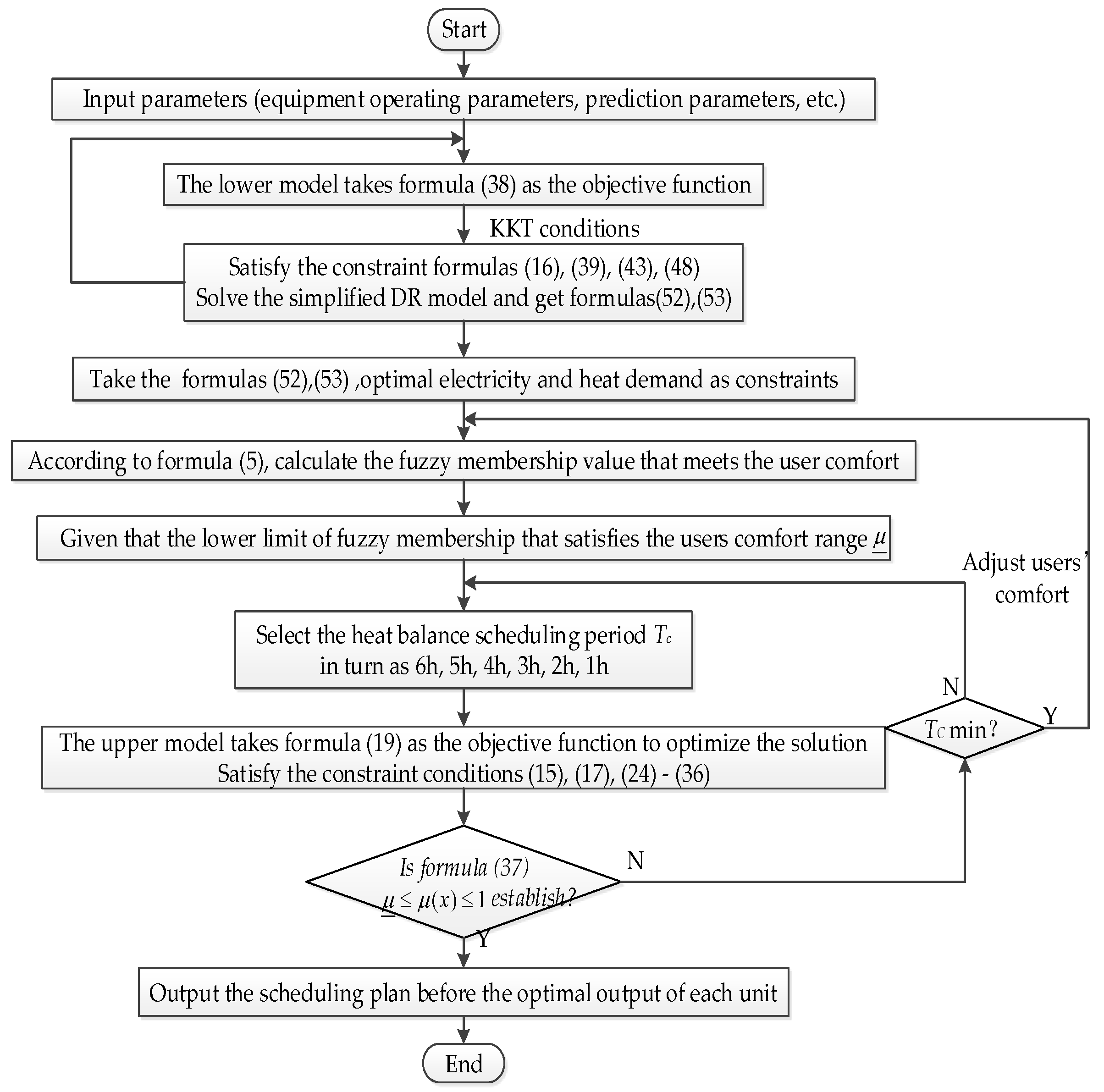
5. Bilevel Dispatch Model Optimization Strategy

5.1. Solving the Underlying Model

After the lower-level model is simplified by assumptions and nonlinear constraints, a model with Equation (38) as the objective function and Equations (16), (39), (43) and (48) as the constraint conditions are obtained. For the simplified model, we use KKT (Karush-Kukn-Tucker) optimization conditions. First, get the Lagrange function of the optimization problem:

$$\begin{array}{l}L=p_e^t{L}_{e,j}^t+p_h{L}_{h,j}^t+{\lambda }_e(L_{e,j}^t-(L_{es,j}^t+L_{e0,j}^t))+{\lambda }_h(L_{h,j}^t-R_j^t{m}_j^{set}{c}_w(T_s-T_r))\\ +{\lambda }_{eh,j}({\eta }_j{L}_{es,j}^t+{\phi }_j^t{R}_j^t-L_{h,j}^t)+{\underset{\_}{\mu }}_{R,j}(-R_j^t+{\underset{\_}{R}}_j^t)+{\overline{\mu }}_{R,j}(R_j^t-{\overline{R}}_j^t)\end{array}$$

(49)

And then:

$$\{\begin{array}{c}\frac{\partial L}{\partial L_{e,j}^t}=p_e^t+{\lambda }_e=0\hfill \\ \frac{\partial L}{\partial L_{h,j}^t}=p_h^t+{\lambda }_h=0\hfill \\ \frac{\partial L}{\partial L_{es,j}^t}=-{\lambda }_e+{\lambda }_{eh,j}{\eta }_j=0\hfill \\ \frac{\partial L}{\partial R_j^t}=-m_j^{set}{c}_w(T_s-T_r){\lambda }_h+{\phi }_j^t{\lambda }_{eh,j}-{\underset{\_}{\mu }}_{R,j}+{\overline{\mu }}_{R,j}=0\hfill \end{array}$$

(50)

where ${\lambda }_e$, ${\lambda }_h$, ${\lambda }_{eh}$, ${\underset{\_}{\mu }}_{R,j}$ and ${\overline{\mu }}_{R,j}$ are Lagrange variables, respectively.

We can get the following conclusions from Equation (50).

$$\{\begin{array}{c}{\lambda }_e=-p_e\\ {\lambda }_h=-p_h\\ {\lambda }_{eh}=\frac{{\lambda }_e}{{\eta }_j}=-\frac{p_e}{{\eta }_j}\end{array}$$

(51)

Finally, we get the optimal electricity and heat demand.

• Optimal electricity demand

  $${\displaystyle \sum L_{e,j}^t}=\{\begin{array}{c}{L}_{e0,j}^t+{\underset{\_}{L}}_{es,1}^t+{\underset{\_}{L}}_{es,2}^t+{\underset{\_}{L}}_{es,3}^t+\cdots +{\underset{\_}{L}}_{es,N_j}^t\begin{array}{cc}\begin{array}{cc}\begin{array}{cc}& \end{array}& \end{array}& p_e^t>{\xi }_{eh,1}{p}_h\end{array}\\ L_{e0,j}^t+L_{es,1}^t(R_1^t)+{\underset{\_}{L}}_{es,2}^t+{\underset{\_}{L}}_{es,3}^t+\cdots +{\underset{\_}{L}}_{es,N_j}^t\begin{array}{cc}& \underset{\_}{R}<R_1^t<\overline{R},p_e^t={\xi }_{eh,1}{p}_h\end{array}\\ L_{e0,j}^t+{\overline{L}}_{es,1}^t+{\underset{\_}{L}}_{es,2}^t+{\underset{\_}{L}}_{es,3}^t+\cdots +{\underset{\_}{L}}_{es,N_j}^t\begin{array}{cc}& {\xi }_{eh,1}{p}_h>p_e^t>{\xi }_{eh,2}{p}_h\end{array}\\ L_{e0,j}^t+{\overline{L}}_{es,1}^t+L_{es,2}^t(R_2^t)+{\underset{\_}{L}}_{es,3}^t+\cdots +{\underset{\_}{L}}_{es,N_j}^t\begin{array}{cc}& \underset{\_}{R}<R_2^t<\overline{R},p_e^t={\xi }_{eh,2}{p}_h\end{array}\\ L_{e0,j}^t+{\overline{L}}_{es,1}^t+{\overline{L}}_{es,2}^t+{\underset{\_}{L}}_{es,3}^t+\cdots +{\underset{\_}{L}}_{es,N_j}^t\begin{array}{cc}& {\xi }_{eh,2}{p}_h>p_e^t>{\xi }_{eh,3}{p}_h\end{array}\\ L_{e0,j}^t+{\overline{L}}_{es,1}^t+{\overline{L}}_{es,2}^t+L_{es,3}^t(R_3^t)+\cdots +{\underset{\_}{L}}_{es,N_j}^t\begin{array}{cc}& \underset{\_}{R}<R_3^t<\overline{R},p_e^t={\xi }_{eh,3}{p}_h\end{array}\\ \cdots \\ L_{e0,j}^t+{\overline{L}}_{es,1}^t+{\overline{L}}_{es,2}^t+{\overline{L}}_{es,3}^t+\cdots +{\overline{L}}_{es,N_j}^t\begin{array}{cc}\begin{array}{cc}\begin{array}{cc}& \end{array}& \end{array}& p_e^t<{\xi }_{eh,N_j}{p}_h\end{array}\end{array}$$

  (52)

  where ${\overline{L}}_{es}$ and ${\underset{\_}{L}}_{es}$ are the upper and lower limits of electricity-to-heat demand, respectively.
• Optimal heat demand

  $${\displaystyle \sum L_{h,j}^t}=\{\begin{array}{c}{\phi }_1^t\overline{R}+{\phi }_2^t\overline{R}+{\phi }_3^t\overline{R}+\cdots +{\phi }_{N_j}^t\overline{R}\begin{array}{cc}& p_e^t>{\xi }_{eh,1}{p}_h\end{array}\\ {\phi }_1^t{R}_1^t+{\phi }_2^t\overline{R}+{\phi }_3^t\overline{R}+\cdots +{\phi }_{N_j}^t\overline{R}\begin{array}{cc}& \underset{\_}{R}<R_1^t<\overline{R},p_e^t={\xi }_{eh,1}{p}_h\end{array}\\ {\phi }_1^t\underset{\_}{R}+{\phi }_2^t\overline{R}+{\phi }_3^t\overline{R}+\cdots +{\phi }_{N_j}^t\overline{R}\begin{array}{cc}& {\xi }_{eh,1}{p}_h>p_e^t>{\xi }_{eh,2}{p}_h\end{array}\\ {\phi }_1^t\underset{\_}{R}+{\phi }_2^t{R}_2^t+{\phi }_3^t\overline{R}+\cdots +{\phi }_{N_j}^t\overline{R}\begin{array}{cc}& \underset{\_}{R}<R_2^t<\overline{R},p_e^t={\xi }_{eh,2}{p}_h\end{array}\\ {\phi }_1^t\underset{\_}{R}+{\phi }_2^t\underset{\_}{R}+{\phi }_3^t\overline{R}+\cdots +{\phi }_{N_j}^t\overline{R}\begin{array}{cc}& {\xi }_{eh,2}{p}_h>p_e^t>{\xi }_{eh,3}{p}_h\end{array}\\ {\phi }_1^t\underset{\_}{R}+{\phi }_2^t\underset{\_}{R}+{\phi }_3^t{R}_3^t+\cdots +{\phi }_{N_j}^t\overline{R}\begin{array}{cc}& \underset{\_}{R}<R_3^t<\overline{R},p_e^t={\xi }_{eh,3}{p}_h\end{array}\\ \cdots \\ {\phi }_1^t\underset{\_}{R}+{\phi }_2^t\underset{\_}{R}+{\phi }_3^t\underset{\_}{R}+\cdots +{\phi }_{N_j}^t\underset{\_}{R}\begin{array}{cc}& p_e^t<{\xi }_{eh,N_j}{p}_h\end{array}\end{array}$$

  (53)

In Equations (52) and (53), we have made the following assumptions: The efficiency of the consumer’s electrical conversion equipment is ${\eta }_1\ge {\eta }_2\ge \dots \ge {\eta }_{N_j}$. In addition, in order to express the relationship between time-of-use electricity price $p_e^t$ and heat price ${\chi }^2$$p_h$, a variable ${\xi }_{eh,j}=\frac{{\eta }_j{c}_w{m}_j^{set}(T_s-T_r)}{{\phi }_j^t}$ is defined, which can also be simplified to ${\xi }_{eh,j}={\eta }_j\frac{T_s-T_r}{T_{in}-T_{out}}$.

5.2. Bilevel Optimized Operation Strategy

The optimized electricity-heat integrated system model established in this paper includes two objective functions: Optimal operating cost on the energy supply side and minimizing user cost. It is a two-tier dispatch model covering the supply and demand side.

The bilevel model introduces user DR, and takes the minimum cost on the user side as the optimization goal. By simplifying the heating network model and optimizing the KKT conditions, the most economical piecewise linear function of electricity and heat demand is made according to the relationship between time-of-use electricity prices and heat prices. Taking the optimal operating cost on the energy supply side as the upper-level optimization goal, and using the piecewise function as the constraint of the upper-level optimization model to solve the upper-level optimization problem, turning the bilevel optimization problem into a single-layer optimization problem. While ensuring the lowest energy purchase cost for users, it also ensures the energy supply economy of the energy supply side units.

The solution flow chart of the bilevel dispatch model of the electricity-heat integrated system established in this paper is shown in Figure 4. The solution is solved by the primal dual interior Point method [37,38,39]. This method is robust, insensitive to the initial value selection, and converges rapidly. When solving large-scale systems, the number of iterations varies little with greatly increased constraints.

6. Simulation Analysis Discussion

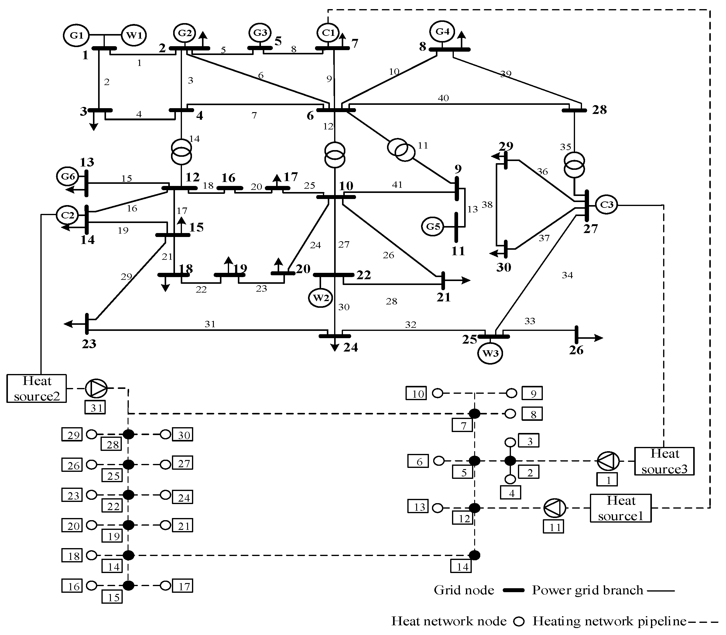
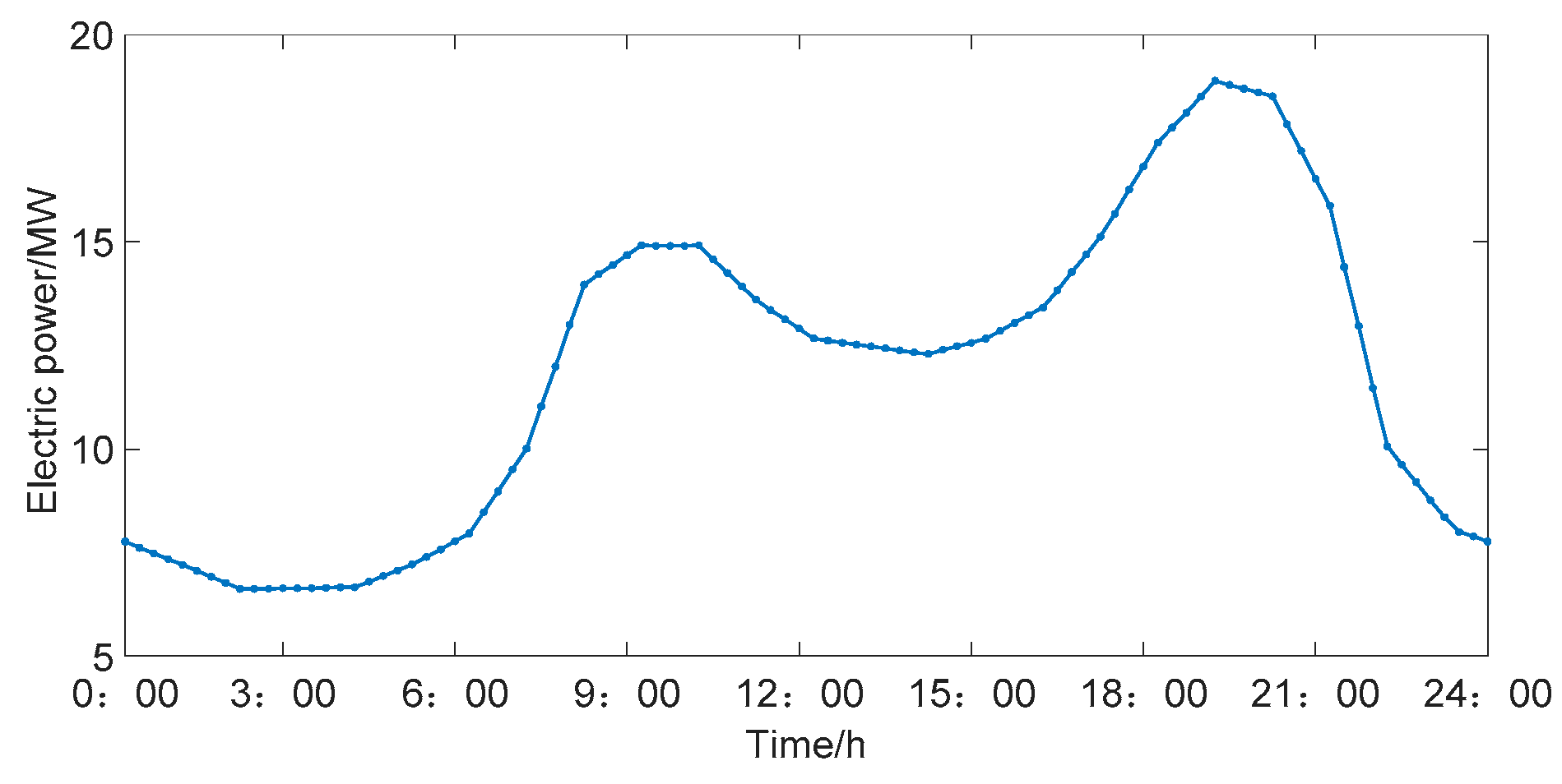
6.1. Example System and Simulation Parameters

The electricity-heat integrated simulation system adopted is composed of the IEEE30 node power network and the 31 node heating network. As shown in Figure 5, the power network includes 30 buses, 41 transmission lines, 24 loads, 3 wind power units, 6 thermal power units, and 3 CHP units. Nodes 1, 11, and 31 of the heat supply network are coupled with grid nodes 27, 7, and 14 through CHP. Considering the difference of electric and thermal time scales, the dispatching time interval of the power system is set as 15 min, and that of the thermal system is 1 h. As thermoelectric coupling equipment, the dispatching time interval of CHP’s power supply and heating is defined as 1 h.

The total power load is shown in Figure 6.

The user thermal demand curve based on the most comfortable temperature can be obtained through the temperature difference between the supply and the return water of the pipeline in different periods as well as in Equations (1)–(3), as shown in Figure 7.

When users relax their requirements on thermal comfort and take fuzzy membership function as the standard to measure the thermal comfort of users, the thermal demand of users can fluctuate within a certain range. We use the minimum thermal comfort standard of 3000 users to get the envelope of the thermal demand of the electricity-heat integrated system based on the thermal comfort of users, which is the total thermal load, as shown in Figure 8. Through the heat demand envelope, we can adjust the thermal load in a specific period of time, and the thermal output of the unit only needs to fall within the envelope band, which can increase the flexibility of the system dispatch.

Heating network parameters are shown in

Table 1. Parameters of the heating network.

Parameter	Value	Parameter	Value
$c_w$	4200	${\eta }_{e,cj}$	0.3
$l$	200	${\eta }_{h,cj}$	0.75
h	0.25	${\eta }_{gb,j}$	0.95

and unit parameters are shown in

Table 2. Parameters of the generators and initial value setting.

Unit	Parameter	Value
G1, G4	$a_e/b_e/c_e$	0.097/50/0
	$P_{e,g1}^{\max }$	3
G2, G5	$a_e/b_e/c_e$	0.096/47/0
	$P_{e,g2}^{\max }$	3
G3, G6	$a_e/b_e/c_e$	0.094/45/0
	$P_{e,g3}^{\max }$	3
C1	$a_e/b_e/c_e$	0.02/100/0
	$a_h/b_h/c_h$	0.02/100/0
	$P_{e,c1}^{\max }$/$P_{h,c1}^{\max }$	3/6
C2	$a_e/b_e/c_e$	0.015/95/0
	$a_h/b_h/c_h$	0.015/95/0
	$P_{e,c2}^{\max }$/$P_{h,c2}^{\max }$	3/6
C3	$a_e/b_e/c_e$	0.01/90/0
	$a_h/b_h/c_h$	0.01/90/0
	$P_{e,c3}^{\max }$/$P_{h,c3}^{\max }$	3/6
W1, W2, W3	$P_{e,w1}^{\max }$/$P_{e,w2}^{\max }$/$P_{e,w3}^{\max }$	0.5/0.5/0.5

.

When the method in this paper is applied to a larger scale practical system, the number of nodes to be processed increases or the scale of the calculation example becomes larger and more complicated. Because of the increase in data to be processed, the simulation execution will definitely increase the amount of calculation compared with the small-scale calculation example. However, the applicability of the algorithm itself will not change due to the scale of the calculation example, and the objective function, constraint conditions, and simulation process proposed in this paper will not change. Since Equations (24)–(29) are applicable to n-node systems, only different initial data are needed due to the difference in the node admittance matrix and the topology constraints, for example, the grid line parameters, node admittance matrix and load distribution parameters of the standard model of n-node distribution network (as Figure 5 and Figure 6 and reference [40] show), and the heat supply network pipe length, the heat transfer coefficient, the specific heat capacity of water, and the load distribution of the n-node thermal system (as Figure 8, Table 1 and Table 2 show). Therefore, the method proposed in this paper can be extended to the n-node power system

6.2. Simulation Analysis without Considering DR

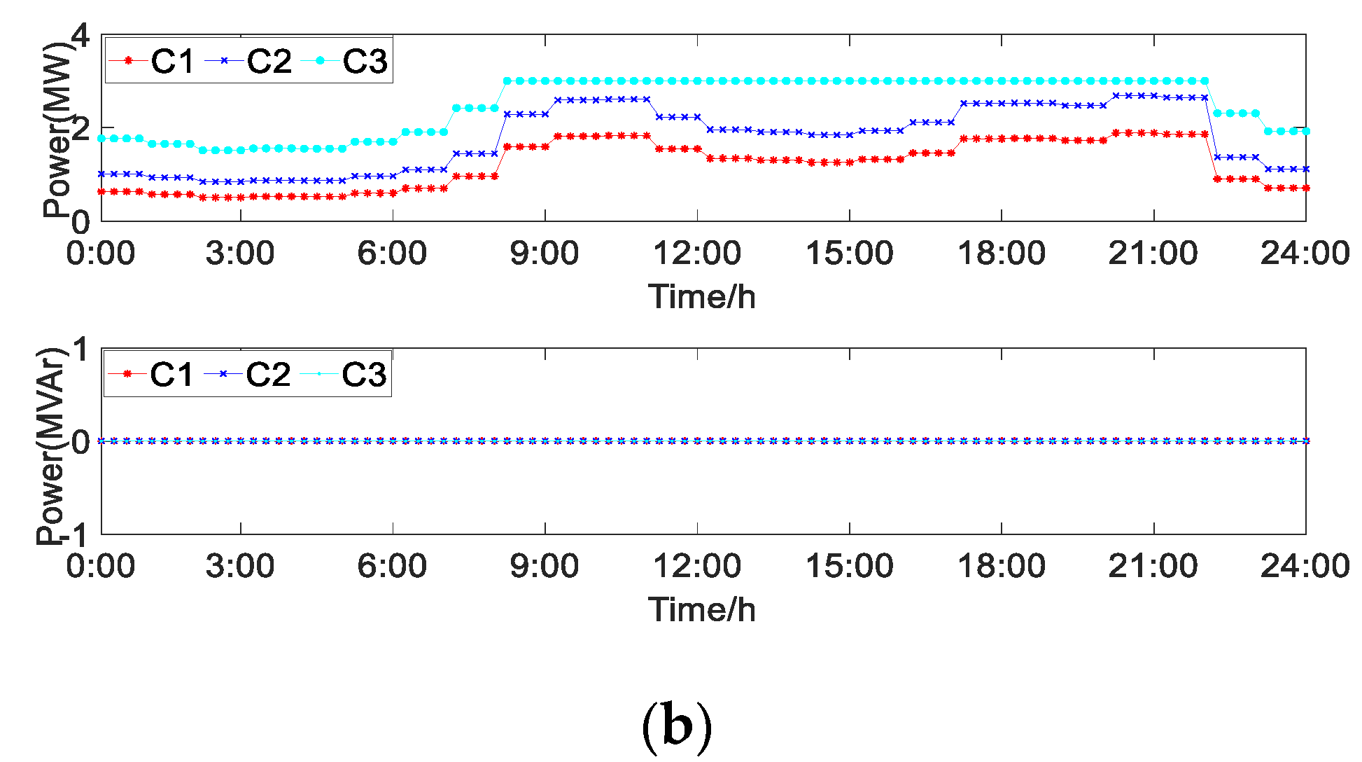
6.2.1. Comparison with Traditional Centralized Algorithms

Based on the typical days in the Liaoning Province of China without considering the output of the wind turbine, the optimization results are shown in Figure 9 and Figure 10. Comparing the two scenarios, it can be seen that the results obtained by the traditional centralized algorithm [41] do not involve the reactive power output of the unit, and the optimization results obtained by considering the specific electrical network topology have a large deviation from the unit output results obtained by the traditional centralized algorithm. From the comparison of the optimization results, it can be seen that the optimization of the unit reactive power output has a great impact on the optimal dispatch results of the unit, which proves that the traditional centralized method does not consider the actual network topology and has an optimization deviation. In a word, the optimization model and the optimization strategy proposed in this paper are more practical.

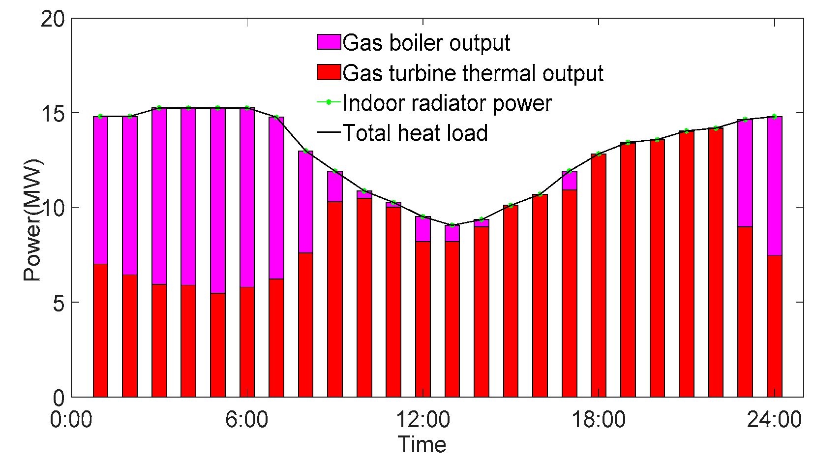
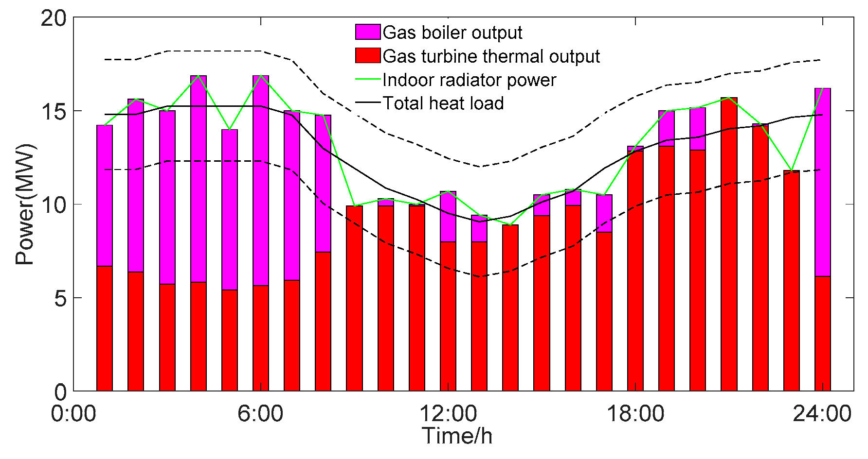
6.2.2. The Influence of the Heat Demand Envelope on Unit Output

Taking 1 h as the dispatch time interval, we get the change in the heat output of the unit by considering the heat demand envelope, as shown in Figure 11 and Figure 12. Comparing the two scenarios, it can be seen that when the heat demand envelope is not considered, the total power of the radiator and the total heat load must be balanced in real time, so the output of the CHP unit is obviously not flexible enough. When considering the envelope of heat demand, the heat output of the unit only needs to fall within the envelope, and the adjustment range of the CHP unit can be increased. In this paper, the user thermal demand envelope can optimize the output of the unit and increase the flexibility of system dispatch.

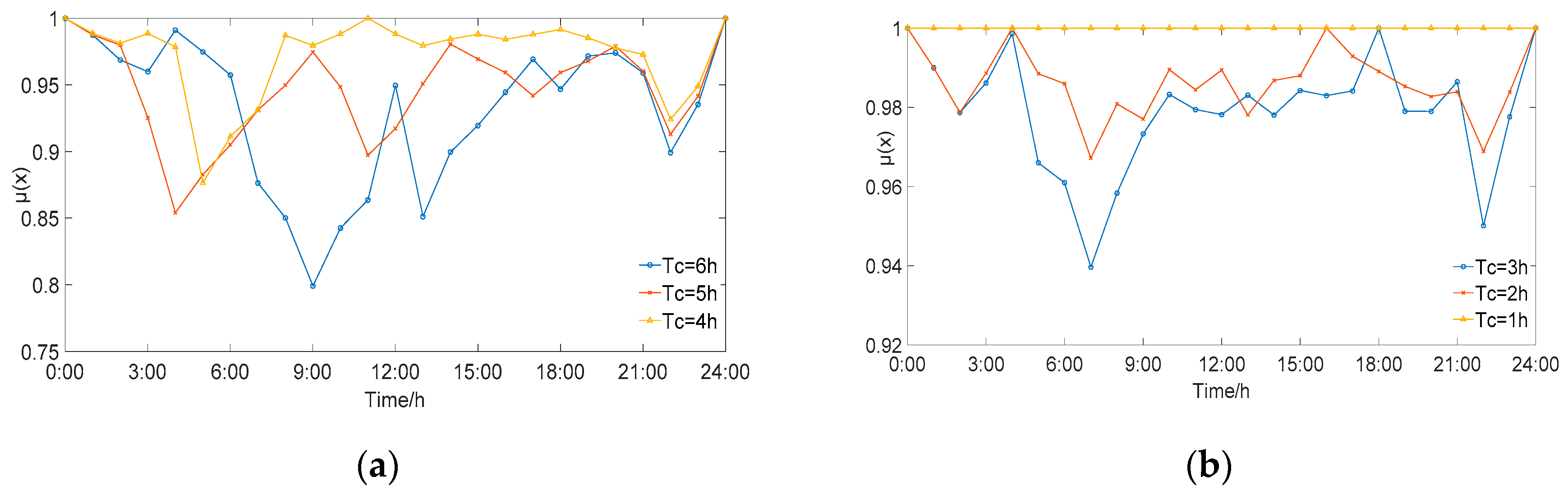
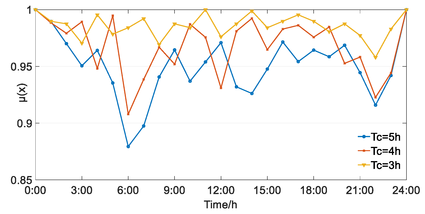
6.2.3. The Influence of Thermal Balance Cycle on Thermal Comfort

Figure 13 shows that the value of $\mu$ changes when the heat balance cycle is 6 h, 5 h, 4 h, 3 h, 2 h, and 1 h. It can be seen from Figure 13 that as the thermal balance cycle continues to decrease, the amount of change in the fuzzy membership value based on the user’s thermal comfort gets smaller and smaller until the requirement is met. Traditional units generally take a thermal balance cycle of 1 h, and through simulation analysis, we found that users’ thermal comfort needs can be met when the thermal balance cycle is less than 3 h. Moreover, the larger the thermal balance cycle, the more flexible the unit’s output and the more an optimal energy dispatch can be achieved. Therefore, we define the optimal thermal balance cycle value as 3 h.

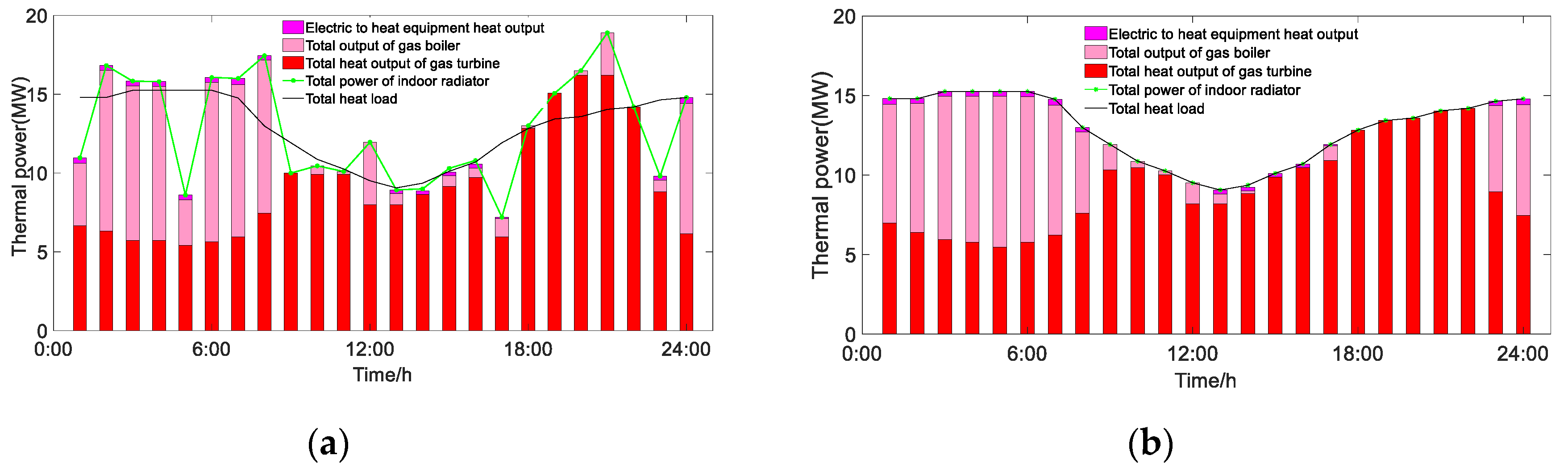
6.2.4. The Influence of the Heat Balance Cycle on Unit Output

The electrical power balance is shown in Figure 14 and the thermal power balance is shown in Figure 15.

When $T_c$ = 1 h, in order to maintain the balance of power supply and demand, the electricity-heat integrated system purchases electricity from the superior power grid during the peak electricity price period from 19:00–21:00. When $T_c$ = 3 h, within the thermal comfort range of the user, the thermal energy only needs to meet the supply and demand balance of the total heat in the heat balance cycle. Therefore, the electricity-heat integrated system increases the output of the CHP unit during peak electricity consumption during the dispatch cycle, thereby reducing the power purchase of the superior power grid during peak hours. The cost of electricity purchase is reduced, and the economy of the system operation is improved.

6.3. Considering DR Simulation Analysis

By considering the user’s DR, we obtain the user’s DR to the electricity price and changes in unit thermal output after user DR, as shown in Figure 16 and Figure 17.

It can be seen from Figure 16 that users’ DR mainly uses wind power through electricity-to-heat equipment for heating during low electricity prices. In normal electricity prices, due to the difference in the efficiency of users’ electricity-to-heat equipment, selective electric heating is performed to reduce the output of heating equipment. Figure 17 shows that the DR user’s electricity-to-heat equipment does not take any action at the peak electricity price, because the peak electricity price is too high and it is not cost-effective for users to choose electricity-to-heat. The conclusion can be drawn that the user’s DR reduces the total energy purchase cost through the price difference between electricity and heat.

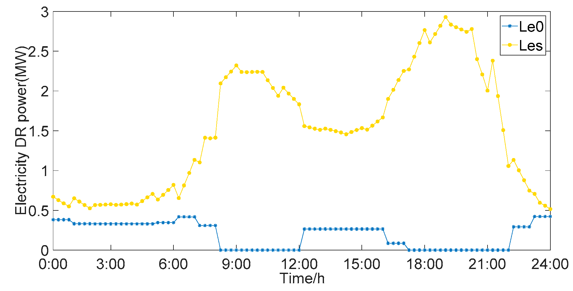
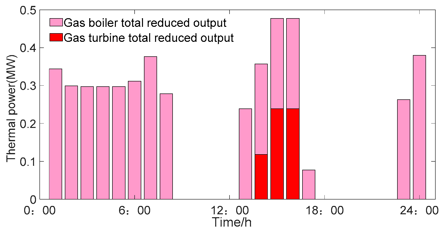
6.3.1. The Influence of DR on the Heat Balance Cycle

It can be seen from Figure 18 that user DR changes the optimal heat balance cycle of the electricity-heat integrated system from 3 h to 4 h, since the user’s DR increases the diversity of heat production equipment through the output of electric-to-heat equipment. Heat production also provides space for the upper limit of the total heating output, and DR electricity can also be obtained through the unit’s electrical output, which increases the output range of the unit and improves the overall flexibility of the unit.

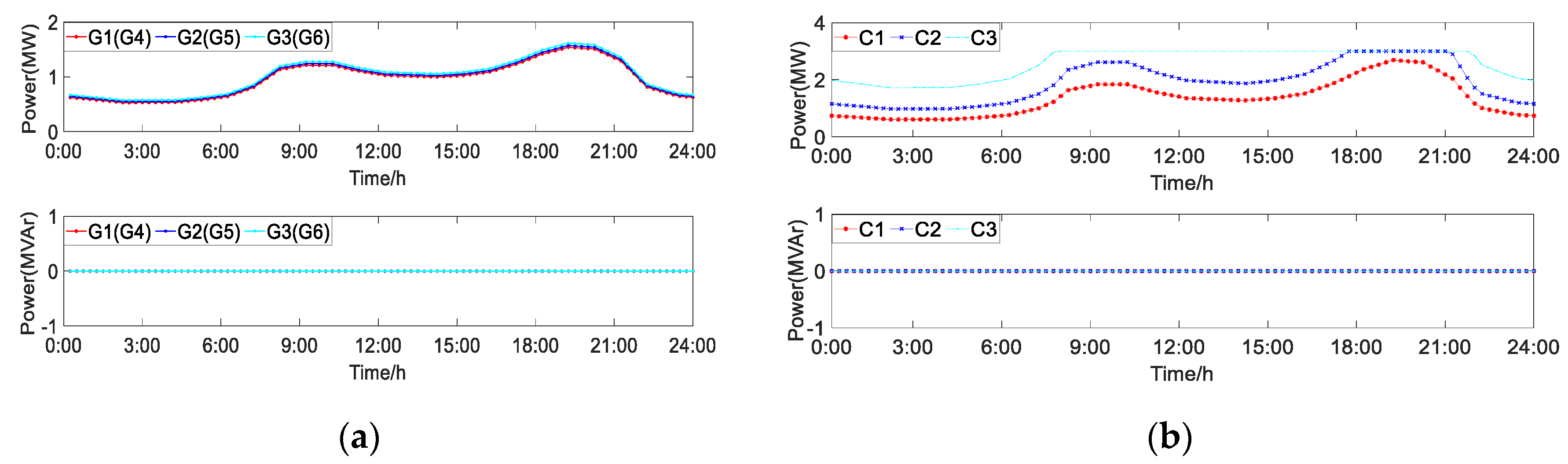
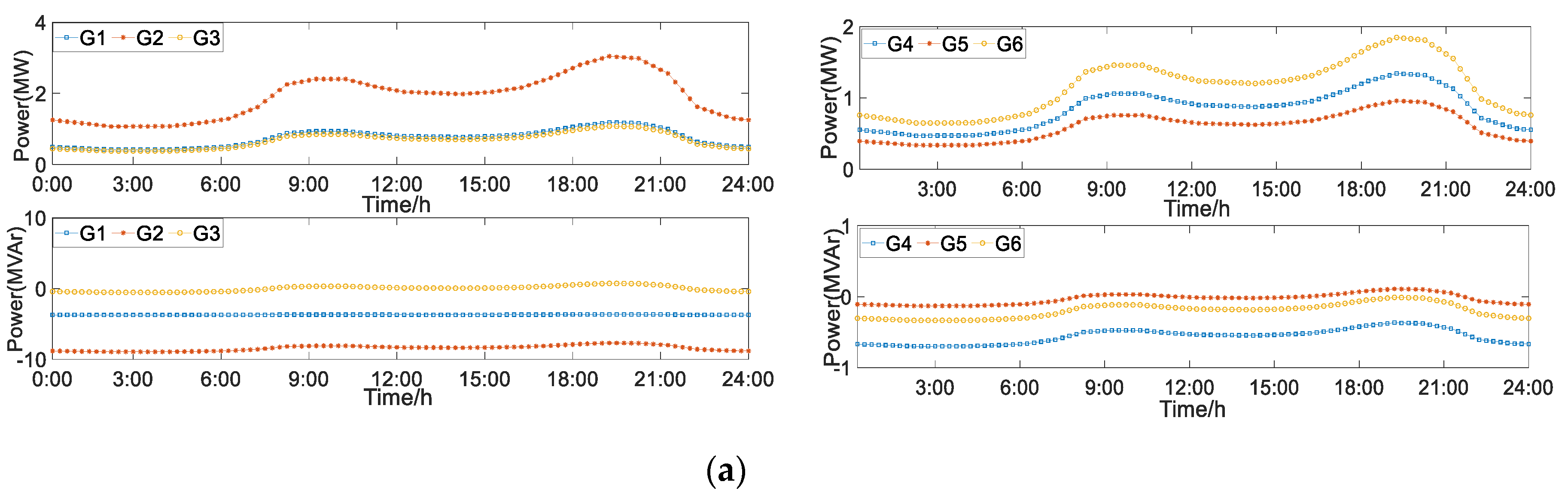
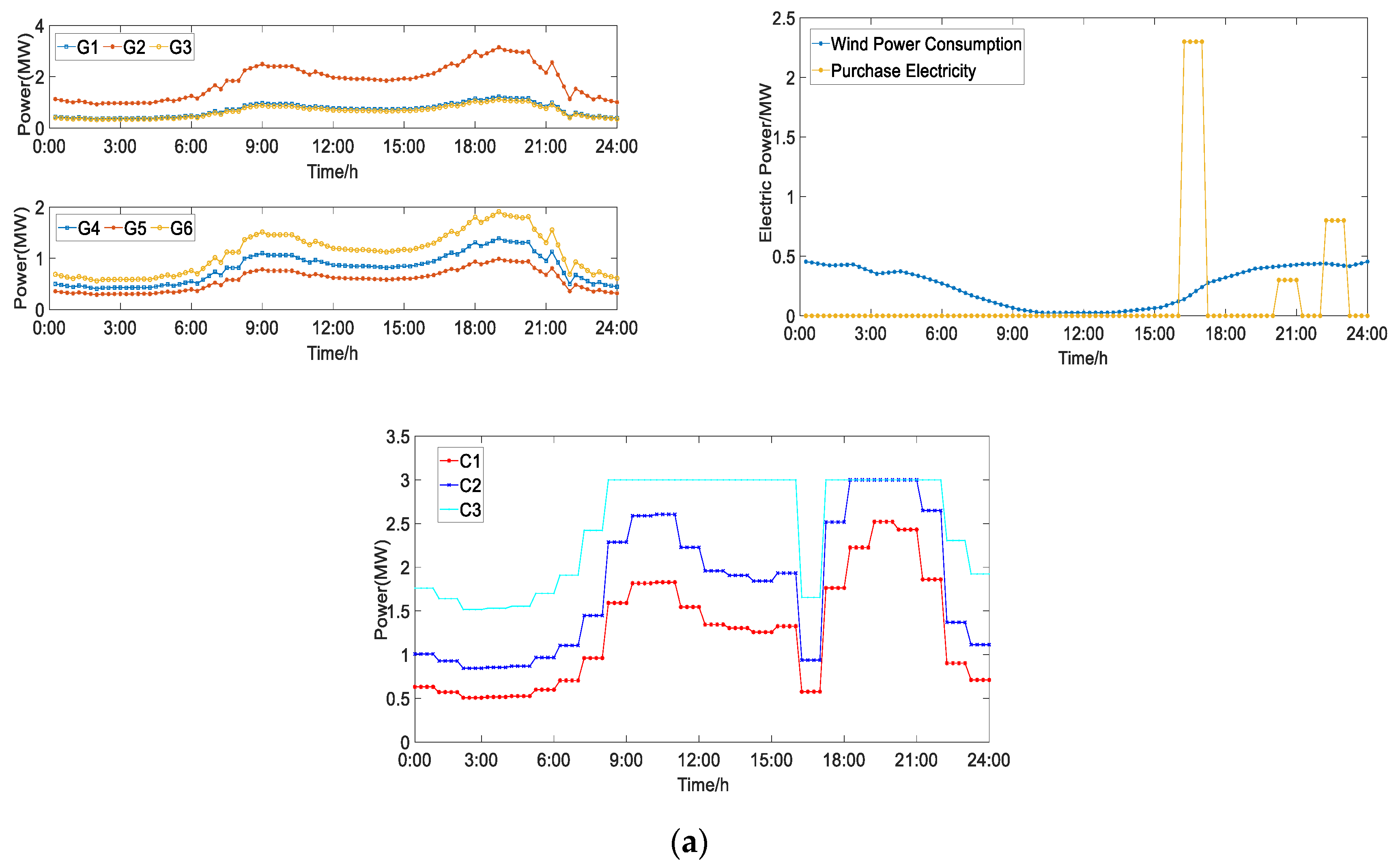
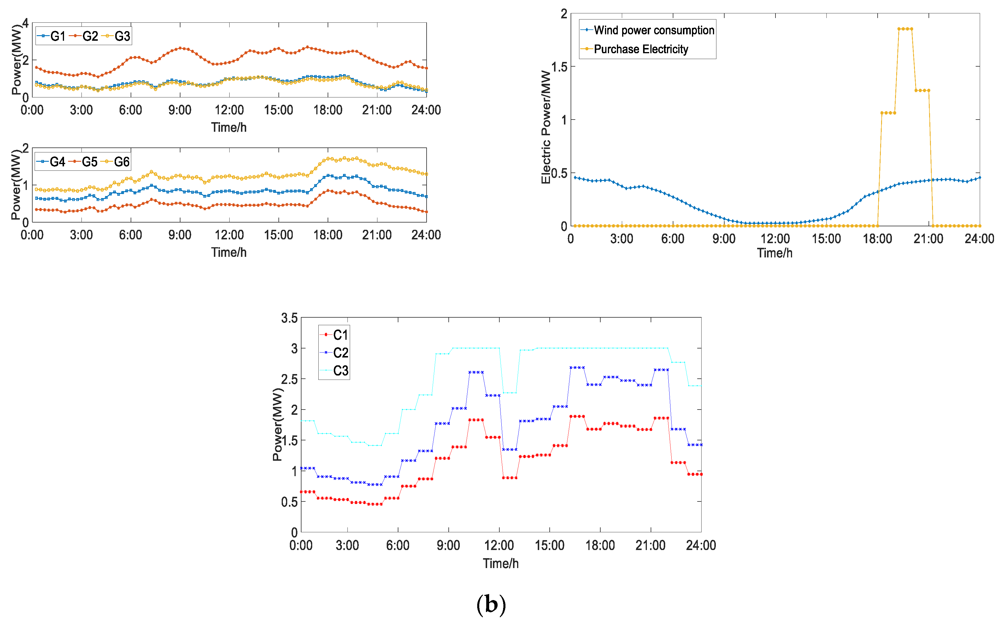
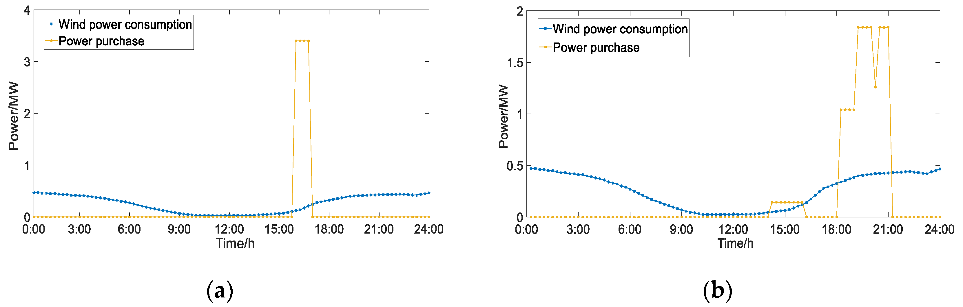
6.3.2. The Influence of DR on Unit Output

The wind power consumption and power purchase is shown in Figure 19 and the heat power balance is shown in Figure 20. The main difference between the unit output after considering the DR when $T_c$ = 4 h and not considering the DR when $T_c$ = 3 h, is the increase of the optimal heat balance cycle $T_c$, which will increase the flexibility of the unit output for the reason that the supply of heat energy only needs to meet the total heat balance during the heat balance cycle and satisfy the user’s thermal comfort. We found that the electricity purchase phenomenon considering the DR when $T_c$ = 4 h mainly occurs at the normal electricity price at 17:00, as well as when the demand for electricity purchase is large. Meanwhile, regardless of the DR when $T_c$ = 3 h, there is a small amount of power purchase during peak hours which greatly reduces the economic efficiency of the production capacity of the electricity-heat integrated system due to the high price of electricity during peak hours. In addition, the increased DR users will use the valley hour electricity price to convert electricity to heat, increase wind power consumption, and effectively use the wind power surplus to reduce users’ energy purchase costs while also increasing the economics of energy supply side capacity.

The main difference between the unit output after considering the DR when $T_c$ = 1 h and regardless of the DR when $T_c$ = 1 h, is that the total output of wind turbines has been increased during the low price of the DR, for the users who participate in the DR will increase the electricity consumption during the low price period to convert electricity into heat to absorb excess wind power. In addition, due to the investment in electric-to-heat equipment, the heat output of gas boilers and gas turbine units on the energy supply side is reduced, thereby improving the production economy of the electricity-heat integrated system. Moreover, in the case of considering users’ DR, the system will choose to purchase electricity from the superior power grid to convert electricity into heat according to the optimization results of the optimal electric-heating demand, so as to reduce the electric heating output of the gas turbine, improve the economy of users and increase the flexibility of the unit. It is obvious that, in the case of considering the DR of users, the system will perform selective electricity conversion at normal electricity prices based on the optimal electric-heating demand optimization result, which also improves the economic efficiency of user energy consumption.

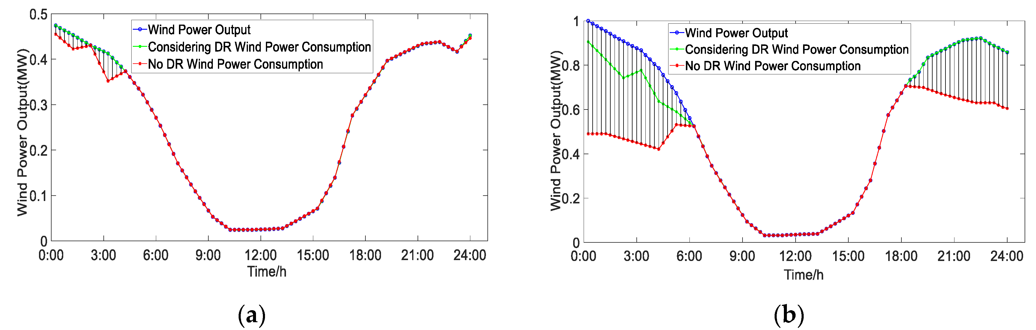
6.3.3. The Influence of DR on Wind Power Consumption

In order to analyze the impact of the electricity-heat integrated system considering user DR on wind power consumption, we designed the upper limit of total wind power output of 0.5 MW and the upper limit of total wind power output of 1 MW for analysis, and compared the consumption of wind power that responds to user DR under different wind power penetration rates.

According to the wind power consumption results in Figure 21, under the situation that the upper limit of the total output of wind power is 0.5 MW, the complete consumption of wind energy can be achieved in consideration of user DR, while the phenomenon of wind abandonment occurs in the case of no DR. In the case of the upper limit of the total output of wind power being 1 MW, the situation of taking into account the user’s DR will also cause wind abandonment during the low electricity consumption situation, but compared with the case without considering the user’s DR, the consumption of wind power has been significantly improved.

It is concluded that the corresponding system with demand can effectively absorb wind energy compared with the system without DR, which can effectively reduce the electricity output of the unit and the power supply cost. Furthermore, the effective use of green energy has contributed to sustainable development and energy cleaning.

6.3.4. The Influence of DR and Optimal Heat Balance Cycle on Economy

In order to analyze the impact of user DR on economy, we set up several comparison scenarios, and the obtained cost scenarios are shown in

Table 3. Economic cost comparison.

Case	State	${\mathit{P}}_{\mathit{e},\mathit{w}}^{\mathbf{max}}$ = 0.5 MW			${\mathit{P}}_{\mathit{e},\mathit{w}}^{\mathbf{max}}$ = 1 MW
		Wind Power Consumption (MW·h)	Power Purchase Cost (Ten Thousand Yuan)	Total Cost (Ten Thousand Yuan)	Wind Power Consumption (MW·h)	Total Cost (Ten Thousand Yuan)
DR	×	6.026	0.312	21.1486	9.232	21.052
$T_c$	1 h
DR	×	6.052	0.181	21.0271	9.261	21.931
$T_c$	3 h
DR	√	6.136	0.307	21.126	12.087	20.947
$T_c$	1 h
DR	√	6.182	0.177	21.0201	12.134	20.842
$T_c$	4 h

.

It can be seen that, when $P_{e,w}^{\max }$ = 0.5 MW, considering that DR has no obvious impact on the total cost, the heat balance cycle is the main factor affecting the total cost. When $P_{e,w}^{\max }$ = 1 MW, the wind power consumption including DR increases significantly. The DR and the optimal heat balance cycle have an important effect on the cost. Regarding the impact of total cost, DR mainly uses surplus wind power to improve economy, as well as the optimal thermal balance cycle mainly using thermal inertia to reduce costs by increasing the flexibility of the unit and reducing peak power purchases under the premise of satisfying the user’s thermal comfort.

7. Conclusions

In this paper, a bilevel model of time-scale economic dispatch of the electricity-heat integrated system is proposed, which includes the economic dispatch model of the upper level energy supply side and the minimum energy purchase cost model of the lower level user side. Finally, the bilevel optimization problem is transformed into a single-layer optimization problem by the KKT condition. The simulation result shows that the proposed economic dispatch model can make full use of the difference in dynamic characteristics between electric and heating networks, and effectively improve the economy of the energy supply. The DR model can effectively promote the wind power consumption, increase the heat balance cycle, improve the flexibility of the unit operation, and achieve significant economic benefits.

In the economic research of the electricity-heat integrated system, the fuzzy membership index based on users’ thermal comfort is innovatively put forward to reflect the relationship between heating power and users’ thermal comfort, and the concept of the user heat demand envelope band is proposed. The heating power can be within the envelope band, which makes the output of the thermal power unit more flexible. However, the disadvantage of this paper is that it simplifies the specific structure of the thermal network, only considering the total heat balance of the heat supply network in the heat balance cycle. Due to the transmission delay of the thermal system, the supply and demand can be staggered in the time scale and the heating network structure considering the transmission delay is an important direction for subsequent research.

In addition, the DR of this paper is different from other studies, taking into account the impact of the DR of electrothermal coordination on the economic cost of the entire system. Moreover, this paper only considers the DR of the residential user load, so that multiple load types (such as residential, industrial, commercial, office) can be considered to carry out collaborative DR according to their load differences in the further study.

References

1. Yin, S.R.; Ai, Q.; Zeng, S.Q. Research Challenges and Prospects of Multi-energy Distributed Optimization of Energy Internet. Power Syst. Technol. 2018, 5, 1359–1369. [Google Scholar]
2. Zhou, R.J.; Chao, D.X.; Li, X.J. Space Coupled Particle Swarm Optimization Algorithm and IES-CCHP Regional Joint Dispatch under Peak-Valley Electricity Prices. Electr. Power Autom. Equip. 2016, 36, 11–17. [Google Scholar]
3. Ameri, M.; Besharati, Z. Optimal Design and Operation of District Heating and Cooling Networks with CCHP Systems in a Residential Complex. Energy Build. 2016, 110, 135–148. [Google Scholar] [CrossRef]
4. Gu, W.; Wang, Z.; Wu, Z. An Online Optimal Dispatch Schedule for CCHP Microgrids Based on Model Predictive Control. IEEE Trans. Smart Grid 2016, 99, 1–11. [Google Scholar]
5. Chang, C.S.; Fu, W. Stochastic Multi Objective Generation Dispatch of Combined Heat and Power Systems. IEEE Proc. Gener. Transm. Distrib. 2002, 145, 583–591. [Google Scholar] [CrossRef]
6. Moradi, H.; Moghaddam, M.P.; Moghaddam, I.G. Opportunities to Improve Energy Efficiency and Reduce Greenhouse Gas Emissions for a Cogeneration Plant. In Proceedings of the 2010 IEEE International Energy Conference, Manama, Bahrain, 18–22 December 2010; pp. 785–790. [Google Scholar]
7. Dai, Y.H.; Chen, L.; Min, Y. Optimal Dispatch of Combined Operation of Wind Farm and Cogeneration with Heat Storage. Proc. Chin. Soc. Electr. Eng. 2017, 37, 3470–3479. [Google Scholar]
8. Chen, X. Increasing the Flexibility of Combined Heat and Power for Wind Power Integration in China: Modeling and Implications. IEEE Trans. Power Syst. 2015, 30, 1848–1857. [Google Scholar] [CrossRef]
9. Fragaki, A.; Andersen, A.N. Conditions for Aggregation of CHP Plants in the UK Electricity Market and Exploration of Plant Size. Appl. Energy 2011, 88, 3930–3940. [Google Scholar] [CrossRef]
10. Li, Z.; Wu, W.; Wang, J.; Zhang, B.; Zheng, T. Transmission-Constrained Unit Commitment Considering Combined Electricity and District Heating Networks. IEEE Trans. Sustain. Energy 2016, 7, 480–492. [Google Scholar] [CrossRef]
11. Olaia, E. Energy, Environmental and Economic Analysis of Air-to-Air Heat Pumps as an Alternative to Heating Electrification in Europe. Energies 2020, 13, 3939. [Google Scholar]
12. Pei, W.; Deng, W.; Shen, Z.Q. Energy Coordination and Optimization of Hybrid Microgrid with Renewable Energy and Combined Heat and Power. Autom. Electr. Power Syst. 2014, 38, 9–15. [Google Scholar]
13. Yu, D.Y.; Liang, J.; Han, X.S.; Zhao, J.G. Profiling the Regional Wind Power Fluctuation in China. Energy Policy 2011, 39, 299–306. [Google Scholar] [CrossRef]
14. Anwar, M.B.; Qazi, H.W.; Burke, D.J.; Malley, M.J.O. Harnessing the Flexibility of Demand-Side Resources. IEEE Trans. Smart Grid 2019, 10, 4151–4163. [Google Scholar] [CrossRef]
15. Tang, W.; Gao, F. Optimal Operation of Household Micro-Grid Day-Ahead Energy Considering User Satisfaction. High Volt. Eng. 2017, 43, 140–148. [Google Scholar]
16. Dou, C.; Meng, C.; Yue, W.; Zhang, B. Double-Deck Optimal Schedule of Micro-Grid Based on Demand-Side Response. IET Renew. Power Gener. 2019, 13, 847–855. [Google Scholar] [CrossRef]
17. Michał, T.; Robert, S. Buildings and a district heating network as thermal energy storages in the district heating system. Energy Build. 2018, 179, 49–56. [Google Scholar]
18. Semikashev, V.V. Heat comfort of the population of Russia. Stud. Russ. Econ. Dev. 2010, 21, 393–402. [Google Scholar] [CrossRef]
19. Zhu, C.Z.; Lu, S.; Zhou, J.H. Day-Ahead Economic Dispatch of Integrated Energy System Based on Electricity-Heat Time Scale Balance. Electr. Power Autom. Equip. 2018, 6, 138–143. [Google Scholar]
20. Ge, W.C.; Li, P.; Sun, S.L.; Liu, A.M.; Li, J.J. Pre-Day Coordinated Optimal Control of Large-Scale Electro-thermal Internet Based on the Response of Heating Temperature Demand of Thermal Users. In Proceedings of the 2019 IEEE Innovative Smart Grid Technologies—Asia (ISGT Asia), Chengdu, China, 21–24 May 2019; pp. 3567–3572. [Google Scholar]
21. Stamminger, R.; Broil, G.; Pakula, C.; Jungbecker, H.; Braun, M.; Rüdenauer, I.; Wendker, C. Synergy potential of smart appliances. Rep. Smart A Proj. 2008, D2.3, 1949–3053. [Google Scholar]
22. Wang, J. Planning and Optimized Operation of Regional Integrated Energy System; Southeast University: Nanjing, China, 2017. [Google Scholar]
23. Vahedipour-Dahraie, M.; Rashidizadeh-Kermani, H.; Najafi, H.R. Stochastic Security and Risk-Constrained Scheduling for an Autonomous Micro-Grid with Demand Response and Renewable Energy Resources. IET Renew. Power Gener. 2017, 11, 1812–1821. [Google Scholar] [CrossRef]
24. Chen, J.S. Research on Demand Response Technology for Smart Power Consumption and Household Power Consumption Strategy; Chongqing University: Chongqing, China, 2014. [Google Scholar]
25. Xu, B.; Liu, H.X. Optimal Dispatch of Regional Microgrid Based on Demand Response. J. Electr. Power Sci. Technol. 2018, 33, 132–140. [Google Scholar]
26. Aalami, H.A.; Moghaddam, M.P.; Yousefi, G.R. Modeling and Prioritizing Demand Response Programs in Power Markets. Electr. Power Syst. Res. 2010, 80, 426–435. [Google Scholar] [CrossRef]
27. Mognaddam, M.P.; Abdollahi, A.; Rashidinejad, M. Flexible Demand Response Programs Modeling in Competitive Electricity Markets. Appl. Energy 2011, 88, 3257–3269. [Google Scholar] [CrossRef]
28. Lynch, M.; Nolan, S.; Devine, M.T. The Impacts of Demand Response Participation in Capacity Markets. Appl. Energy 2019, 250, 444–451. [Google Scholar] [CrossRef] [Green Version]
29. Logenthiran, T.; Srinivasan, D.; Shun, T.Z. Demand Side Management in Smart Grid Using Heuristic Optimization. IEEE Trans. Smart Grid 2012, 3, 1244–1252. [Google Scholar] [CrossRef]
30. Yang, X.; Zhang, Y.; He, H.; Ren, S.; Weng, G. Real-Time Demand Side Management for a Microgrid Considering Uncertainties. IEEE Trans. Smart Grid 2019, 10, 3401–3414. [Google Scholar] [CrossRef]
31. Wang, J.H.; Bloyd, C.N.; Zhao, G.H. Demand Response in China. Energy 2010, 35, 1592–1597. [Google Scholar] [CrossRef]
32. Xue, Y.T.; Chen, Y.C.; Li, X.W. A Joint Peak-Valley Time-Of-Use Electricity Price Model Based on Customer Satisfaction and Ramsey Pricing Theory. Power Syst. Prot. Control 2018, 46, 122–128. [Google Scholar]
33. Zou, Y.Y.; Yang, L.; Feng, L. Microgrid Heat and Power Coordinated Dispatch Considering Two-Dimensional Controllability of Heat Load. Autom. Electr. Power Syst. 2017, 41, 13–19. [Google Scholar]
34. Duquette, J.; Rowe, A.; Wild, P.; Yan, J. Thermal Performance of a Steady State Physical Pipe Model for Simulating District Heating Grids with Variable Flow. Appl. Energy 2016, 178, 383–393. [Google Scholar] [CrossRef]
35. Zhang, X.; Shahidehpour, M.; Alabdulwahab, A.; Abusorrah, A. Optimal Expansion Planning of Energy Hub with Multiple Energy Infrastructures. IEEE Trans. Smart Grid 2015, 6, 2302–2311. [Google Scholar] [CrossRef]
36. Moeini-Aghtaie, M.; Dehghanian, P.; Fotuhi-Firuzabad, M.; Abbaspour, A. Multi-Gent Genetic Algorithm: An Online Probabilistic View on Economic Dispatch of Energy Hubs Constrained by Wind Availability. IEEE Trans. Sustain. Energy 2014, 5, 699–708. [Google Scholar] [CrossRef]
37. Stephen, B.; Lieven, V. Convex Optimization; Cambridge University Press: Cambridge, UK, 2004. [Google Scholar]
38. Nocedal, J.; Stephen, J.W. Numerical Optimization, 2nd ed.; Springer: Berlin, Germany, 2006. [Google Scholar]
39. Yildirim, E.A.; Wright, S.J. Warm-Start Strategies in Interior-Point Methods for Linear Programming. SIAM J. Optim. 2002, 12, 782–810. [Google Scholar] [CrossRef]
40. Mousavi, O.A.; Cherkaoui, R. Investigation of P–V and V–Q Based Optimization Methods for Voltage and Reactive Power Analysis. Int. J. Electr. Power Energy Syst. 2014, 63, 769–778. [Google Scholar] [CrossRef]
41. Ma, X.S.; Li, Y.L.; Yan, L. Comparison of Traditional Multi-Objective Optimization Methods and Multi-Objective Genetic Algorithms. Electr. Drive Autom. 2010, 32, 48–50. [Google Scholar]
Figure 1. Fuzzy membership function based on users’ thermal comfort.
Energies 13 05505 g001
Figure 2. Operation framework for interdependent electric-heat network in the Integrated Energy System.
Energies 13 05505 g002
Figure 3. DR structure of users.
Energies 13 05505 g003
Figure 4. Flowchart of model operation.
Energies 13 05505 g004
Figure 5. Topology diagram of the integrated energy system.
Energies 13 05505 g005
Figure 6. The curve of power load.
Energies 13 05505 g006
Figure 7. Thermal demand curve of users.
Energies 13 05505 g007
Figure 8. Thermal demand envelope based on user thermal comfort.
Energies 13 05505 g008
Figure 9. Centralized optimization of unit output. (a) Active and reactive power output of thermal power units. (b) Active and reactive power output of the CHP unit.
Energies 13 05505 g009
Figure 10. Optimized unit output of this method. (a) Active and reactive power output of thermal power units. (b) Active and reactive power output of the CHP unit.
Energies 13 05505 g010aEnergies 13 05505 g010b
Figure 11. Unit heat output without considering the heat demand envelope.
Energies 13 05505 g011
Figure 12. Unit heat output when considering the heat demand envelope.
Energies 13 05505 g012
Figure 13. Temperature-based fuzzy membership function value under different time scales of heat dispatched. (a) T c = 6, 5, 4 h. (b) T c = 3, 2, 1 h.
Energies 13 05505 g013
Figure 14. Electrical power balance. (a) T c = 3 h. (b) T c = 1 h.
Energies 13 05505 g014aEnergies 13 05505 g014b
Figure 15. Heat power balance. (a) T c = 3 h. (b) T c = 1 h.
Energies 13 05505 g015
Figure 16. DR of users to the price of electricity.
Energies 13 05505 g016
Figure 17. Changes in unit thermal output after user DR.
Energies 13 05505 g017
Figure 18. The impact of DR on the thermal dispatch cycle.
Energies 13 05505 g018
Figure 19. Wind power consumption and power purchase. (a) T c = 4 h. (b) T c = 1 h.
Energies 13 05505 g019
Figure 20. Heat power balance. (a) T c = 4 h. (b) T c = 1 h.
Energies 13 05505 g020
Figure 21. Wind power consumption. (a) = 0.5 MW. (b) = 1 MW.
Energies 13 05505 g021