Article

A New Bi-Level Optimisation Framework for Optimising a Multi-Mode Wave Energy Converter Design: A Case Study for the Marettimo Island, Mediterranean Sea

1
Optimization and Logistics Group, School of Computer Science, The University of Adelaide, 5005 Adelaide, Australia
2
School of Mechanical Engineering, The University of Adelaide, 5005 Adelaide, Australia
3
Coastal and offshore structures engineering group, School of Civil Engineering, University of Tehran, 13145-1384 Tehran, Iran
4
Department of Astronautics, Electrical and Energy Engineering (DIAEE), Sapienza University of Rome, 00184 Rome, Italy
5
Department of Planning, Design and Technology of Architecture, Sapienza University of Rome, 00197 Rome, Italy
*
Author to whom correspondence should be addressed.
Energies 2020, 13(20), 5498; https://doi.org/10.3390/en13205498
Submission received: 30 August 2020 / Revised: 14 October 2020 / Accepted: 15 October 2020 / Published: 20 October 2020
(This article belongs to the Special Issue Open Data and Models for Energy and Environment)

Abstract

:
To advance commercialisation of ocean wave energy and for the technology to become competitive with other sources of renewable energy, the cost of wave energy harvesting should be significantly reduced. The Mediterranean Sea is a region with a relatively low wave energy potential, but due to the absence of extreme waves, can be considered at the initial stage of the prototype development as a proof of concept. In this study, we focus on the optimisation of a multi-mode wave energy converter inspired by the CETO system to be tested in the west of Sicily, Italy. We develop a computationally efficient spectral-domain model that fully captures the nonlinear dynamics of a wave energy converter (WEC). We consider two different objective functions for the purpose of optimising a WEC: (1) maximise the annual average power output (with no concern for WEC cost), and (2) minimise the levelised cost of energy (LCoE). We develop a new bi-level optimisation framework to simultaneously optimise the WEC geometry, tether angles and power take-off (PTO) parameters. In the upper-level of this bi-level process, all WEC parameters are optimised using a state-of-the-art self-adaptive differential evolution method as a global optimisation technique. At the lower-level, we apply a local downhill search method to optimise the geometry and tether angles settings in two independent steps. We evaluate and compare the performance of the new bi-level optimisation framework with seven well-known evolutionary and swarm optimisation methods using the same computational budget. The simulation results demonstrate that the bi-level method converges faster than other methods to a better configuration in terms of both absorbed power and the levelised cost of energy. The optimisation results confirm that if we focus on minimising the produced energy cost at the given location, the best-found WEC dimension is that of a small WEC with a radius of 5 m and height of 2 m.

1. Introduction

Renewable energy is the fastest-growing new energy source globally. As an example, in the United States, the growth rate of this technology increased by 100% between 2000 and 2018 [1]. On a global scale, renewable energy technologies produced 26.2% of the global electricity demand in 2018, and this is expected to climb to 45% by 2040 [1]. A large number of investigations have been applied in order to optimise various characteristics of renewable energy systems such as dealing with the uncertainty in renewable energy accessibility, support decision-making in the built environment [2] and the appropriation of energy storage operations for dampening the chaotic problems [3]. Among the different renewable energy sources, ocean wave energy is the cleanest, safest, most reliable and predictable source of renewable energy [4] with a power density significantly higher than that of solar and wind [5]. However, wave energy technology is not fully developed, and their commercial penetration is still shallow. This is because the costs involved in producing energy using ocean waves are currently much higher than those for other renewables [6]. Therefore, in the last decade, a large number of investigations have been carried out to optimise wave energy converter (WEC) design and dimensions [7, 8, 9, 10, 11, 12] power generation settings (PTO) [13,14], and the position of WECs in a wave farm [15, 16, 17, 18, 19].
The wave energy resource around the globe has been divided into six major classes depending on the wave energy potential, directional and spectral characteristics, and extreme waves [20]. However, it has been noted [20] that while wave energy developers mainly target wave climates with the highest energy content (class 5 and 6), other resource classes can provide additional benefits to the technology development. For example, the Mediterranean Sea due to its enclosed nature has low wave power availability [21, 22, 23] and belongs to the resource class 1 but the absence of extreme wave heights makes this region attractive for the initial prototype testing.
Shape optimisation is important for all types of wave energy conversion systems, including oscillating water columns [24]), and over-topping designs [25]. The majority of efforts, to date, have been restricted to analysing a few specific shapes. The main reason for this is that the computational demands of searching and evaluating all feasible designs are high. Vantorre et al. [26] evaluated and compared the performance of a set of geometries for a heaving point absorber in a Belgian coastal area. These included a hemisphere and some conical geometries. The authors proposed that the best power efficiency was related to a cylindrical extension with a 90° cone. Later work by Goggins and Finnegan [27] contemplated a vertical cylinder of various heights and radii under wave conditions off the west coast of Ireland. They found that the most substantial significant heave velocity response was that of a trimmed cylinder with a hemisphere joined to its foundation, with a whole draft to the aspect ratio of 2.5. In other recent publications, a wide range of asymmetrical buoy designs has been proposed, including a concave buoy face which is better able to absorb power than a flat or convex model [28]. Another recommendation of a surface described by bi-cubic B-spline [29] outperforms conventional WEC models. However, in these studies, the main objective was to maximise the harnessed power of the WEC, and the authors did not consider the design, installation and maintenance costs of these asymmetric converters.
Other work has taken into account the trade-offs between absorbed power and the cost of building and deploying the WECs. These analyses have considered the cost-efficiency or levelised cost of energy (LCoE) [30]. This metric is one of the most reliable indices for the evaluation of energy investments. Recently, Piscopo et al. [31] combined an LCoE minimisation with a power take-off (PTO) control optimisation based on point-absorber dimensions in five Mediterranean Sea sites. This refined earlier work, optimising LCoE through optimisation of both WEC geometry and PTO settings [32,33].
In this work, we consider a single fully submerged, three-tether, cylindrical wave energy converter. This WEC is under development by Carnegie Clean Energy Limited, Australia. Two initial attempts [12,34] were performed to investigate the impact of different geometries and PTO parameters on power efficiency and the LCoE. However, in these prior works, only some predefined geometries were studied, and the results showed that in the cylinder-shaped WEC, an optimal tethers angle depends on the ratio between the buoy height and radius. However, optimisation procedures were not adequately outlined [34]. In another study [12], the performance of a few conventional optimisation methods was investigated in order to maximise the absorbed power and minimise the LCoE.
This paper improves upon previous research by expanding the findings of [12] to include another two state-of-the-art meta-heuristics including the Grey Wolf Optimiser [35] (GWO) and a self-adaptive version of differential evolution (LSHADE-EpSin [36]). Moreover, we propose two novel bi-level optimisation methods consisting of a global search method that works in the upper-level combined with a local search method in the lower-level. In total, nine optimisation methods are applied and compared in order to maximise the absorbed power and minimise the LCoE in a real wave regime from the southern coast of Marettimo (an island in the Mediterranean Sea). We also improve previous research by modelling waves regimes with a higher granularity of wave-directions.
The experimental outcomes show that a bi-level optimisation technique consisting of a self-adaptive differential evolution search (LSHADE-EpSin) interleaved with Nelder–Mead (NM) simplex direct search outperforms previous heuristic methods used in prior works in terms of convergence rate, higher absorbed power output, and lower levelised cost of energy.
The paper is structured as follows. Section 2 outlines the design of the WEC and the model that is applied to simulate both the absorbed power and LCoE. In the next section, the optimisation problem is described, and Section 4 represents the proposed meta-heuristic methods. The optimisation achievements are presented and considered in Section 5. Finally, Section 6 presents the conclusions of this work and canvasses future work.

2. Modelling

2.1. Wave Energy Converter
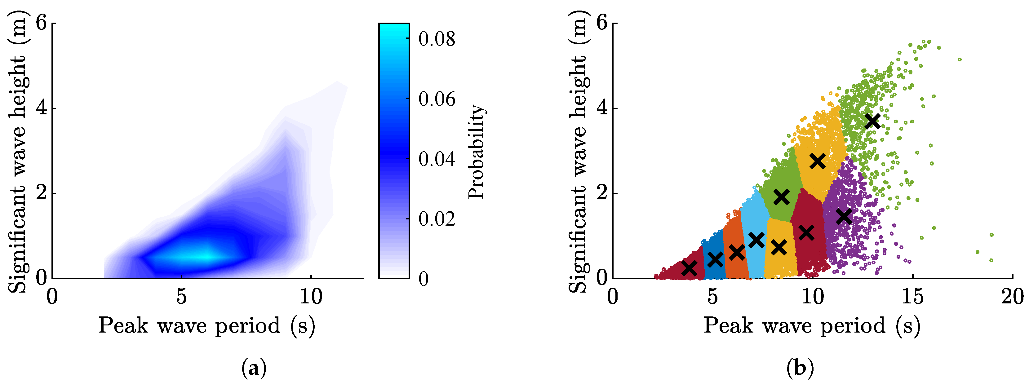
A wave energy converter chosen for this case study is a fully submerged cylindrical buoy connected to three tethers to absorb wave power from its motion in multiple degrees-of-freedom (or multiple modes). namely surge, heave and pitch. As shown in Figure 1, the geometry of this WEC is determined by the radius a and height H of the cylinder, tethers inclination angle α t , and the angle α a p that defines the tether attachment point (from the centre of mass of the buoy). The submergence depth (distance from the undisturbed water level to the top of the buoy) is considered fixed and equal to 2 m regardless of the buoy size. The mass of the buoy is taken as half the displaced mass of water m b = 0.5 ρ w V (the density of water is ρ w = 1025  kg/m 3 , and the buoy volume is V = π a 2 H ). The hollow buoy houses three direct mechanical drive power take-off units (each connected to the tether). Each PTO acts as a spring-damper system where stiffness and damping coefficients can be adjusted for each sea state.

2.2. Wave Climate

A potential wave energy development site located near the west coast of Marretimo Island (Italy) in the Mediterranean Sea is chosen for this analysis. According to the WXSD classification [20], this wave climate belongs to resource class 1 due to its low energy content (6.4 kW/m). The k-means clustering method has been applied to extract 10 sea states that represent this wave climate as shown in Figure 2 and listed in Table 1. A weighted aggregation of these 10 irregular sea states are used to calculate the annual average power production of the WEC. It is assumed that all waves are unidirectional and propagate in the positive x-direction.

2.3. Equations of Motion

The following time-domain model describes the WEC response under the wave and PTO loads:
M x ¨ ( t ) = F e x c ( t ) + F r a d ( t ) + F v i s c ( t ) + F b u o y ( t ) + F t e n s ( t ) ,
where the x R 6 × 1 is the buoy position vector in O x y z coordinate system, M is a mass matrix, F e x c is the wave excitation force, F r a d is the wave radiation force, F v i s c is the viscous drag force, F b u o y is the buoyancy force, F t e n s is the tether tension force expressed in the Cartesian space that includes the pre-tension force and control (PTO) forces. The force acting along the k-th tether can be modelled as Ft,k = F t 0 + K p t o Δ k + B p t o Δ ˙ k ( k = 1 3 ) being proportional to the tether extension Δ , the rate of change of the tether length Δ ˙ and includes the initial tension F t 0 . The PTO stiffness K p t o and damping B p t o coefficients take the same values for all three tethers. The transformation between the buoy velocity x ˙ and the tether velocity vector q ˙ = [ Δ ˙ 1 Δ ˙ 2 Δ ˙ 3 ] T has a form of q ˙ ( t ) = J 1 ( x ) x ˙ ( t ) , where J 1 ( x ) R 3 × 6 is the inverse kinematic Jacobian that depends on the buoy position at each time instance [34]. So the tether force vector can be converted to the Cartesian space according to F t e n s = J T F t .
The time-domain model in Equation (1) has a relatively high computation time and may not be suitable for optimisation purposes when a large number of evaluations are required. If to assume that all processes are Gaussian, it is possible to derive a spectral-domain model that can capture all required nonlinear forces using statistical linearisation technique [38,39]. The spectral-domain model approximates the system dynamics in the frequency domain by replacing all nonlinear terms with equivalent linear matrices [40]. The dynamic model in Equation (1) has two sources of nonlinearity: the viscous drag force Fvisc and the generalised tether tension force Ftens. Due to the fact that geometric nonlinearity contained within Ftens is much weaker than the quadratic nonlinearity in Fvisc, Ftens can be linearised around the zero position without loss of accuracy for the proposed configuration. If nonlinear effects from tethers become relevant, the equivalent terms can be derived as shown in [38,41,42]. Moreover, it should be noted that other nonlinear forces can be included in the model but omitted in this study, e.g., nonlinear Froude–Krylov force that becomes relevant when the buoy experiences large motion amplitudes [43]. As a result, a nonlinear dynamic Equation (1) is replaced by the equivalent frequency domain model:
[ ω 2 ( M + A ( ω ) ) + i ω ( B ( ω ) + B p t o + B e q ) + K p t o ] x ^ ( ω ) = F ^ e x c ( ω ) ,
where x ( t ) = R e { x ^   e i ω t } , the radiation force is expressed using the frequency dependent added mass A(ω) and radiation damping matrix B ( ω ) , F ^ r a d ( ω ) = ( ω 2 A ( ω ) + i ω B ( ω ) )   x ^ ( ω ) , the tether tension force is linearised as F ^ t e n s ( ω ) = ( i ω B p t o + K p t o ) x ^ ( ω ) (see [44] for more details), and the viscous drag force is replaced by F ^ v i s c ( ω ) = i ω B e q x ^ ( ω ) . The equivalent damping term Beq is unknown and determined iteratively (for each wave condition separately) using the procedure explained in [38]:
B e q = F v i s c x ˙ ,
where 〈·〉 indicates mathematical expectation, and the viscous force is interpreted as:
F v i s c = 1 2 ρ w C d A d ( | | x ˙ | | x ˙ ) ,
ρw is the density of water, Cd and Ad are the matrices of the drag coefficients and the cross-section areas of the buoy perpendicular to the direction of motion respectively, and ⊙ represents the Hadamard product (element-wise multiplication). Note that only the body velocity (not the relative fluid/body velocity) has been considered in the drag force formulation. A detailed methodology of how to incorporate the wave-particle velocity into the spectral-domain model is demonstrated in [45].
The following iterative procedure is used to estimate B e q and approximate the response of the WEC in irregular waves:
Step 1.
Define the sea state and corresponding incident wave spectrum S η ( ω ) .
Step 2.
Compute the power spectral density (PSD) matrix of the excitation force:
S F ( ω ) = S η ( ω ) f ^ e x c ( ω ) f ^ e x c * ( ω ) ,
where f ^ e x c is the vector of excitation force coefficients, and  ( ) * denotes the conjugate transpose of a vector/matrix.
Step 3.
Calculate the WEC response matrix assuming B e q = 0 6 × 6 in the first iteration:
H ( ω ) = [ ω 2 ( M + A ( ω ) ) + i ω ( B ( ω ) + B p t o + B e q ) + K p t o ] 1 .
Step 4.
Establish the power spectral density matrix of the buoy motion:
S x ( ω ) = H ( ω ) S F ( ω ) H * ( ω ) .
Step 5.
Calculate the covariance matrix of the WEC velocity:
σ x ˙ 2 = cov [ x ˙ , x ˙ ] = 0 ω 2 S x ( ω ) d ω .
Step 6.
Estimate the equivalent damping matrix B e q using the analytical expression from [38]:
B e q = F v i s c x ˙ = 1 2 8 π ρ w C d A d σ x ˙ 2 .
Step 7.
Check the convergence criteria:
| B e q [ n ] B e q [ n 1 ] | < δ .
where n corresponds to the iteration number, and the threshold is set to δ = 0.01 . If this condition is not satisfied, go to Step 3.
It can take up to 10 iterations to estimate Beq and the WEC response in irregular waves. Once calculated, the average power absorbed by each PTO unit k = 1 3 is calculated as [38]:
P ¯ k = B p t o σ q ˙ k 2 ,
where σ q ˙ k 2 is the variance of the tether length rate change q ˙ :
σ q ˙ k 2 = 0 ω 2 S q k ( ω ) d ω ,
and the transformation between the Cartesian coordinate system and the tether space is obtained using S q ( ω ) = J 0 1 S x ( ω ) J 0 T , where J 0 1 = J 1 ( x 0 ) is linearised about the nominal operating position x 0 = 0 6 × 1 .
The total power generated by three PTO units in an irregular wave with the significant wave height H s and peak wave period T p is:
P ¯ ( H s , T p ) = B p t o k = 1 3 σ q ˙ k 2 ( H s , T p ) .
The expected average annual power production from the WEC for a specific deployment site is estimated as:
P A A P = H s T p O ( H s , T p ) · P ¯ ( H s , T p ) ,
where the matrix O ( H s , T p ) contains the occurrence probability of each sea state within the wave climate.
To demonstrate that the spectral-domain model is an effective tool that can fully capture the nonlinear dynamics of the considered WEC while significantly decreasing the computation time, a comparison of average power estimated using three different models is shown in Figure 3. The frequency-domain model is implemented based on Equation (2) assuming Beq = 0, the spectral-domain model is specified in Equation (2) where Beq is estimated iteratively for each sea state, and the time-domain model is represented by Equation (1). Good agreement is achieved between the spectral-domain and time-domain models, while the frequency domain model significantly overestimates power generation potential of the WEC.

2.4. Economic Model

Levelised cost of energy (LCoE) is used to measure the economic attractiveness of the proposed energy project. Due to the lack of publicly available information of the detailed cost estimations for wave energy technology, [46] proposed to approximate LCoE by the following equation:
LCOE ( kWh ) = RDC × ( Energy ( MWh ) Mass ( kg ) ) 0.5 ,
where RDC is a site-specific coefficient that is set to 1 in this study, the characteristic mass of the system includes the mass of the buoy and the anchoring system.
The characteristic mass of the WEC is calculated using the following assumptions:
-
The mass of the buoy is calculated based on a given geometry as m b = 0.5 ρ w π a 2 H ;
-
The needed mass of the anchoring system (three piles) relays on the tether tension associated with buoyancy and the wave force, and can be approximated by m a s 0.116 F t p e a k using case presented in [47] as a reference. The tether peak force ( 99 % = 2.57 σ F t ) is estimated from the spectral-domain model.
As a consequence, the LCoE model applied in this research is:
LCOE = ( 8760 P A A P m b + m a s ) 0.5 .

2.5. Implementation

To estimate the power output and LCoE for any WEC geometry, Equation (2) is solved inMATLAB. The mass matrix has a diagonal form M = diag(mb, mb, mb, Ixx, Iyy, Izz) with moments of inertia calculated for the cylindrical body. Hydrodynamic parameters of the WEC, including the added mass A(ω), hydrodynamic damping B(ω), and excitation force vector F ^ e x c ( ω ) are estimated using a semi-analytical model [48,49]. Beq is calculated based on the iterative procedure explained in Section 2.3.
Even though only one geometric shape (vertical cylinder) is used in the study, the magnitude of the viscous drag force, and the corresponding Beq, are highly dependent of the ratio between the cylinder height to its diameter, especially for the heave mode. Therefore, it order to develop an optimisation procedure that can accommodate WEC geometries with various aspect ratios ( H / a ), the drag coefficient in heave is expressed as a function C d 3 = 0.12 ( H / a ) + 1.2 based on published data [50] shown in Figure 4. Drag coefficients in other directions are not sensitive to the cylinder aspect ratio and are kept fixed C d 1 = C d 2 = 1 for surge and sway, and  C d 4 = C d 5 = 0.2 for roll and pitch. The irregular waves from Table 1 are modelled using the Bretschneider (modified Pierson–Moskowitz) spectrum according to [51].

3. Optimisation Configuration Models

In this research, The optimisation decision variables of the cylinder are including the radius of the buoy a, the aspect ratio that is considered as the proportion of the height over the radius of the buoy ( H / a ), two tether angles (attachment α a p and inclination angle α t ), two vectors of power take-off parameters, damping and stiffness coefficients represented b p t o = [ B p t o ( 1 ) , B p t o ( 2 ) , , B p t o ( N ) ] T and k p t o = [ K p t o ( 1 ) , K p t o ( 2 ) , , K p t o ( N ) ] T , respectively. The length of each PTO vector is N = 10 . The whole number of decision designs are 24 which should be optimised in the following:
z 1 = [ a , H , α t , α a p , k p t o R N × 1 , b p t o R N × 1 ] .
z 2 = [ a , ( H / a ) , α t , α a p , k p t o R N × 1 , b p t o R N × 1 ] .
We apply two fitness functions in order to maximise the power output and minimise the LCoE.
(i)
The average annual produce power output computed utilising Equation (14), that is maximised as
f O 1 = arg max z P A A P ( z ) , subject to : z 1 [ z min , z max ]
(ii)
The LCoE is minimised using the below equation that is specified in Equation (16):
f O 2 = arg min z LCOE ( z ) , subject to : z 2 [ z min , z max ]
Table 2 shows the ranges of all design variables which are involved in the optimisation process.

4. Optimisation Algorithms

In this paper, we focus on two widespread optimisation strategies in order to maximise harnessed power and minimise the levelised cost of energy (LCoE) of a fully-submerged three-tether WEC. The first approach applies optimisation algorithms to all decision variables simultaneously. These design variables consist of the buoy geometry parameters (radius a, height H and aspect ratio ( H / a )), the tether angles (inclination angle α t and the tether attachment angle α a p ), and the PTO parameters (spring stiffness k p t o and damping coefficients k p t o ). In total, there are 24 parameters that are optimised all-at-once.
The second strategy is to apply bi-level optimisation methods [52], which solve the problem using a two-level optimisation procedure, where one optimisation problem is nested within the other. The outer optimisation task is generally regarded as the upper-level optimisation problem, and the interior one is recognised as the lower-level optimisation problem. A significant characteristic of the bi-level optimisation problem is that the fitness functions of each level may be partly defined by variables advised by other levels. Following this strategy, we propose two bi-level optimisation methods and compare their performance with seven other well-known global search methods. The details of the optimisation algorithms performed for each strategy are outlined in Table 3.

4.1. All-at-Once Optimisation

Various factors associated with WEC design, tether angles and PTO parameters combined to form a non-convex, dynamic, constrained and large-scale optimisation problem. These challenges serve as our primary motivation for applying the meta-heuristics like evolutionary and swarm optimisation algorithms. We apply and compare the performance of seven well-known meta-heuristics that reliably optimise all decision variables of WECs all-at-once. This optimisation process leads to maximise the produced power and minimise the levelised cost of energy. The optimisation methods applied in this research include 1+1EA [59]; Differential Evolution (DE) [57], Covariance matrix adaptation evolution strategy (CMA-ES) [55], Particle Swarm Optimisation (PSO) [56], Grey Wolf Optimiser (GWO) [35] and two state-of-the-art self-adaptive optimisation methods including SaDE [58] and LSHADE-EpSin [36].

4.1.1. L-SHADE with an Ensemble Pool of Sinusoidal Parameter Adaptation (LSHADE-EpSin)

The Differential Evolution (DE) algorithm, and its adaptive and self-adaptive variants, are simple and robust evolutionary algorithms. Researchers from various fields of science and engineering have applied DE algorithms to various optimisation problems, notwithstanding problems with characteristic such being continuous, multi-modal, combinatorial or mixed variable. DE is able to obtain superior optimisation results across widely encountered real-world engineering problems [60,61]. Among a wide range of self-adaptive DE algorithms, LSHADE-EpSin performs outstandingly in solving different benchmarks and real-world problems [36]. LSHADE-EpSin is a modified version of the L-SHADE algorithm [62] with linear population size reduction and an ensemble pool of sinusoidal parameter adaptations. L-SHADE is a developed version of the SHADE algorithm [63] that practices a history-based parameter adaptation trajectory based on the JADE algorithm [64] which proposed the novel mutation strategy (current/to/pbest).

Mutation Strategy with External Archive

In LSHADE-EpSin, one of the best-performing mutation strategies for generating promising mutant vectors during the optimisation process is current-to-pbest/1 which is initially proposed by JADE. This mutation strategy can be seen in Equation (21).
v i , g = x i , g + F i , g ( x p b e s t , g x i , g ) + F i , g ( x r 1 , g x r 2 , g )
where x p b e s t , g is chosen from the best solutions N × p ( p [ 0 , 1 ] ) of the current parent population (g). x r 1 , g is randomly taken from the population and x r 2 , g is randomly chosen from a combination of the current population and the external archive (A). The external archive keeps a record of the lower-ranking parents recently replaced by offspring.

Ensemble of Parameter Adaptation

An ensemble of parameter configurations is used in LSHADE-EpSin to control the adaptation of parameters. The adaptive parameters are associated with a combination of two sinusoidal formulas to adjust the scaling factor. Firstly, a non-adaptive sinusoidal adjustment technique is used to adjust the scale factor ( F i , g ) which decreases during the optimisation process. Equation (22) shows this non-adaptive technique.
F i , g = 1 2 × ( s i n ( 2 π × f r e q × g s 1 + π ) × i t e r m a x g s 1 i t e r m a x + 1 )
where f r e q describes a pre-defined frequency for the sinusoidal function and i t e r denotes the current generation number ( g s 1 < = i t e r m a x 2 ). The second strategy for the adjustment of the scale factor is an adaptive sinusoidal adjustment method. This formulation can be seen in Equation (23).
F i , g = 1 2 × ( s i n ( 2 π × f r e q × g s 1 ) × g s 1 i t e r m a x + 1 )
where f r e q is an adaptive frequency based on a Cauchy distribution and a successful history-based of settings. i t e r denotes the current generation number. One of the most effective DE parameter adaptation techniques is recording an archive of both mutation factors and probabilities of crossover based on their success during the optimisation process. The control parameters history-based was proposed by Zhang et al. [64] in JADE. In each generation of JADE, in order to generate an offspring, we have an array of the crossover probability rate that is produced based on a normal distribution of the mean μCR and variance at 0.1. The successful crossover probabilities SCR are recorded and updated at each generation. The μCR is initialised by 0.5 and in the next generation it is updated by Equation (24).
μ C R = ( 1 c ) × μ C R + c × m e a n A ( S C R )
where c is a constant generated between 0 and 1 randomly and meanA is a simple arithmetic mean. Likewise, the mutation factor Fi of each xi is separately generated at each generation, as stated in a Cauchy distribution with the mean μF and scale parameter 0.1. (Equation (25))
F i = r a n d c i ( μ F ,   0.1 )
where the r a n d c i is the Cauchy distribution. All successful mutation factors are archived and point out as a set of SF at the end of each generation. The value of μF is updated using Equation (26).
μ F = ( 1 c ) × + c × m e a n L ( S F )
where meanL is the Lehmer mean [65] and computed as follows:
m e a n L ( S F ) = F S F F 2 F S F F
Linear Population Size Reduction
The LSHADE-EpSin algorithm benefits from a linear reduction in population size to fit the population size (N) iteratively at each generation as exposed in the following equation:
N g + 1 = R o u n d [ ( N m i n N m a x i t e r m a x ) × i t e r + N m a x ]
where Nmin is the minimum population size, and initialised at 4 that is required to make the current-to-pbest mutation strategy. The four required solutions are x i , x b e s t p , x r 1 and x r 2 . The mutant vector of this strategy is generated using Equation (29).
V i , g = x i , g + F i × ( x b e s t , g p x i , g ) + F i ( x r 1 , g x r 2 , g )

Local Search

In order to extend the exploitation capability of LSHADE-EpSin, a stochastic local search i s proposed that works based on Gaussian Walks. The local search is activated when the population size is less than 20 ( N i n i = 25 ), and 25 random samples are evaluated to exploit the neighbourhood of the best-found design among the current population. The Gaussian walks applied can be seen in Equation (30).
y i = N ( μ b , σ ) + ( r 1 × x b e s t r 2 × x i )
where x b e s t is the best-found solution in the local search and μ b is equal to x b e s t . r 1 and r 2 are two uniform random numbers from the range of [ 0 , 1 ] . Besides, the standard deviation ( σ ) of this Gaussian Walks is calculated using Equation (31).
σ = l o g ( i t e r ) i t e r × ( x i x b e s t )

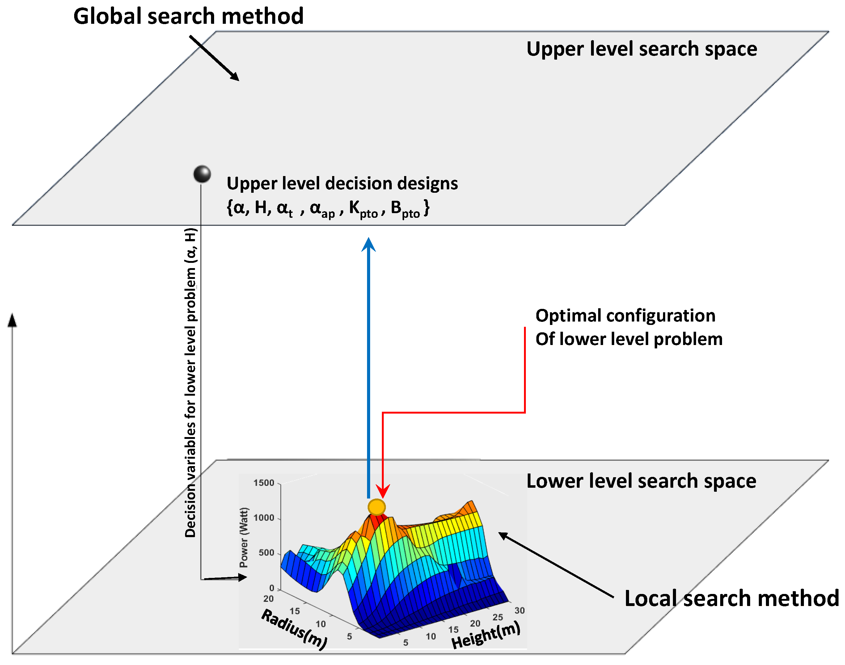
4.2. Bi-Level Optimisation

In this paper, we propose two bi-level optimisation methods, including Bi-level-1 (SaDE+NM) and Bi-level-2 (LSHADE-EpSin+NM). We also provide a general formulation in order to maximise the harnessed power and minimise the LCoE of a cylindrical wave energy converter. These proposed approaches comprise two levels of optimisation tasks where one optimisation process is nested within the other. The exterior optimisation method (which is a global search method) is referred to as the leader’s (upper level) optimisation process. In the upper level, we apply two self-adaptive meta-heuristics, including Self-adaptive DE (SaDE) and LSHADE-EpSin. Both methods improve the ability of an adaptive learning strategy to fine-tune the control parameters and mutation strategy and demonstrate a considerable performance in optimising real engineering problems [66,67].
In the second level, the internal method is recognised as the follower’s (lower level) optimisation process. In the current study, the inner method is a Nelder–Mead (NM) simplex search method [68]. NM simplex is a downhill local search method, and it is straightforward to hybridise combine with other meta-heuristic methods. The primary reason for such hybridisation (or for using NM as the lower-level in a bi-level method) is to tune a more suitable trade-off between global optimality and computational budgets [69,70].
Figure 5 shows that the proposed bi-level optimisation framework consists of a global search method designed to optimise all decision variables in the upper-level, and both geometry parameters (radius and height) that given from upper-level decision vector are optimising in the lower-level. To adjust the geometry parameters of the cylinder, we use a local search method. The best-found geometry configuration in the lower-level will be replaced in the upper-level decision variables.
The pseudo-code of the proposed Bi-level-2 algorithm is shown in Algorithm 1. It can be seen that the algorithm is divided into two primary sections. At the top level, we have a self-adaptive DE (LSHADE-EpSin) employing two strategies to adjust the control parameters. These strategies are (1) adaptive sinusoidal increasing adjustment and (2) non-adaptive sinusoidal decreasing adjustment. The benefit of this ensemble approach is that it allows the algorithm to converge to a sufficient balance [36] between searching the neighbourhood of current bet-found solutions and the exploration of non-visited search space zones. In the lower-level, there are two nested inner local search methods. The initial local search is used to explore the search space of the cylinder dimensions (radius and height) where other decision variables are fixed. Next, both tether angles (inclination and attachment) are optimised using the second local search. In order to save computational budget, we define a performance criterion for both local search methods. This condition evaluates the local search performance; if the obtained power improvement cannot satisfy the criterion, Bi-level-2 will withdraw the local optimisation process and allocate the remaining budget to the global search method.

Tuning the Local Search

One of the significant parameters of the bi-level optimisation method is the maximum evaluation number ( M a x e v a l ) of the local search (NM). Tuning this variable plays an important role in obtaining a greater balance between saving on the computational budget and converging to the local optimum as much as possible. In order to tune the M a x e v a l , we perform the local search to optimise the WEC geometry parameters ( a , H ) and keep the other decision variables fixed. This experiment iterates ten times with different initial solutions. Meanwhile, the same tuning process runs to optimise both tether angles. Figure 6 shows the convergence curves of these experiments. We observe that the local search converges rapidly to a local optimum in the geometry and tether angles optimisation processes after 20 and 40 iterations, respectively on average. Therefore, we set the M a x e v a l of the local search to 20 and 40 iterations.

5. Optimisation Results and Discussions

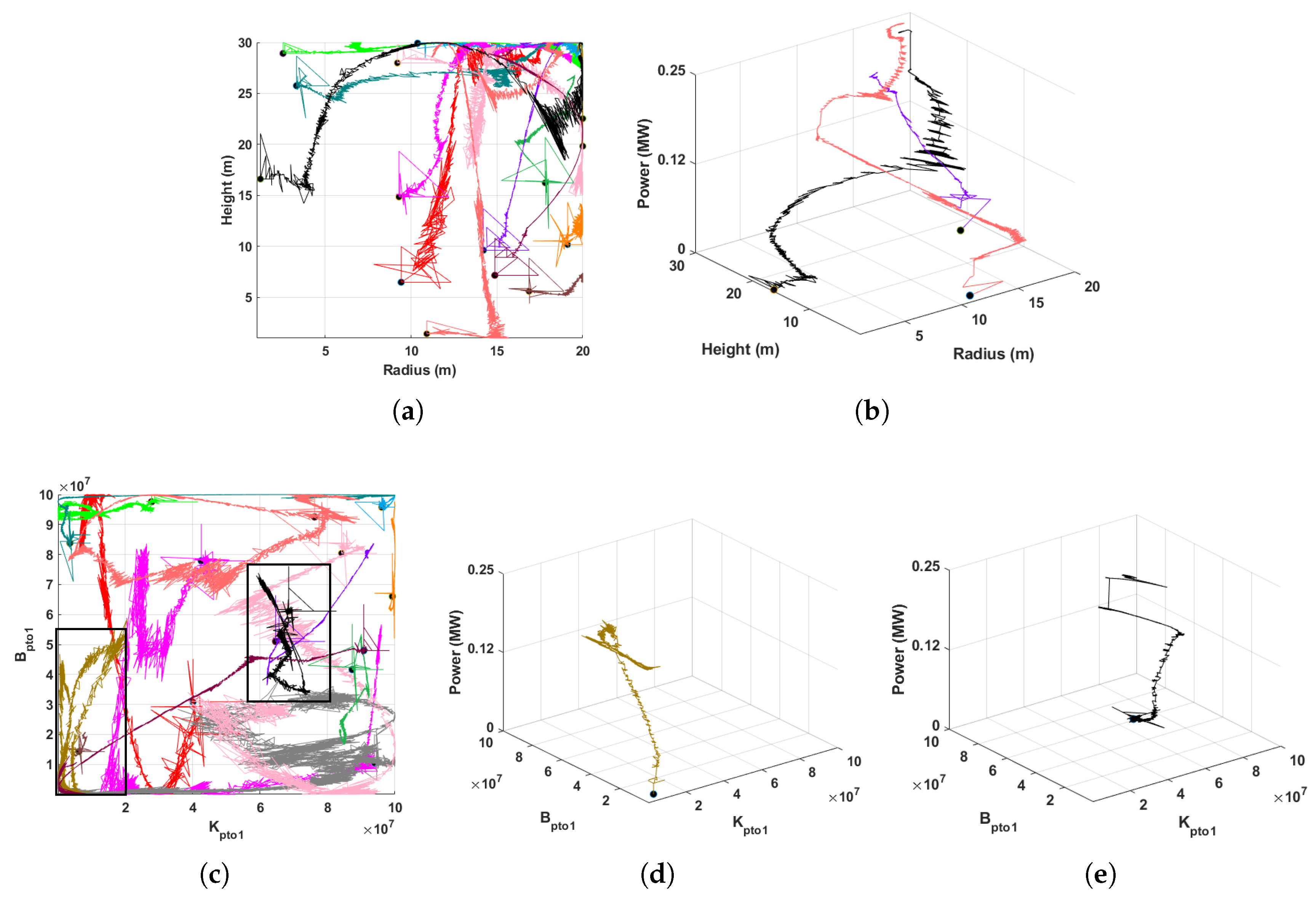
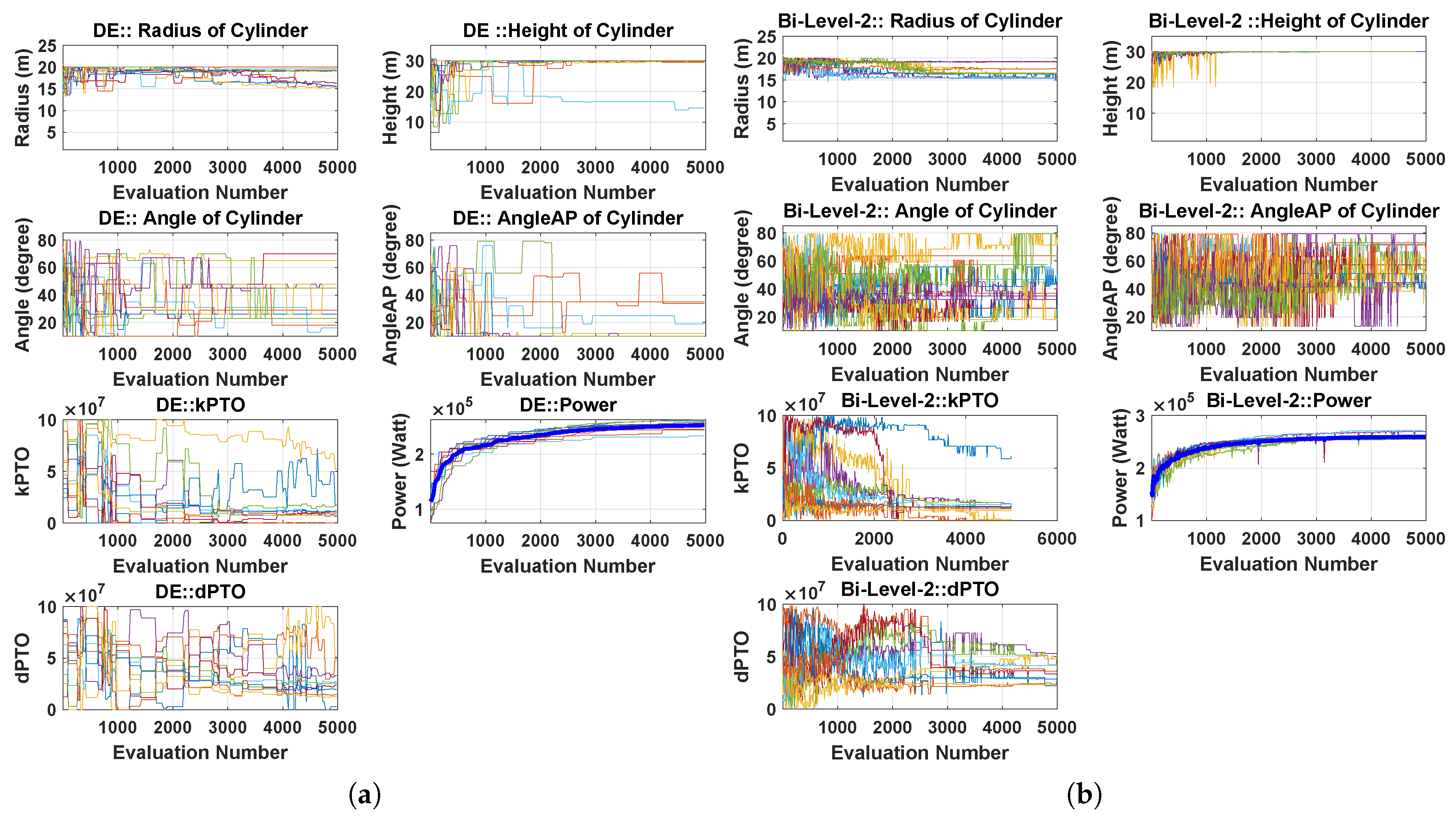
5.1. Multi-Modality of Search Space

In order to characterise the search space, we perform an experiment using a Nelder–Mead (NM) search method. Twenty random initial configurations are generated and NM is applied to optimise the absorbed power output. Figure 7 shows the trajectory of the NM performance during the optimisation process. It can be seen that the majority of the trajectories in the cylinder dimension (subplot (a)) converged to a specific area of the search space as expected. This is because large WECs can harness more power than small ones. The second observation is that the PTO search space is not uni-modal and each trajectory converged to different configurations (subfigure (c,d,e)).

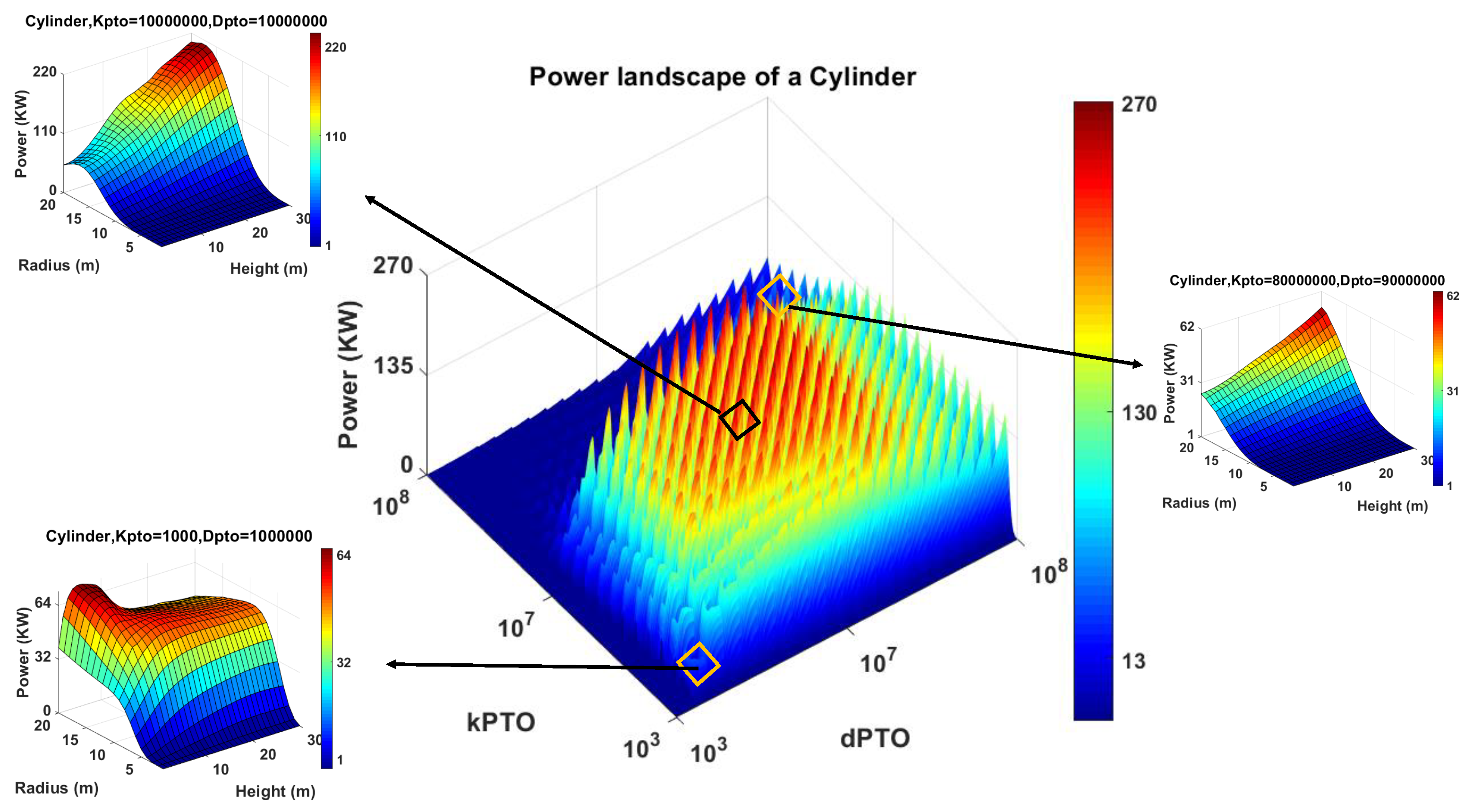
5.2. Power Landscape Analysis

With regard to evaluating the impact of each buoy design variable on the level of produced power, we perform a sensitivity analysis experiment. Here, we assume both tether angles are kept fixed at 45°; note that this size is not optimal, because tether angles should be adjusted based on the buoy’s dimensions, as recommended by prior works [34]. Moreover, the search space of the K p t o and B p t o parameters are discretised, where each interval is 10 6 . In the next step, for each discrete configuration of PTO parameters, we evaluate the importance of the cylinder dimensions ( a , H ) using a grid search technique where the discretisation step size is 1 (m).
The results are shown in Figure 8, which includes 400 sub-figures. Each sub-figure represents the relationship of the cylinder radius and height sizes with the absorbed power, where the K p t o and B p t o are fixed. It is important to note that a variation in the size of the radius has a more substantial effect on the power output than a variation in the cylinder height. In this wide power landscape, we can see that the maximum produced powers are achieved when the PTO parameters are assigned around 10 7 , and the buoy radius and height sizes are large. However, it should be noted that the effect of PTO parameters on the absorbed power is more significant than the size of the cylinder dimensions.
Algorithm 1 Bi-level Optimisation method (LSHADE-EpSin+NM)
procedureBi-level Optimisation method
 Initialization
    P = { a 1 , H 1 , α t 1 , α a p 1 , K 1 1 , . . . , K 1 10 , B 1 1 , . . . , B 1 10 ,
    , a N , H N , α t N , α a p N , K N 1 , . . . , K N 10 , B N 1 , . . . , B N 10 } ▹ initial population
   M: μ F = μ CR=0.5▹ initialise memory of first control settings
   M f r e q : μ freq = 0.5, I m p r a t e d = I m p r a t e α = 1 ▹ initialise memory of second control settings
 Upper-Level (Global search method)
   for i t e r in i t e r m a x do▹ termination criteria
    if i t e r > i t e r m a x 2 then
     Call second control parameter settings
      S F = S C R = ▹ Reset successful mean vectors
      r i = r a n d ( 1 , H ) ▹ Generate a random index, H is memory size
      F i = r a n d c ( μ F r i , 0.1 ) , C R i = r a n d n ( μ C R r i , 0.1 )
    end if
    if i t e r i t e r m a x 2 then
     Call first control parameter settings
      c = r a n d ( 0 , 1 )
     if c < 0.5 then
       F i = 1 2 × ( s i n ( 2 π × f r e q × i t e r + π ) × i t e r m a x i t e r i t e r m a x + 1 )
     else
       F i = 1 2 × ( s i n ( 2 π × f r e q × i t e r ) × i t e r i t e r m a x + 1 )
     end if
     Generate C R i same as first control parameters (Equation 23)
    end if
    for i = 1 to N do
     Generate p = r a n d ( 0 , 1 ) × n , n = 0.1 × N
      v i = x i + F i × ( x p b e s t x i ) + F i × ( x r 1 x r 2 ) ▹ Mutation c u r r e n t - t o - p b e s t / 1
      u i , iter j = { v i , iter j , if ( rand < CR i ) or ( j = = j r a n d ) P i , i t e r j , Otherwise ▹ Binomial Crossover
      P i , iter + 1 = { u i , iter , if ( f ( u i , iter ) > f ( P i , iter ) ) M a x i m i s a t i o n P i , i t e r , Otherwise ▹ Selection
     Store successful F i and C R i
    end for
    Update the memory according to used settings
    Update the population size by Equation (28)
     N d i f f = N g N g + 1
    Sort P i t e r based on the fitness function
    Remove worst solutions N d i f f from P i t e r AND Select the best solution P b e s t
Lower-Level (Local search method)
    if I m p r a t e d > 0.001% then▹ Optimise Cylinder dimension
      P b e s t ( a , H ) = N e l d e r M e a d ( P b e s t ( a , H ) , M a x e v a l )
     Compute improvement rate I m p r a t e d
    end if
    if I m p r a t e α > 0.001% then▹ Optimise tether angles
      P b e s t ( α t , α a p ) = N e l d e r M e a d ( P b e s t ( α t , α a p ) , M a x e v a l )
     Compute improvement rate I m p r a t e α
    end if
    Update P i t e r b e s t by the best-found NM configurations
   end for
end procedure

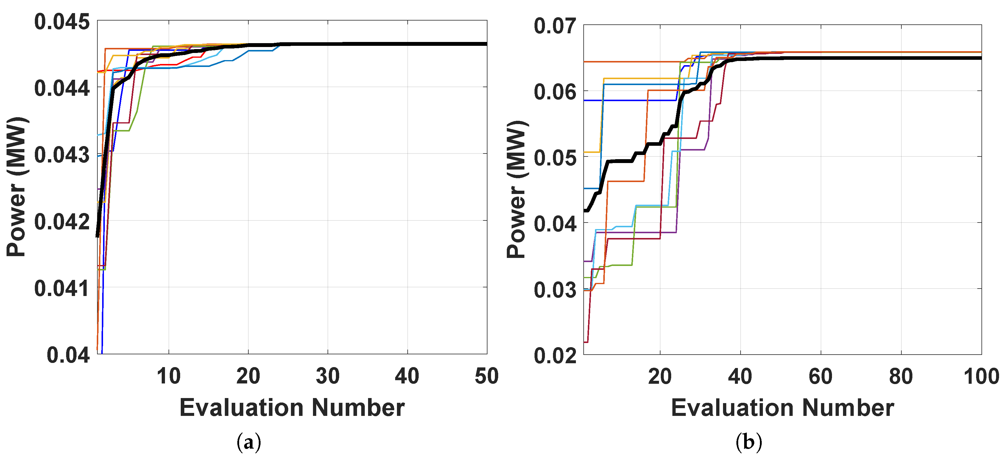
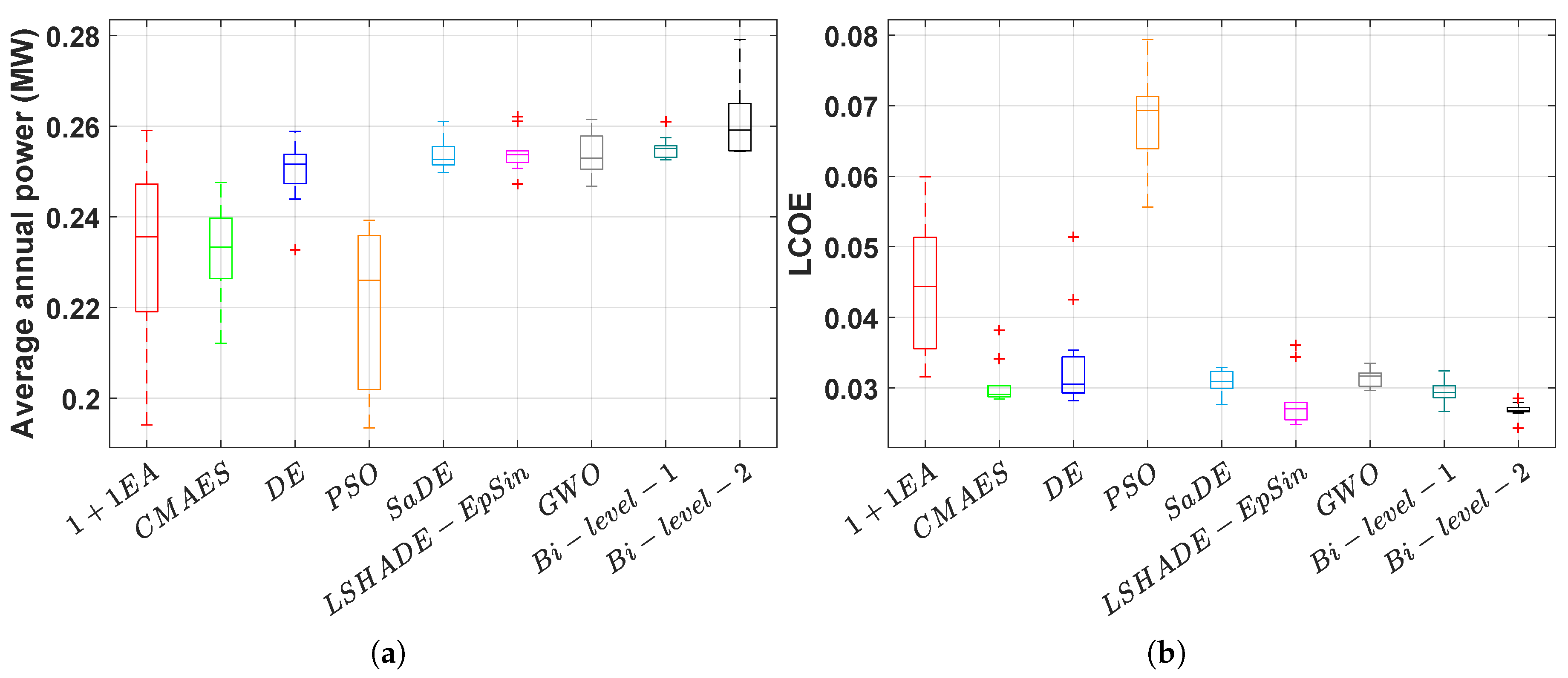
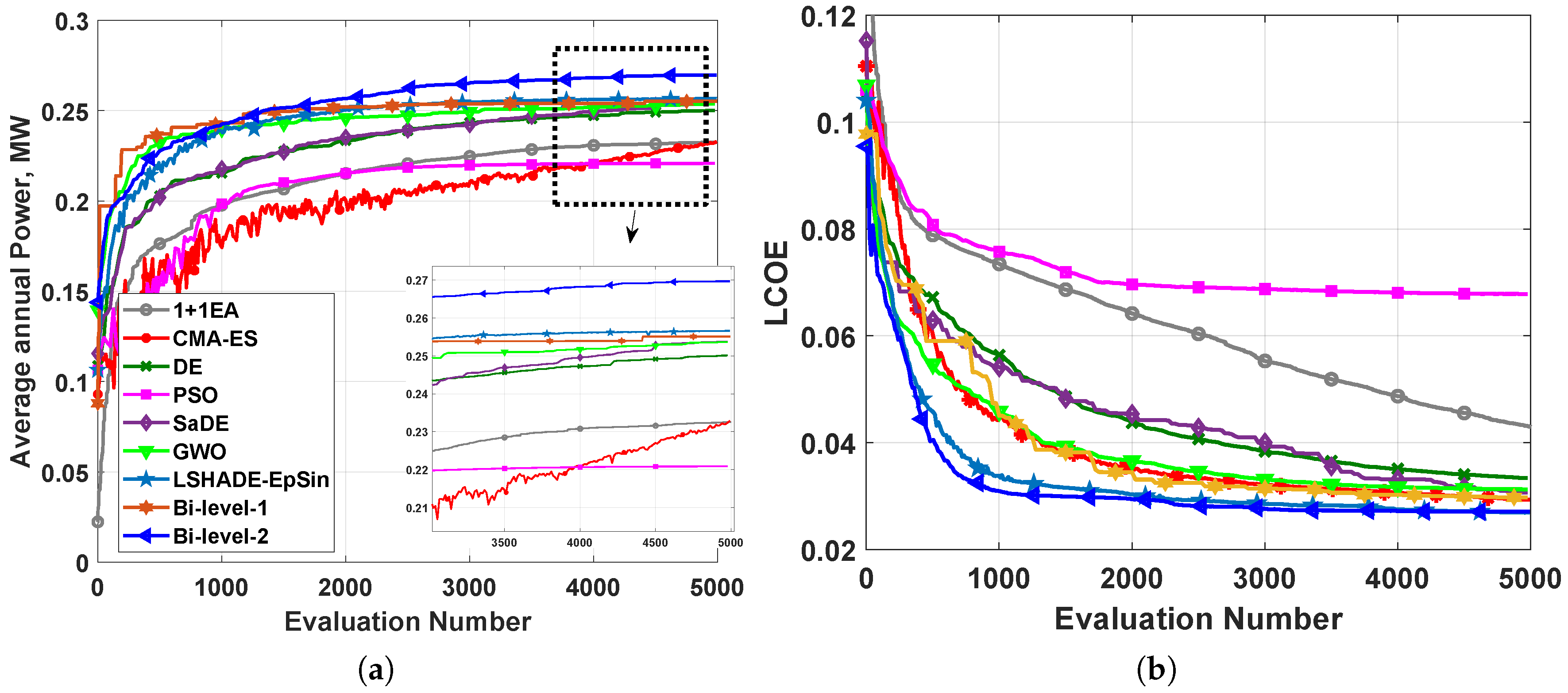
5.3. The Annual Average Power Output Maximisation

In this section, we describe the optimisation results of our cylinder design experiments in order to maximise the annual average power output. Furthermore, we compare the performance of the optimisation algorithms outlined above in terms of best-found designs and speed of convergence.
Table 4 reports the best-found cylinder designs using seven meta-heuristics and two new bi-level optimisation methods that produced the highest power output among all ten runs. Furthermore, it can be seen that Bi-level-2 performs better than other applied optimisation methods and that it can produce a considerable amount of power of 279 kW. The second observation is that almost all (8 out of 9) optimisation methods converged to the cylinder of 15 m radius with the largest possible height of 30 m. However, it should be noted that producing electricity using such large WECs can be expensive, due to the high manufacturing costs. In terms of the angles and PTO settings, a large range of values is proposed by all optimisation methods even though the maximised power output is not dramatically different. This fact proves that it is not straightforward to optimise a multi-mode WEC due to the strong dependencies between angles, PTO parameters, and the hydrodynamic model which dominates the power absorption (heave, surge or pitch).
Table 5 presents the average best-found power output per each run for all optimisation methods. Bi-level-2 is not only capable of finding the best design configuration; it also performs the best average power output (Figure 9a) compared with other meta-heuristics. In terms of the convergence rate, Figure 10a depicts the applied optimisation method experiments during the 5000 evaluations. As we can see, GWO and LSHADE-SeSin rapidly converge to considerable settings; however, they could not sustain this upward trajectory and converge near locally optimal designs. Obviously, the fastest convergence rate is allocated to Bi-level-2.

5.4. LCoE Minimisation

In this section, we describe the second applied objective function related to LCoE and approximated as a ratio of the generated energy to the significant mass of the system. The best-found LCoE values and their relevant cylinder configurations which are obtained using nine meta-heuristic approaches are shown in Table 6. Interestingly, all optimisation methods (except PSO) converged to a narrow range of radii between 5 and 7.3 m, with the smallest possible aspect ratio of 0.4. This geometry leads to the fact that the power generation will be dominated by the heave mode rather than surge. Moreover, this is clearly seen from the optimised values of the tether angles as to absorb power from the vertical motion, the tether angles should be closer to vertical leading to αt < 35 °. Another important finding is that the power production of WECs optimised for LCoE is relatively low leading to 28.3 kW.
Figure 9b shows the box-and-whiskers plot for the best configurations of the WEC which deliver the minimum LCoE for each run for nine search heuristics. It can be seen that the performance of Bi-level-2 is more reliable than that of the other meta-heuristic algorithms we applied. Both LSHADE-EpSin and Bi-level-1 show the next best average performances by 0.028 and 0.0295, respectively.
Investigating the convergence trajectories (Figure 10) from this experiment in the real wave model, it is clear that Bi-level-2 converges faster than other optimisation methods. It is noteworthy that among the seven optimisation methods in the all-at-once strategy, the LSHADE-EpSin convergence speed is substantially better than the others due to both adaptive and non-adaptive strategies in order to adjust the control parameters as well as to conduct an embedded local search in the initial iterations. However, it can be seen that the convergence rate of GWO is considerable in the initial 1000 evaluations.
In order to see the convergence performance of Bi-level optimisation algorithms, the search trajectory of the best agent in each generation for all decision variables is shown in Figure 11. Initially, we can see the high convergence ability of Bi-level-2 compared with DE in order to find and converge to the optimal range of both radius and height. Meanwhile, It can be observed that Bi-level-2 tends to explore promising areas of the tether angle search space broadly, and finally, to exploit the best values.

6. Conclusions

In this paper, two new bi-level optimisation methods are proposed with the aim of maximising the harnessed power output. These methods are also designed to minimise the levelised cost of energy of a fully-submerged, cylindrical WEC with three tethers for the wave climate of a Mediterranean sea site in the west of Sicily, Italy (featuring unidirectional irregular waves). The optimisation of a combination of WEC radius, height, tether inclination and attachment angles, and power take-off parameters is a relatively computationally expensive (5000 evaluations take around 15 h), multi-modal, large-scale and complex problem. These characteristics provided the principal motivation for investigating and proposing a faster and more reliable optimisation technique. With this in mind, we applied a bi-level strategy to optimise the design variables at various levels. A global search method was used at the upper level to optimise the parameters of the whole WEC’s. Furthermore, in the lower level, a Nelder–Mead (NM) simplex search method was applied to adjust the geometry settings and tether angles. To systematically compare the effectiveness of the proposed optimisation method, we considered seven state-of-the-art evolutionary and swarm algorithms. The experimental results showed that the bi-level method can outperform other meta-heuristics in terms of both convergence rate and the quality of WEC’s configuration. Moreover, according to the best-found configurations, if we focus on maximising the harnessed power output without considering the costs, a large cylindrical buoy is recommended. However, the cheapest energy can be delivered by a relatively small WEC with a radius of 5 m and a height of 2 m.

Author Contributions

Conceptualization, M.N., N.Y.S., B.A. and M.W.; Data curation, N.Y.S. and M.M.N.; Formal analysis, M.N. and N.Y.S.; Methodology, M.N., N.Y.S., M.M.N., E.A., B.A. and M.W.; Resources, M.M.N.; Validation, M.N. and N.Y.S.; Visualization, M.N., N.Y.S., B.A. and M.W.; Writing—original draft, M.N., N.Y.S. and M.M.N.; Writing—review and editing M.N., N.Y.S., D.A.G., B.A. and M.W.; Supervision, D.A.G., B.A. and M.W.; project administration, M.W. All authors have read and agreed to the published version of the manuscript.

Funding

This research was funded by European Union’s Horizon 2020 research and innovation programme under grant agreement No 727277 within the project ODYSSEA “Operating a network of integrated observatory systems in the Mediterranean sea” in order to collect data.

Acknowledgments

The authors would like to express their gratitude to Civil Engineering Department of Catania University and Favignana Municipality for their cooperation to provide all data. This research has been carried out within ODYSSEA project that received funding from the European Union’s Horizon 2020 research and innovation programme under grant agreement No 727277. Moreover, we would like to show our gratitude to Fabien Voisin from the information technology and digital services, the University of Adelaide due to his valuable participation in the parallel computing services. This research is supported by the supercomputing resources provided by the Phoenix HPC service at the University of Adelaide.

Conflicts of Interest

The authors declare no conflict of interest.

Abbreviations

The following abbreviations are used in this manuscript:
WECWave Energy Converter
PTOPower Take-off system
PSOParticle Swarm Optimisation
DEDifferential Evolution
SaDESelf adaptive Differential Evolution
CMA-ESCovariance Matrix Adaptation Evolution Strategy
LSHADELocal Success-history Adaptive Differential Evolution

References

  1. Murdock, H.E.; Gibb, D.; André, T.; Appavou, F.; Brown, A.; Epp, B.; Kondev, B.; McCrone, A.; Musolino, E.; Ranalder, L.; et al. Renewables 2019 Global Status Report; United Nations Environment Programme: Nairobi, Republic of Kenya, 2019; Available online: http://hdl.handle.net/20.500.11822/28496 (accessed on 19 September 2020).
  2. Tronchin, L.; Manfren, M.; Nastasi, B. Energy analytics for supporting built environment decarbonisation. Energy Procedia 2019, 157, 1486–1493. [Google Scholar] [CrossRef]
  3. Mazzoni, S.; Ooi, S.; Nastasi, B.; Romagnoli, A. Energy storage technologies as techno-economic parameters for master-planning and optimal dispatch in smart multi energy systems. Appl. Energy 2019, 254, 113682. [Google Scholar] [CrossRef]
  4. Aderinto, T.; Li, H. Ocean wave energy converters: Status and challenges. Energies 2018, 11, 1250. [Google Scholar] [CrossRef] [Green Version]
  5. Falnes, J. A review of wave-energy extraction. Mar. Struct. 2007, 20, 185–201. [Google Scholar] [CrossRef]
  6. Astariz, S.; Iglesias, G. Wave energy vs. other energy sources: A reassessment of the economics. Int. J. Green Energy 2016, 13, 747–755. [Google Scholar] [CrossRef]
  7. Wen, Y.; Wang, W.; Liu, H.; Mao, L.; Mi, H.; Wang, W.; Zhang, G. A Shape Optimization Method of a Specified Point Absorber Wave Energy Converter for the South China Sea. Energies 2018, 11, 2645. [Google Scholar] [CrossRef] [Green Version]
  8. Alamian, R.; Shafaghat, R.; Safaei, M.R. Multi-Objective Optimization of a Pitch Point Absorber Wave Energy Converter. Water 2019, 11, 969. [Google Scholar] [CrossRef] [Green Version]
  9. Esmaeilzadeh, S.; Alam, M.R. Shape optimization of wave energy converters for broadband directional incident waves. Ocean Eng. 2019, 174, 186–200. [Google Scholar] [CrossRef] [Green Version]
  10. Wang, L.; Ringwood, J.V. Geometric optimization of a hinge-barge wave energy converter. In Proceedings of the 13th European Wave and Tidal Energy Conference, Napoli, Italy, 1–6 September 2019; p. 1389. [Google Scholar]
  11. Garcia-Teruel, A.; Forehand, D.I.M.; Jeffrey, H. Metrics for wave energy converter hull geometry optimisation. In Proceedings of the 13th European Wave and Tidal Energy Conference EWTEC, Napoli, Italy, 1–6 September 2019. [Google Scholar]
  12. Sergiienko, N.Y.; Neshat, M.; da Silva, L.S.; Alexander, B.; Wagner, M. Design optimisation of a multi-mode wave energy converter. In Proceedings of the ASME 2020 39th International Conference on Ocean, Offshore and Arctic Engineering (OMAE2020), Fort Lauderdale, FL, USA, 28 June–3 July 2020. [Google Scholar]
  13. Abdelkhalik, O.; Zou, S.; Robinett, R.D.; Bacelli, G.; Wilson, D.; Coe, R.G.; Korde, U.A. Multiresonant Feedback Control of a Three-Degree-of-Freedom Wave Energy Converter. IEEE Trans. Sustain. Energy 2017, 8, 1518–1527. [Google Scholar] [CrossRef]
  14. Neshat, M.; Alexander, B.; Sergiienko, N.; Wagner, M. A Hybrid Evolutionary Algorithm Framework for Optimising Power Take Off and Placements of Wave Energy Converters. arXiv 2019, arXiv:1904.07043. [Google Scholar]
  15. Sharp, C.; DuPont, B. Wave energy converter array optimization: A genetic algorithm approach and minimum separation distance study. Ocean Eng. 2018, 163, 148–156. [Google Scholar] [CrossRef]
  16. Fang, H.W.; Feng, Y.Z.; Li, G.P. Optimization of Wave Energy Converter Arrays by an Improved Differential Evolution Algorithm. Energies 2018, 11, 3522. [Google Scholar] [CrossRef] [Green Version]
  17. Neshat, M.; Alexander, B.; Wagner, M.; Xia, Y. A detailed comparison of meta-heuristic methods for optimising wave energy converter placements. In Proceedings of the Genetic and Evolutionary Computation Conference. ACM, Kyoto, Japan, 15–19 July 2018; pp. 1318–1325. [Google Scholar]
  18. Neshat, M.; Alexander, B.; Sergiienko, N.Y.; Wagner, M. Optimisation of Large Wave Farms Using a Multi-Strategy Evolutionary Framework. In Proceedings of the 2020 Genetic and Evolutionary Computation Conference; Association for Computing Machinery: New York, NY, USA, 2020; pp. 1150–1158. [Google Scholar] [CrossRef]
  19. Giassi, M.; Castellucci, V.; Göteman, M. Economical layout optimization of wave energy parks clustered in electrical subsystems. Appl. Ocean Res. 2020, 101, 102274. [Google Scholar] [CrossRef]
  20. Fairley, I.; Lewis, M.; Robertson, B.; Hemer, M.; Masters, I.; Horrillo-Caraballo, J.; Karunarathna, H.; Reeve, D.E. A classification system for global wave energy resources based on multivariate clustering. Appl. Energy 2020, 262, 114515. [Google Scholar] [CrossRef]
  21. Franzitta, V.; Rizzo, G. Renewable energy sources: A mediterranean perspective. In Proceedings of the 2010 2nd International Conference on Chemical, Biological and Environmental Engineering, Cairo, Egypt, 2–4 November 2010; pp. 48–51. [Google Scholar]
  22. Rusu, E.; Onea, F. Estimation of the wave energy conversion efficiency in the Atlantic Ocean close to the European islands. Renew. Energy 2016, 85, 687–703. [Google Scholar] [CrossRef]
  23. Rusu, E. Wave energy assessments in the Black Sea. J. Mar. Sci. Technol. 2009, 14, 359–372. [Google Scholar] [CrossRef]
  24. Bouali, B.; Larbi, S. Contribution to the geometry optimization of an oscillating water column wave energy converter. Energy Procedia 2013, 36, 565–573. [Google Scholar] [CrossRef] [Green Version]
  25. Kramer, M.V.; Frigaard, P. Efficient wave energy amplification with wave reflectors. In The Twelfth International Offshore and Polar Engineering Conference. International Society of Offshore and Polar Engineers; International Society of Offshore and Polar Engineers: Mountain View, CA, USA, 2002. [Google Scholar]
  26. Vantorre, M.; Banasiak, R.; Verhoeven, R. Modelling of hydraulic performance and wave energy extraction by a point absorber in heave. Appl. Ocean Res. 2004, 26, 61–72. [Google Scholar] [CrossRef]
  27. Goggins, J.; Finnegan, W. Shape optimisation of floating wave energy converters for a specified wave energy spectrum. Renew. Energy 2014, 71, 208–220. [Google Scholar] [CrossRef]
  28. Hager, R.; Fernandez, N.; Teng, M.H. Experimental study seeking optimal geometry of a heaving body for improved power absorption efficiency. In the Twenty-second International Offshore and Polar Engineering Conference. International Society of Offshore and Polar Engineers; International Society of Offshore and Polar Engineers: Mountain View, CA, USA, 2012. [Google Scholar]
  29. McCabe, A. Constrained optimization of the shape of a wave energy collector by genetic algorithm. Renew. Energy 2013, 51, 274–284. [Google Scholar] [CrossRef]
  30. De Andres, A.; MacGillivray, A.; Roberts, O.; Guanche, R.; Jeffrey, H. Beyond LCOE: A study of ocean energy technology development and deployment attractiveness. Sustain. Energy Technol. Assessments 2017, 19, 1–16. [Google Scholar] [CrossRef]
  31. Piscopo, V.; Benassai, G.; Della Morte, R.; Scamardella, A. Cost-based design and selection of point absorber devices for the mediterranean sea. Energies 2018, 11, 946. [Google Scholar] [CrossRef] [Green Version]
  32. Piscopo, V.; Benassai, G.; Cozzolino, L.; Della Morte, R.; Scamardella, A. A new optimization procedure of heaving point absorber hydrodynamic performances. Ocean Eng. 2016, 116, 242–259. [Google Scholar] [CrossRef]
  33. Piscopo, V.; Benassai, G.; Della Morte, R.; Scamardella, A. Towards a cost-based design of heaving point absorbers. Int. J. Mar. Energy 2017, 18, 15–29. [Google Scholar] [CrossRef]
  34. Sergiienko, N.Y.; Cazzolato, B.S.; Ding, B.; Arjomandi, M. An optimal arrangement of mooring lines for the three-tether submerged point-absorbing wave energy converter. Renew. Energy 2016, 93, 27–37. [Google Scholar] [CrossRef] [Green Version]
  35. Mirjalili, S.; Mirjalili, S.M.; Lewis, A. Grey wolf optimizer. Adv. Eng. Softw. 2014, 69, 46–61. [Google Scholar] [CrossRef] [Green Version]
  36. Awad, N.H.; Ali, M.Z.; Suganthan, P.N.; Reynolds, R.G. An ensemble sinusoidal parameter adaptation incorporated with L-SHADE for solving CEC2014 benchmark problems. In Proceedings of the 2016 IEEE Congress on Evolutionary Computation (CEC), Vancouver, BC, Canada, 24–29 July 2016. [Google Scholar]
  37. Iuppa, C.; Cavallaro, L.; Vicinanza, D.; Foti, E. Investigation of suitable sites for Wave Energy Converters around Sicily (Italy). Ocean Sci. Discuss. 2015, 12, 315–354. [Google Scholar] [CrossRef]
  38. Silva, L.; Sergiienko, N.; Pesce, C.; Ding, B.; Cazzolato, B.; Morishita, H. Stochastic analysis of nonlinear wave energy converters via statistical linearization. Appl. Ocean Res. 2020, 95, 102023. [Google Scholar] [CrossRef]
  39. Silva, L.S.P. Nonlinear Stochastic Analysis of Wave Energy Converters Via Statistical Linearization. Master’s Thesis, University of São Paulo, São Paulo, Brazil, 2019. [Google Scholar]
  40. Folley, M. Numerical Modelling of Wave Energy Converters: State-of-the-Art Techniques for Single Devices and Arrays; Elsevier Science: Saint Louis, MI, USA, 2016. [Google Scholar]
  41. Spanos, P.D.; Arena, F.; Richichi, A.; Malara, G. Efficient dynamic analysis of a nonlinear wave energy harvester model. J. Offshore Mech. Arct. Eng. 2016, 138, 041901. [Google Scholar] [CrossRef]
  42. Silva, L.S.P.; Morishita, H.M.; Pesce, C.P.; Gonçalves, R.T. Nonlinear analysis of a heaving point absorber in frequency domain via statistical linearization. In Proceedings of the ASME 2019 38th International Conference on Ocean, Offshore and Arctic Engineering. American Society of Mechanical Engineers, Glasgow, Scotland, 9–14 June 2019. [Google Scholar]
  43. Penalba, M.; Giorgi, G.; Ringwood, J.V. Mathematical modelling of wave energy converters: A review of nonlinear approaches. Renew. Sustain. Energy Rev. 2017, 78, 1188–1207. [Google Scholar] [CrossRef] [Green Version]
  44. Scruggs, J.T.; Lattanzio, S.M.; Taflanidis, A.A.; Cassidy, I.L. Optimal causal control of a wave energy converter in a random sea. Appl. Ocean Res. 2013, 42, 1–15. [Google Scholar] [CrossRef]
  45. Da Silva, L.S.P.; Cazzolato, B.S.; Sergiienko, N.Y.; Ding, B.; Morishita, H.M.; Pesce, C.P. Statistical linearization of the Morison’s equation applied to wave energy converters. J. Ocean. Eng. Mar. Energy 2020, 6, 1–13. [Google Scholar] [CrossRef]
  46. De Andres, A.; Maillet, J.; Hals Todalshaug, J.; Möller, P.; Bould, D.; Jeffrey, H. Techno-Economic Related Metrics for a Wave Energy Converters Feasibility Assessment. Sustainability 2016, 8, 1109. [Google Scholar] [CrossRef] [Green Version]
  47. Sergiienko, N.Y.; Rafiee, A.; Cazzolato, B.S.; Ding, B.; Arjomandi, M. Feasibility study of the three-tether axisymmetric wave energy converter. Ocean Eng. 2018, 150, 221–233. [Google Scholar] [CrossRef]
  48. Jiang, S.C.; Gou, Y.; Teng, B. Water wave radiation problem by a submerged cylinder. J. Eng. Mech. 2014, 140, 6014003. [Google Scholar] [CrossRef]
  49. Jiang, S.C.; Gou, Y.; Teng, B.; Ning, D.Z. Analytical solution of a wave diffraction problem on a submerged cylinder. J. Eng. Mech. 2014, 140, 225–232. [Google Scholar] [CrossRef]
  50. Hoerner, S. Fluid-Dynamic Drag: Practical Information on Aerodynamic Drag and Hydrodynamic Resistance; Hoerner Fluid Dynamics: Midland Park, NJ, USA, 1965. [Google Scholar]
  51. The Specialist Committee on Waves. Final Report and Recommendations to the 23rd ITTC. In Proceedings of the 23rd International Towing Tank Conference, Venice, Italy, 8–14 September 2002; Volume II, pp. 505–736. [Google Scholar]
  52. Sinha, A.; Malo, P.; Deb, K. A review on bilevel optimization: From classical to evolutionary approaches and applications. IEEE Trans. Evol. Comput. 2017, 22, 276–295. [Google Scholar] [CrossRef]
  53. McKinnon, K.I. Convergence of the Nelder–Mead Simplex Method to a Nonstationary Point. SIAM J. Optim. 1998, 9, 148–158. [Google Scholar] [CrossRef]
  54. Jansen, T.; Wegener, I. On the choice of the mutation probability for the (1+ 1) EA. In International Conference on Parallel Problem Solving from Nature; Springer: Cham, Switzerland, 2000; pp. 89–98. [Google Scholar]
  55. Hansen, N. The CMA evolution strategy: A comparing review. Towards a New Evolutionary Computation; Springer: Berlin/Heidelberg, Germany, 2006; pp. 75–102. [Google Scholar]
  56. Eberhart, R.; Kennedy, J. A new optimizer using particle swarm theory. In Proceedings of the Symposium on Micro Machine and Human Science (MHS), Nagoya, Japan, 4–6 October 1995; pp. 39–43. [Google Scholar]
  57. Storn, R.; Price, K. Differential evolution–a simple and efficient heuristic for global optimization over continuous spaces. J. Glob. Optim. 1997, 11, 341–359. [Google Scholar] [CrossRef]
  58. Qin, A.K.; Huang, V.L.; Suganthan, P.N. Differential evolution algorithm with strategy adaptation for global numerical optimization. IEEE Trans. Evol. Comput. 2008, 13, 398–417. [Google Scholar] [CrossRef]
  59. Neumann, F.; Wegener, I. Randomized local search, evolutionary algorithms, and the minimum spanning tree problem. Theor. Comput. Sci. 2007, 378, 32–40. [Google Scholar] [CrossRef] [Green Version]
  60. Goudos, S.K.; Deruyck, M.; Plets, D.; Martens, L.; Joseph, W. Optimization of power consumption in 4G LTE networks using a novel barebones self-adaptive differential evolution algorithm. Telecommun. Syst. 2017, 66, 109–120. [Google Scholar] [CrossRef]
  61. Ramli, M.A.; Bouchekara, H.; Alghamdi, A.S. Optimal sizing of PV/wind/diesel hybrid microgrid system using multi-objective self-adaptive differential evolution algorithm. Renew. Energy 2018, 121, 400–411. [Google Scholar] [CrossRef]
  62. Tanabe, R.; Fukunaga, A.S. Improving the search performance of SHADE using linear population size reduction. In Proceedings of the 2014 IEEE Congress on Evolutionary Computation (CEC), Beijing, China, 6–11 July 2014; pp. 1658–1665. [Google Scholar]
  63. Tanabe, R.; Fukunaga, A. Success-history based parameter adaptation for differential evolution. In Proceedings of the 2013 IEEE Congress on Evolutionary Computation, Cancun, Mexico, 20–23 June 2013; pp. 71–78. [Google Scholar]
  64. Zhang, J.; Sanderson, A.C. JADE: Adaptive differential evolution with optional external archive. IEEE Trans. Evol. Comput. 2009, 13, 945–958. [Google Scholar] [CrossRef]
  65. Bullen, P.S. Handbook of Means and Their Inequalities; Springer Science & Business Media: Cham, Swtzerland, 2013; Volume 560. [Google Scholar]
  66. Goudos, S.K.; Siakavara, K.; Samaras, T.; Vafiadis, E.E.; Sahalos, J.N. Self-adaptive differential evolution applied to real-valued antenna and microwave design problems. IEEE Trans. Antennas Propag. 2011, 59, 1286–1298. [Google Scholar] [CrossRef]
  67. Rajagopalan, A.; Sengoden, V.; Govindasamy, R. Solving economic load dispatch problems using chaotic self-adaptive differential harmony search algorithm. Int. Trans. Electr. Energy Syst. 2015, 25, 845–858. [Google Scholar] [CrossRef]
  68. Nelder, J.A.; Mead, R. A simplex method for function minimization. Comput. J. 1965, 7, 308–313. [Google Scholar] [CrossRef]
  69. Ghasemi, M.; Ghavidel, S.; Ghanbarian, M.M.; Habibi, A. A new hybrid algorithm for optimal reactive power dispatch problem with discrete and continuous control variables. Appl. Soft Comput. 2014, 22, 126–140. [Google Scholar] [CrossRef]
  70. Rajan, A.; Malakar, T. Optimal reactive power dispatch using hybrid Nelder–Mead simplex based firefly algorithm. Int. J. Electr. Power Energy Syst. 2015, 66, 9–24. [Google Scholar] [CrossRef]
Figure 1. A three-tether wave energy converter.
Energies 13 05498 g001
Figure 2. The wave climate at the Marettimo deployment site, Italy (12.04°E, 37.96°N, 6.38 kW/m mean annual wave power resource) [37]: (a) wave scatter diagram, and (b) clustering of the wave data where crosses correspond to ten representative states.
Energies 13 05498 g002
Figure 3. Power production of a three-tether WEC in irregular waves estimated using three different models: frequency-, spectral-, and time-domain. Parameters of the WEC are a = 5.5 m, H = 5.5 m, α a p = α t = 45 deg , K p t o = 200 kN/m, B p t o = 150 kN/(m/s)), irregular waves have the significant wave height of H s = 3 m and modeled using the Pierson–Moskowitz spectrum.
Energies 13 05498 g003
Figure 4. Drag coefficient of the cylindrical body in axial flow as a function of its aspect ratio H / a .
Energies 13 05498 g004
Figure 5. A general sketch of the bi-level optimisation applied in order to maximise the produced power.
Energies 13 05498 g005
Figure 6. The effect of computational budget on tuning the local search iterations. (a) dimension optimisation ( a , H ), (b) Tether angles optimisation ( α t , α a p ).
Energies 13 05498 g006
Figure 7. Twenty independent NM runs with the random initial solutions. (a) The NM’s trajectory in the cylinder’s dimension (radius and height) optimisation, (b) 3D NM’s trajectory in the cylinder’s dimension and the absorbed power. (c) NM’s trajectory in the initial value of the damping ( B p t o ) and spring ( K p s o ) array. (d,e) two examples of 3D NM’s trajectory in B p t o and K p s o .
Energies 13 05498 g007
Figure 8. A power landscape of the cylinder with the fixed angles α t ,   α a p = 45 and various dimensions and PTO parameters.
Energies 13 05498 g008
Figure 9. Each method runs 10 times. (a) Average annual produced power, (b) Levelised cost of energy (LCoE).
Energies 13 05498 g009
Figure 10. The average convergence rate comparison of the absorbed power and LCoE of the cylinder. Each method runs 10 times. (a) Average annual produced power, (b) Levelised cost of energy (LCoE).
Energies 13 05498 g010
Figure 11. Search history and trajectory of the best solution per each population in all decision variables. (a) the optimisation process (power maximisation) of DE, (b) Bi-level-2.
Energies 13 05498 g011
Table 1. Ten irregular sea states that represent the Marettimo deployment site.
Sea State T p , s H s , mProbability O, %
13.820.248.06
25.130.4414.62
36.200.6117.80
47.180.9018.01
58.300.7312.10
68.431.929.58
79.681.088.68
810.242.765.78
911.561.463.30
1012.993.692.07
Table 2. Boundary constraints of the cylinder parameters.
ParameterUnitMinMaxLength
radius, am1201
height, Hm1301
aspect ratio, ( H / a ) 0.421
Tether inclination angle, α t deg10801
Tether attachment angle, α a p deg10801
PTO stiffness, K p t o N/m 10 3 10 8 10
PTO damping, B p t o N/(m/s) 10 3 10 8 10
Table 3. The details of the optimisation methods settings. All approaches are restricted to the same evaluation number.
MethodsSettings
Nelder–Mead [53]Nelder–Mead simplex direct search (NM)
1+1EA [54]mutation step sizes are σ a = ξ 1 × ( U a L a ) , σ H = ξ 1 × ( U H L H ) , σ α t = σ α a p = ξ 1 × ( U α t L α t ) , σ K p t o = σ B p t o = ξ 2 × ( U K p t o L K p t o ) , and Probability mutation rate= 1 N , ξ 1 = 0.3 , ξ 2 = 0.01
CMA-ES [55]with the default settings and λ = 13 ;
PSO [56]with λ = 25 , c 1 = 1.5 , c 2 = 2 , ω = 1 ( decreased with a damping ratio w f = 0.99 exponentially);
GWO [35]with λ = 25, α = 2 (linearly decreased to zero)
DE [57]with λ = 25 , F = 0.5 , P c r = 0.8
SaDE [58]with λ = 25 , L P = 50 , N u m S t = 4
LSHADE-EpSin [36] λ = 25 , historical memory size H = 5 , N u m L S = 10
Bi-level-1SaDE +NM, WEC’s dimensions and tether angles are optimised in the lower-level, default settings of SaDE
Bi-level-2LSHADE-EpSin + NM, WEC’s dimensions and tether angles are optimised in the lower-level, default settings of LSHADE-EpSin
Table 4. Best-found design parameters in order to maximise the average annual absorbed power.
Parameter1+1EACMA-ESPSOGWODESaDELSHADE-EpSinBi-Level-1Bi-Level-2
a [m]16.6216.1019.9916.6815.4615.5015.4915.6114.51
H [m]303014.80303030303030
α t [deg]702660144826395010
α a p [deg]101363281011294067
Energies 13 05498 i001 i = 1 N k K p t o ( × 10 7 ) 0.6650.8633.7961.511.8942.8830.8820.6650.514
Energies 13 05498 i001 i = 1 N B B p t o ( × 10 7 ) 2.7659.9284.6761.513.7754.0362.4792.0951.129
P A A P [ K W ] 259248239261259261262265279
Table 5. Performance comparison of various optimisation methods based on the maximum, minimum and average power output and LCoE of the best-found design per each experiment.
Power [MW]
1+1EACMA-ESPSOGWO DESaDELSHADE-EpSinBi-Level-1Bi-Level-2
Mean0.23250.23290.22080.2537 0.25010.25370.25410.25510.2612
Min0.19410.21210.19340.2467 0.23270.24980.24730.25260.2544
Max0.25900.24760.23920.2615 0.25890.2610.26210.2610.2792
STD0.02340.01170.01810.0049 0.00870.00360.00460.00320.0088
LCoE
1+1EACMA-ESPSOGWO DESaDELSHADE-EpSinBi-Level-1Bi-Level-2
Mean0.04430.03030.06780.0315 0.03340.03090.0280.02950.0268
Min0.03160.02840.05560.0297 0.02820.02770.02480.02670.0243
Max0.05990.03820.07940.0335 0.05140.03290.03610.03240.0285
STD0.01090.00360.00710.0014 0.00790.00190.00410.00190.0012
Table 6. Best-found design parameters in order to minimise the LCoE.
Parameter1+1EACMA-ESPSOGWODESaDELSHADE-EpSinBi-Level-1Bi-Level-2
a [m]7.316.4014.327.007.386.575.006.155.00
H/a0.400.400.400.40.400.400.400.400.40
αt [deg]282910103125353134
αap [deg]101110311411101210
Energies 13 05498 i001 i = 1 N k K p t o ( × 10 7 ) 0.6470.9193.900.6513.500.3832.0940.772.071
Energies 13 05498 i001 i = 1 N B B p t o ( × 10 7 ) 0.5770.3323.520.8471.151.4811.3500.2561.914
LCoE0.03160.02840.05560.02970.02870.02770.02480.02670.0243
PAAP [kW]53.143.613151.464.850.627.143.528.3
Publisher’s Note: MDPI stays neutral with regard to jurisdictional claims in published maps and institutional affiliations.

