Article

Integration of Micro-Cogeneration Units and Electric Storages into a Micro-Scale Residential Solar District Heating System Operating with a Seasonal Thermal Storage

Department of Architecture and Industrial Design, University of Campania Luigi Vanvitelli, 81031 Aversa, Italy
*
Author to whom correspondence should be addressed.
Energies 2020, 13(20), 5456; https://doi.org/10.3390/en13205456
Submission received: 31 July 2020 / Revised: 30 September 2020 / Accepted: 9 October 2020 / Published: 19 October 2020
(This article belongs to the Special Issue Thermal Energy Storage in Building Integrated Thermal Systems)

Abstract

:
A micro-scale district heating network based on the operation of solar thermal collectors coupled to a long-term borehole thermal storage is modeled, simulated and investigated over a period of five years. The plant is devoted to covering the domestic hot water and space heating demands of a district composed of six typical residential buildings located in Naples (southern Italy). Three alternative natural gas-fueled back-up auxiliary systems (condensing boiler and two different technologies of micro-cogeneration) aiming at balancing the solar energy intermittency are investigated. The utilization of electric storages in combination with the cogeneration systems is also considered with the aim of improving the self-consumption of cogenerated electric energy; heat recovery from the distribution circuit is also evaluated to pre-heat the mains water for domestic hot water production. The performances of the proposed plant schemes are contrasted with those of a typical Italian decentralized heating plant (based on the utilization of natural gas-fueled non-condensing boilers). The comparison highlighted that the proposed configurations can decrease the primary energy consumption (up to 11.3%), the equivalent emissions of carbon dioxide (up to 11.3%), and the operation costs (up to 14.3%), together with an acceptable simple pay-back period (about 4.4 years).

1. Introduction

The building sector is responsible of a significant portion of the world’s greenhouse gas emissions because it consumes around 40% of the overall energy production; a large amount of this energy consumption is used to cover the heating demand [1].
District heating (DH) networks, integrating renewable energy sources, are characterized by several benefits with respect to decentralized heating plants [2,3]. In particular, during the last years solar district heating systems achieved a great attention in the scientific community, with a significant number of worldwide applications [4,5,6]; this is because solar energy is easily and economically accessible during all year in most part of the world and its exploitation is supported by several economic incentives. However, one of the hurdles to solar energy utilization is related to the mismatch between the availability of solar energy and thermal demand; this is one of the reasons why the concept of thermal energy storage is considered as one of the best options to address this temporal misalignment [1,7]. A seasonal thermal energy storage allows to store thermal energy over long periods (weeks or months); according to the review of Rad and Fung [8], borehole thermal energy storage (BTES) is characterized by several advantageous conditions for energy storage over long periods [8,9,10,11,12] with respect to other technologies. BTESs consist of closed-loops where heat is charged or discharged by vertical or horizontal Borehole Heat Exchangers (BHEs) which are installed into boreholes below the ground surface. After drilling, a “U” pipe is inserted into the borehole; the borehole is then filled with a high thermal conductivity grouting material. BHEs can be single or double U-pipes and they can be hydraulically connected in series or in parallel. The underground is used as storage material in a BTES.
However, intermittent energy sources with stochastic behavior have to be coupled and compensated by other generation devices. A number of technologies could be used in solar DH networks as back-up units with the aim of addressing the intermittency of solar energy. Micro-cogeneration (MCHP) units are systems simultaneously producing thermal and electric power with an electric generation below 50 kWel; they are considered as one of the most efficient solutions to reduce primary energy consumption as well as greenhouse gas emissions [13,14,15,16]. Micro-cogeneration devices applied in residential units generally operate under a heat-led control logic in order to maintain a desired temperature level [17] inside a thermal energy storage. In this case, a large fraction of the cogenerated electricity is usually produced at times when the electric demand of buildings is lower than MCHP electric output (due to typical mismatch between thermal and electric demands [14]). Therefore, substantial amounts of electricity have to be exported to the grid with reduced revenues in the case of heat-led control logic. As a consequence, the utilization of distributed electrochemical battery energy storage systems could be a way to increase the own use of cogenerated electricity, enhancing the profitability of MCHP devices. Batteries currently represent mature devices with high energy densities [15,18] and they could act as a key technology for load-leveling and peak-shaving, damping energy oscillations as well as improving power reliability and quality [19,20,21]. Gomes et al. [22] highlighted that Li-ion batteries are nowadays the major technology applied in electric vehicles and represent a very good candidate to stationary applications for a number of reasons, such as high energy and power per unit as well as they are lighter and smaller than other types. They can be used with a depth-of-discharge up to 80% of their total capacity, with a great number of cycles varying between 2000 and 5000 according to some manufacturers and greater efficiency with great loads as their power inverters have almost no Peukert’s loss. High battery costs have been the greatest barrier to the massive adoption of battery storage systems in the last few years. However, according to [22], since 2008, Li-ion battery costs have been reduced by a factor of four and their costs are projected to decrease to around 100 $/kWhel by 2030 benefiting from important economies of scale driven by the growth in the electro-mobility sector. Several scientific studies expect the economic viability of residential hybrid Li-ion battery storages/solar photovoltaic system in the near future [23]. Naumann et al. [24] used a multi-parameter economic model for estimating the profitability of ‘home storage’ battery usage for buffering the surplus of photovoltaic (PV) generation upon varying both technical and economical parameters; they found one viable scenario for 2018, with a strong decrease in battery system prices below 450 €/kWhel and an increase in retail electricity prices. Linssen et al. [25] performed an optimization analysis from a techno-economic perspective of photovoltaic battery systems; according to their simulation results, a photovoltaic battery system can be economically operated with a battery cost of 1200 €/kWhel if subsidies are taken into consideration. In contrast, Moshövel et al. [26] developed a tool which is able to calculate a proper battery size for a wide range of different combinations of households and PV panels; they highlighted a possibility of economical operation at battery prices below 500 €/kWhel, and only partly economical operation at prices between 500 ÷ 700 €/kWhel. Parra and Patel [27] investigated the performance of lead-acid and Li-ion battery systems in combination with PV generation for a single home in Switzerland using a time-dependent analysis; they found that a storage medium cost equal to 375 CHF/kWhel, a durability of 5000 equivalent full cycles or a 6.5% retail price increase per year (based on a retail electricity price equal to 0.22 CHF/kWhel in 2015) are necessary to achieve positive internal rate of return in Geneva. Pawel [28] developed a new framework for the calculation of levelized cost of stored energy for a PV and storage combined power plant; he concluded that economic viability is given at battery prices lower than 300 €/kWhel. Vonsien and Madlener [29] evaluated the economic efficiency of a Li-ion battery storage unit attached to a photovoltaic system in a private household. They found that, regarding the battery prices, a cost of 700 €/kWhel could be identified to be economically efficient for a battery lifetime of 21.6 years and, according to their estimations, a price of 700 €/kWhel will be reached in 2023 by assuming an average decrease of the costs for stationary Li-ion batteries. Dufo-López and Bernal-Agustín [30] presented a methodology to evaluate the technical and economic performance of a grid-connected system with storage under a time-of-use electricity tariff; the methodology was applied for lead-acid or Li-ion batteries. The authors focused on the storage system’s profitability for the electricity consumer, analyzing the total net present cost of a system with storage and comparing it with a system without storage; the results showed that the storage system is economically profitable in the case of cost of battery storage (battery bank + bidirectional inverter + control) is 0.075 €/kWhel in the case of efficient Li-ion batteries (with bi-directional converter of 300 €/kWel). Two deployment cases of Li-ion batteries (for frequency regulation in the eastern United States and electricity bill reduction for commercial or industrial customers by limiting their peak load in California) have been defined and examined in cost-benefit and sensitivity analyses by Günter and Marinopoulos [21]; the results showed that energy storage is cost-efficient in these cases even if frequency regulation market prices and subsidies drop below 2016′s level. According to the findings of the conducted analyses, the authors also concluded that electric energy storage offers valuable alternatives to other grid resources and can integrate fluctuating generation and demand, if market structures that recognize the value of energy storage and the services it can provide are in place. Martinez-Bolanos [31] assessed the economic feasibility of replacing conventional peak power plants, such as diesel generators, by using distributed electric energy storages, to implement energy time shift during peak hours for commercial consumers; the economic analysis was performed by calculating the break-even point for four different battery technologies using the HOMER Energy software in the simulations. The results showed that a reduction, with respect to the levels of 2018, of about 30% in the costs of battery makes the installation of batteries viable; in addition, they estimated that, in a 5- to 6-year horizon, these technologies would become economically attractive as a result of the strong decrease of the expected costs for the years to come.
One more concern is related to the fact that it is predicted that lithium required for the production of Li-ion electric storages will face a severe shortage in the foreseeable future [32]; in addition, it should be considered that the emissions generated in the procurement and production stage of supply chain represent one of the main contributors through electric vehicle manufacturing [32]. Vandepaer et al. [33] also showed how Li-ion batteries cause significantly more impacts than lithium metal polymer units in terms of global warming and ozone depletion, mainly during the battery manufacturing stage; they also found that centralized battery system configurations bring smaller environmental effects than distributed systems with more and smaller storage units. However, according to the scientific literature [34,35], the feasibility of electric storages coupled with electric generation devices is still an open question and needs to be further investigated taking into account several factors with high impact on the economics and the environment. Gomes et al. [22] indicated that the economic assessment of DC microgrids connected with DC generators and DC loads (stationary batteries) compared to AC microgrids is lacking and additional studies have to be performed. In particular, the feasibility of batteries depends on several factors, such as electric demand profile, electric generation profile, self-consumption of generated electric energy, unit cost of electric energy purchased from the central grid, unit price of electric energy sold to the central grid, capacity and technology of electric storages and electric generation units, economic incentives, etc.. Some scientific works analyzed the operation of cogeneration devices while coupled with batteries [36,37,38]. Darcovich et al. [36] assessed the energy consumption of a Canadian house served by a Stirling engine-based micro-cogeneration device operating in combination with a 2 kW/6 kWh battery. Gimelli et al. [37] suggested a methodology to select the optimal configuration of a modular combined heat and power plant equipped with an electric storage device. Darcovich et al. [38] also analyzed the operation of a plant consisting of an internal combustion engine-based MCHP system, photovoltaic panels (PV) and electric battery; the authors highlighted that the utilization of PV systems and battery could generate economic advantages, even if to a smaller degree in comparison to the MCHP device.
To the knowledge of the authors, only five works [39,40,41,42,43] studied the performances of Italian district heating networks operating with seasonal thermal storages combined with solar thermal collectors. In 1998 Oliveti et al. [40] analyzed the annual performance of a plant located in Reggio Calabria (southern Italy) substantially composed of a 500 m3 long-term storage coupled with 91.2 m2 of solar thermal collectors dedicated to covering the heating demands (111 GJ) of an office (floor area of 1750 m2); they found a value of solar fraction equal to about 28%. Buoro et al. [41] investigated the combination of distributed energy supply units, solar systems and seasonal thermal storage, integrated into a district heating plant; the proposed scheme was designed to cover the cooling, thermal, and electric requirements of 9 industrial buildings situated in the north of Italy. The data demonstrated that the utilization of solar systems is potentially able to reduce by 5% the annual costs as well as by 15% the consumption of primary energy in comparison to a conventional scheme; moreover, they found that the solar field should be sized in order to satisfy about 55–60% of the annual thermal requirements. In [42] the authors analyzed, through the software TRNSYS [44], the performance of a DH network (including 200 m2 solar thermal collectors combined with a BTES) devoted to satisfying the energy demand of a school situated in Palermo (south of Italy). The simulation data highlighted a significant energy saving in contrast with conventional plants, confirming the suitability of BTES while applied under Italian climatic conditions. In 1982 [43], a DH network based on the operation of a 2250 m3 seasonal borehole storage coupled with 180 m2 of solar thermal collectors was analyzed form an experimental point of view while devoted to satisfy the demand for domestic hot water (DHW) production and space heating of 280 MWh/year (north of Italy); the analysis of system performance highlighted a significant solar fraction equal to about 80%. In 1985 [39,43], the operation of a solar DH plant was experimentally analyzed while serving residential buildings (situated in northern Italy) characterized by a total floor area of about 9200 m2 with an energy demand for DHW and space heating equal to about 3456 GJ. The plant was based on the operation of a long-term storage with a volume of 43,000 m3 combined with 2727 m2 of solar thermal collectors; the authors reported a relevant solar fraction equal to about 72%.
The analysis of scientific literature indicates that the studies carried out with reference to Italian applications are limited and generally dated, with just two works [40,42] performed under climatic conditions associated to southern Italy; this represents a relevant research gap taking into account that it is very well known that climatic conditions significantly influence both energy requirements as well as solar energy recovery and, consequently, the performance of plants. Moreover, most of these studies are based on an energy analysis only, generally neglecting the economic as well as the environmental aspects. In addition, it should be underlined that the size of the analyzed districts is significantly bigger than that one investigated in this work. Finally, the published papers are not focused on systems integrating cogeneration units and/or electric energy storages. In conclusion, the literature review highlights a significant lack of studies focused on micro-scale solar hybrid district heating networks including borehole thermal energy storages, micro-cogeneration devices and batteries; this confirms the necessity to carry out new analyses for Italian applications aiming to evaluate their potential benefits and drawbacks and, therefore, the novelty of the present study.
In this work, a DH network based on the operation of solar thermal collectors connected to a long-term borehole thermal storage is modeled, simulated and investigated for a period of 5 years. The plant is used to covering the domestic hot water and space heating requirements of a micro-scale residential district composed of six typical homes located in Naples (southern Italy). Three alternative natural gas-fueled auxiliary back-up systems ((i) a 26.1 kW condensing boiler, (ii) two parallel-connected 12.5 kWth Internal Combustion Engine (ICE)-based micro-cogeneration units and (iii) a 26.0 kWth Stirling Engine (SE)-based MCHP device) are considered for balancing the solar energy intermittency; the utilization of batteries in combination with the cogeneration systems is also considered with the aim of improving the self-consumption of cogenerated electric energy; heat recovery from the distribution circuit is adopted to pre-heat the mains water for DHW production by using decentralized tanks. The performances of the proposed schemes are compared with those of a typical Italian decentralized heating plant (based on the utilization of natural gas-fueled boilers) in terms of consumption of primary energy, equivalent emissions of carbon dioxide, operation and capital costs.
This paper mainly aims to assess:
  • the feasibility of micro-scale solar district heating networks in comparison to conventional heating systems in the case of Italian scenario;
  • the performance of long-term thermal energy storages in the case of micro-scale solar DH networks;
  • the most suitable back-up technology to be adopted into micro-scale solar DH networks;
  • the feasibility of micro-cogeneration units in satisfying the requirement of electricity associated to small Italian district composed of residential buildings only;
  • the capacity of batteries in improving the self-consumption of cogenerated electric energy and, consequently, decreasing the amount of power bought from the central electric grid;
  • the benefits deriving from the possibility to pre-heat the mains water for DHW production by recovering heat from the distribution circuit through decentralized storages.
In this paper, the residential district served by the proposed plants is described in the Section 2 in terms of characteristics of buildings’ envelopes as well as thermal and electric loads. The Section 3 depicts the investigated configurations of the solar district heating network, the main characteristics of both plant components as well as selected dynamic simulation models, together with the strategies controlling the operation of the systems. Details about the typical Italian decentralized heating plant compared with the proposed solar district heating networks are reported in the Section 4. The Section 5 summarizes the methods used to perform the energy, environmental and economic comparisons, while the Section 6 shows and comments the results of the study.

2. Description of the Residential District

The proposed DH plants are analyzed while serving six typical Italian homes situated in Naples (latitude = 40°51′46″ 80 North; longitude = 14°16′36″ 12 East; Heating Degree Days = 1034). Three different types of residences are analyzed (building type A, building type B, building type C). In more detail, the community consists of 2 residences for each type; each type varies from the others with respect to the floor area, volume, area of windows, maximum number of occupants (as indicated in Table 1).
To accurately evaluate the performances associated to the proposed schemes, the occupant-driven loads are taken into account.
For each type of building, a specific annual stochastic profile (consisting of 365 different daily profiles) characterized by a 1-min time resolution is determined by means of the models suggested in [45] with the aim of modeling the presence of occupants.
A specific annual stochastic profile (consisting of 365 different daily profiles) characterized by a 1-min time resolution is considered for each type of building in order to represent the electric demand (due to domestic appliances and lighting systems); these stochastic profiles are defined on the basis of the models of Richardson and Thomson [45].
The annual profiles representing the internal gains for each type of building are obtained by assuming the thermal gains associated to the lighting appliances equal to 70% of their nominal power consumption, the thermal gains of occupants equal to 70 W/person and the thermal gains due to the operation of domestic appliances according to the data suggested by the manufacturers.
Thermal transmittances of buildings are assumed equal to the values (0.38 W/m2 K for external vertical walls, 0.40 W/m2K for floors, 0.36 W/m2 K for roofs, 2.40 W/m2 K for windows) imposed by the Italian legislation requirements with reference to the year 2018 [46], whatever the building type is.
The calculation of the air exchange rate is based on the European Standard EN 12831 [47], resulting in 0.24 volumes/hour for each house.
In this paper, stochastic DHW demand profiles in the time scale of 1 min are considered. In particular, for both the building types A and B, a DHW demand profile with an average load equal to 100 l/day is selected, while for the building type C a DHW demand profile with an average load equal to 200 l/day is adopted. The selected DHW profiles are derived from the sets of yearly profiles identified within the Task 26 of IEA-SHC [48], where the time of occurrence and the values of every flow rate is defined by statistical means.
Table 2 reports the values of (i) annual space heating energy demand, (ii) annual energy demand for DHW production and (iii) annual electricity demand (due to domestic appliances, lighting systems, fan-coils, and individual pumps only) associated to each building as well as all end-users.
Figure 1a–c report, respectively, (i) the thermal load-duration diagram for space heating with reference to each single building type (A, B, C) as well as the entire district of 6 buildings (Figure 1a), (ii) the thermal load-duration diagram for domestic hot water production referring to the single building types (A, B, C) as well as the whole community (Figure 1b), (iii) the load-duration diagram associated to the electrical needs (due to the lighting systems, domestic appliances, individual pumps and fan-coils only) of the single building types (A, B, C) as well as the residential district (Figure 1c). The heat/electric demand values are sorted in descending order in the figures.
Figure 1a–c highlight that:
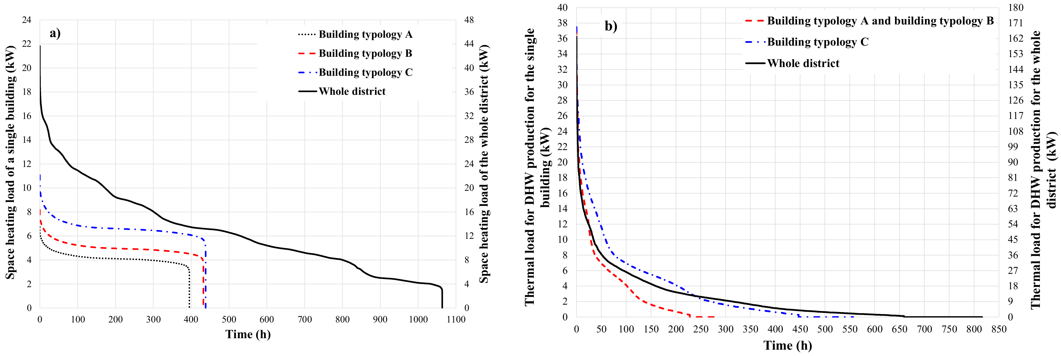
  • thermal load associated to the heating demand of the entire community (Figure 1a) has a duration of about 1063.5 h, with a maximum value of about 43.6 kW;
  • thermal load for DHW production of the district (Figure 1b) has a duration of about 816 h, reaching a largest value of 163.2 kW;
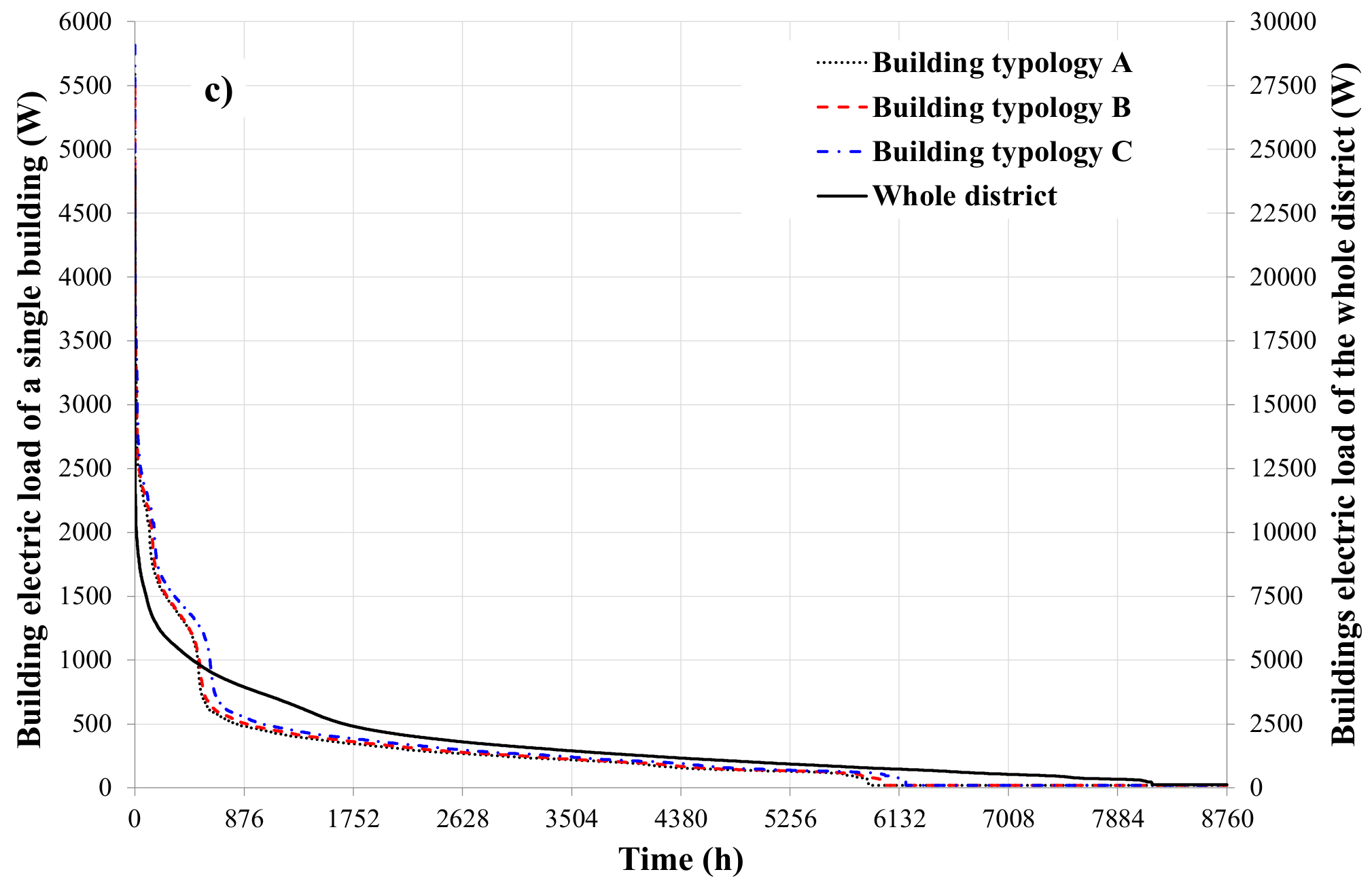
  • electric demand of all residential buildings (Figure 1c) has a duration of 8760 h, achieving a maximum of 24.2 kW.

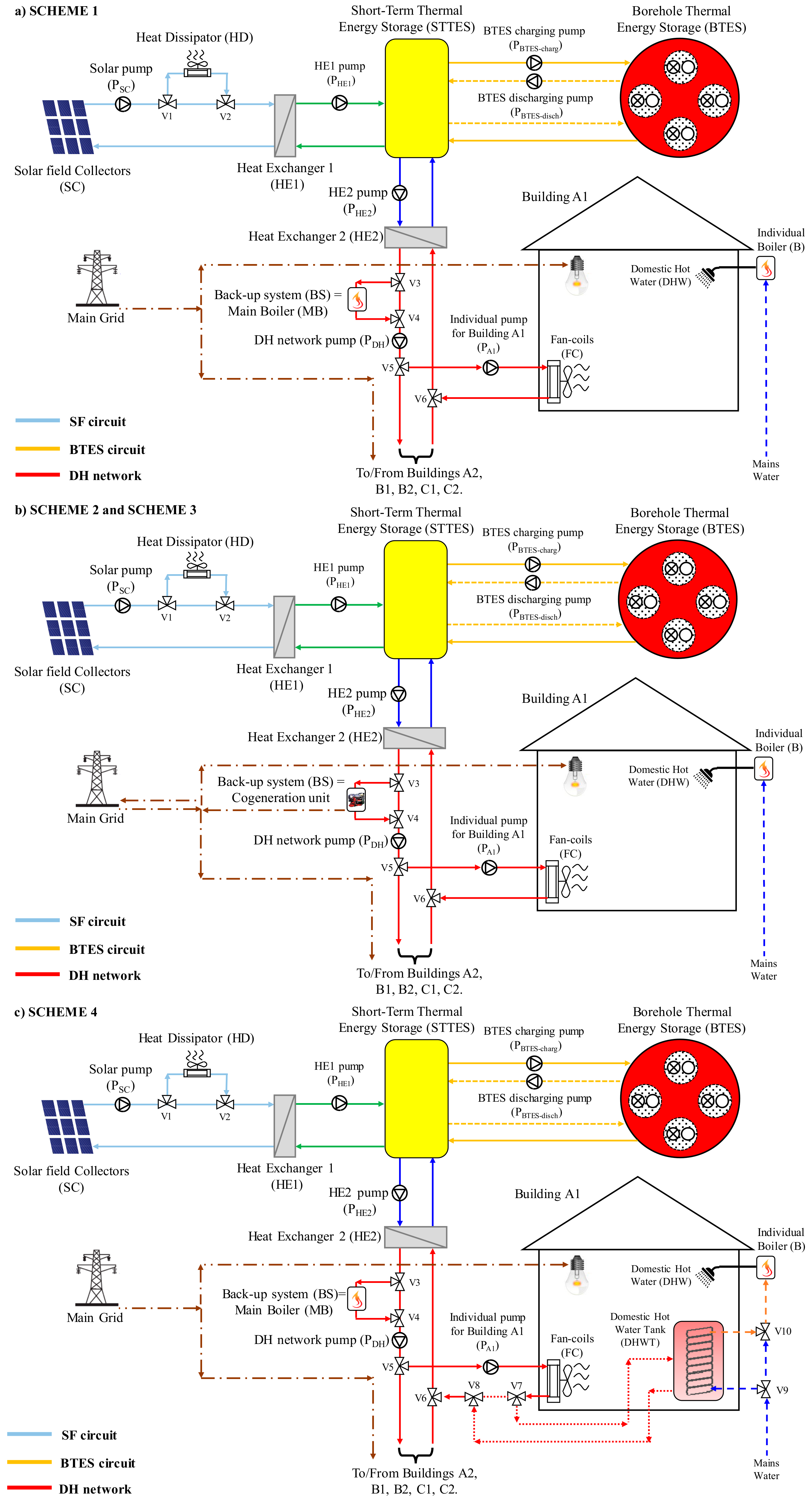
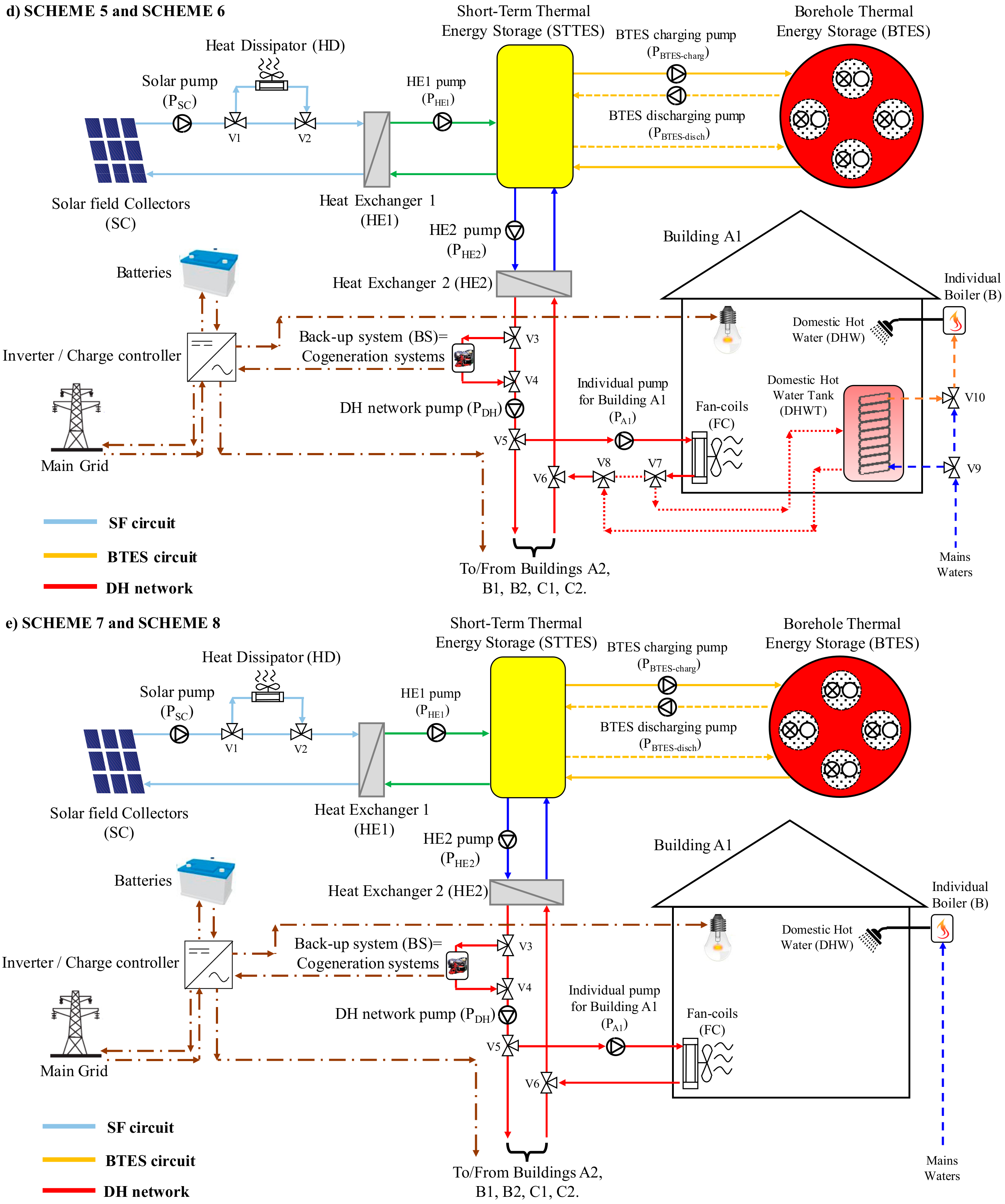
3. Description of the DH Network Configurations

The following 8 alternative schemes of a Central Solar district Heating Plant with Seasonal Storage (CSHPSS) are investigated: (1) SCHEME 1, (2) SCHEME 2, (3) SCHEME 3, (4) SCHEME 4, (5) SCHEME 5, (6) SCHEME 6, (7) SCHEME 7, and (8) SCHEME 8.
The schematics of the proposed configurations are reported in Figure 2a–e, where Figure 2a corresponds to the plant configuration named SCHEME 1, Figure 2b corresponds to both the plant configurations named SCHEMES 2 and 3, Figure 2c corresponds to the plant configuration named SCHEME 4, Figure 2d corresponds to both the plant configurations named SCHEMES 5 and 6, and Figure 2e corresponds to both the plant configurations named SCHEMES 7 and 8. In these figures, the following major components are indicated: end-users (6 houses), solar thermal collectors (SC), short-term vertical cylindrical thermal energy storage (STTES), seasonal single U-pipe borehole thermal energy storage (BTES), heat dissipator (HD), back-up system (BS), two counter-flow plate heat exchangers (HE1 and HE2), 6 local/decentralized individual non-condensing boilers (B) for DHW production (one per each building), 6 short-term DHW vertical cylindrical tanks (DHWT) integrated with an internal heat exchanger (IHE) to pre-heat the mains water (one per each building), fan-coils (FC), inverter/charge controller, electric batteries, pumps (P), 3-way valves and pipes.
The 8 proposed schemes exhibit some identical characteristics. In particular, whatever the CSHPSS configuration is:
  • the heat carrier fluid used in this paper is a mixture of ethylene glycol and water (40%/60% by volume) to achieve a boiling temperature of about 105 °C at 1 bar;
  • solar energy recovered by the solar collectors is firstly moved, thanks to the HE1, into the STTES;
  • excess solar energy is dissipated by blowing air through the HD (consisting of a finned coil heat exchanger) in the case of the temperature of the heat carrier fluid at the outlet of the solar collectors becomes larger than 95 °C;
  • in the case of space heating requirements, solar energy is moved from the STTES, by means of the HE2, into the fan-coils installed into the buildings via the distribution circuit to obtain the desired indoor temperature level during the heating period (15 November–31 March, according to [49]);
  • solar energy stored into the STTES can be moved into the BTES during the entire year (“BTES charging mode”) in the case of it is not instantaneously requested for space heating. Solar energy from the BTES can go back to the STTES (“BTES discharging mode”) only during the heating period with the aim of integrating the level of temperature inside the STTES. The direction of the heat carrier fluid is from the BTES center to the storage boundaries during the charging phase, with the aim of obtaining larger temperatures in the BTES center and smaller ones at the storage boundaries; the direction of the heat carrier fluid is inverted during the discharging phase;
  • when the solar energy stored into both the STTES and BTES is not able to fully cover the energy demands, a back-up auxiliary system is operated with the aim of supplementing the thermal energy needs in order to achieve the desired supply temperature level (55.0 °C);
  • the DHW is produced by means of 6 local individual boilers (B), one per house.
The proposed 8 configurations only differ in terms of:
(a)
back-up auxiliary system, and/or;
(b)
production of DHW, and/or;
(c)
utilization of electric energy storage.
The differences between the proposed schemes are specified and summarized in Table 3.
As reported in Figure 2a–e and Table 3, the following alternatives are considered with respect to the back-up system:
(a)
a 26.1 kWth Main condensing Boiler (MB) fueled by natural gas is utilized for both the SCHEMES 1 and 4;
(b)
2 parallel-connected 12.5 kWth natural gas-fueled MCHP units based on Internal Combustion Engine (ICE) are adopted for the SCHEMES 2, 5 and 7.
(c)
a 26.0 kWth natural gas-fueled MCHP device based on Stirling Engine (SE) is considered for the SCHEMES 3, 6 and 8.
The target of supply temperature for the distribution network is set to 55.0 °C; therefore, the auxiliary unit (MB or SE-MCHP or ICE-MCHP) is operated only when integrating the temperature level at the outlet of the heat exchanger HE2 is required to get the desired value. Therefore, the MCHP units are operated under a thermal-load following control logic according to the temperature level at the outlet of the HE2, providing their maximum thermal and electric outputs while activated. The electric energy provided by the MCHP systems is used to meet the electric demand; any excess of the MCHP electric output is charged into the batteries (if used) or sold to the power line; the electric storages (if used) and the central grid are also utilized to satisfy all peaks of electric demand.
As indicated in Figure 2a–e and Table 3, with reference to the DHW production, it can be noticed that:
(a)
the DHW is produced via 6 natural gas-fired non-condensing individual boilers only (one per house) for the SCHEMES 1–3, 7 and 8; in particular, the mains water enters the boilers and it is heated up to 45.0 °C;
(b)
for the remaining configurations (SCHEMES 4–6) the DHW is produced thanks to the operation of 6 natural gas-fired individual non-condensing boilers in combination with 6 local vertical cylindrical DHW tanks (one per building) equipped with one inlet, one outlet as well as one internal heat exchanger (IHE). In particular, during the heating period (15 November–31 March), mains water enters the heat exchanger immersed into the DHW tank, while the heat carrier fluid exiting the fan-coils is transferred into the DHWT with the aim of pre-heating the mains water. The individual boiler is activated with the aim of achieving the desired temperature of 45.0 °C only when the temperature of mains water exiting the heat exchanger is lower than the given target. During the remaining part of the year, the DHW at 45.0 °C is obtained through the 6 individual/decentralized boilers only, without using the DHWTs (as in the configurations SCHEMES 1–3).
As highlighted in Figure 2a–e and Table 3, three-series connected electric energy storages are used for the SCHEMES 5–8 (all including a micro-cogeneration system as back-up unit), while the batteries are not used for the remaining four configurations (SCHEMES 1–4). Whatever the season is (during both heating and cooling periods), the cogenerated electricity is firstly used to cover the electric load for the SCHEMES 5–8. In the case of the MCHP electric output is bigger than the electric demand and state of charge of the batteries is 100%, then the cogenerated electricity is sold to the central grid. In the case of the charge level of the electric storages is lower than the maximum (100%), then the eventual surplus of electric energy generation with respect the electric demand is charged into the batteries. In the case of the cogenerated electric output is not enough to fully satisfy the electric needs, the electric storages are discharged only when their state of charge is larger than 10%; the electric storages discharging is interrupted in the case their state of charge becomes smaller than 10%. The grid is used to cover all peaks of electric demand in the case of the cogenerated electricity is not enough to fully cover the electric demand and the state of charge of the batteries is lower than 10%.
In the case of the configurations with the main boiler as back-up system (SCHEMES 1 and 4), the electric demands are satisfied by means of the electricity provided by the electric grid only.
Table 4 describes and summarizes the principal characteristics of the leading components included in the proposed configurations reported in Figure 2a–e.

3.1. Simulation Models

Accurate numerical models are adopted to simulate the plant components in order to take into account (i) the occupant-driven loads and thermal behavior of buildings, (ii) the partial load operation of all components, (iii) the coupling between heating loads and simulation outputs of the components, and (iv) the logics controlling the operation of the plant.
The TRaNsient SYStems [44] environment is selected for modeling and analyzing the proposed plants during 5 years by setting a time step equal to 1 min. The length of the period of simulation (5 years) is selected with the aim of taking into account that it requires a significant time to totally charge the BTES; the first day of simulations is set to 1 January.
In the TRNSYS software, individual models (named “Types”) are used to model each sub-system. In this study, the Types are chosen from the TRNSYS library and calibrated based on information provided by the manufactures or data available in the literature. In the following the TRNSYS Types selected in the project for running the simulations of the proposed systems are briefly described.
The Type 56 is selected for modeling the thermal behavior of the buildings of the district.
The BTES is modeled by means of the Type 557a [57], i.e., the Duct ground heat STorage (DST) model, representing the state-of-the-art in modeling borehole heat exchangers (BHEs) [13]. In this model, the storage is characterized by a cylindrical shape with vertical symmetry axis. The layout of boreholes is fixed in a hexagonal shape and uniformly within the BTES field and the ground is assumed to be homogeneous. The top of the storage is covered with insulating material. The BTES numerical model is described in greater detail in [57]. Pärisch et al. [58] analyzed the performance of 3 double U-tube borehole heat exchangers with a depth of about 70 m by means of 2 h of experimental tests keeping constant the inlet temperature; the measured data have been compared to three different simulations models, including the DST model used in this paper. The results of the comparison between the measured outlet temperature and the outlet temperature predicted by the DST model highlighted how the predicted trend (i) follows the curve of measured inlet temperature, (ii) underestimates the thermal power injected in the borehole heat exchanger only during the first 0.25 h, (iii) is able to better approach the measured data in the remaining part of the simulation time. The authors selected the BTES volume (435.8 m3), the number (8), depth (12.43 m) and connection scheme (in series) of the boreholes thanks to the results of a large parametric analysis carried out in a previous paper [9]. In particular, concerning the configuration of the BTES, the authors investigated [9] the impacts of (i) the volume of the BTES, (ii) the depth of boreholes, (iii) the borehole heat exchangers (BHEs) number, as well as (iv) the BHEs type of connection on the performances of the solar DH plant while satisfying the energy demands of the same residential buildings; the values allowing to maximize the primary energy savings have been adopted. The thermal conductivities of soil and grout are defined based on information available in the current literature; in particular, Casasso and Sethi [59] indicated that thermal conductivity of soil could range between 0.5 and 3.0 W/mK, while thermal conductivity of grouting material can vary in the range 0.5 ÷ 5.0 W/mK.
The Type 534, selected for modeling the STTES, allows to divide the storage into 10 fully mixed equal sub-volumes with 10 isothermal temperature layers (top layer = node 1 and bottom layer = node 10) with the aim of taking into account the stratification in the storage. The tank model is detailed according to the data suggested by the manufacturer [51]. The authors selected the STTES volume (6.0 m3) thanks to the results of a large parametric analysis carried out in a previous paper [9].
The performances of DHWTs are also analyzed by using the Type 534; 10 isothermal temperature layers (where the bottom layer is 10 and the top layer is 1) are considered to take into account the stratification in the decentralized storages. Manufacturer specifications are taken into account to calibrate the numerical model [52].
The flat-plate solar collectors are modeled by means of the Type 1b. In more detail, the thermal efficiency of collectors is defined by the following equation:
η SC = 0.7484 16.17 T in , SC T amb / G
where G is the solar irradiation incident on collectors surface in kJ/hm2, Tamb is the ambient temperature, Tin,SC is the fluid inlet temperature. The values of 0.7484 and 16.17 hm2K/kJ are, respectively, the intercept efficiency and the efficiency slope. In the model, the intercept efficiency is adjusted for off-normal solar incidence by using the following incidence angle modifier K:
K = 1 b 0 S b 1 S 2
where S = (1/cosθ − 1) with θ being the incident angle for beam radiation, b0 = 0.103 and b1 = 0. The coefficients adopted in Equations (1) and (2) are defined according to manufacturer specifications [50]. The orientation and tilted angle of solar collector are selected for optimizing the performance with reference to the city of Naples. The values of the thermal efficiency of a single solar thermal collector measured by the manufacturer [50] according to the Standard [60] have been compared by the authors against the simulation values obtained by using the model (Type 1b) used in this work under the same operating conditions. The comparison indicated that the percentage differences between the manufacturer data and the outputs predicted by the model are very small (between a minimum of −1.52% up to a maximum of 1.14%) and, therefore, confirmed the suitability of the adopted model. The authors selected the area of the solar field (55.44 m2) thanks to the results of a large parametric analysis carried out in a previous paper [9].
The Type 511, representing a system for cooling a liquid by means of external air, is selected for modeling the heat dissipator.
HE1 and HE2 are simulated as counter-flow plate heat exchangers by using the Type 5b; an overall heat transfer coefficient, respectively, of 54.3 W/K per m2 of collector area for the HE1 and 25 W/K per GJ of heat demand for the HE2, are set based on the criteria indicated in [61].
As mentioned in the previous section, 3 alternative different auxiliary systems are analyzed in this work:
  • a 26.1 kWth condensing main boiler;
  • two parallel-connected 12.5 kWth ICE-MCHP units;
  • a 26.0 kWth SE-MCHP device.
First of all, the capacity required to the auxiliary back-up system in order to maintain the level of temperature at the outlet of the heat exchanger HE2 up to 55 °C (i.e., desired target of supply temperature) has been estimated by performing dedicated simulations by means of the software TRNSYS (with a time step of 1 min). The simulation results highlighted that the thermal power to be supplied by the back-up system to obtain 55 °C as supply temperature is always lower than 53.4 kW, and, in particular, is lower than 25.0 kW during 98% of simulation time. Therefore, the capacities of back-up units have been selected by considering devices commercially available on the Italian market and taking into account this simulation result.
The performance of the condensing main boiler (used in the configurations named SCHEMES 1 and 4)) is simulated in this paper by means of the Type 700 by considering its thermal efficiency (i.e., the ratio between thermal output and primary input of the unit) depending on the load factor (i.e., the ratio between the current and the maximum thermal outputs of the system). In particular, the following equation is implemented in the Type 700 for estimating the thermal efficiency of the condensing boiler:
η MB CSHPSS =   0.418 P th , out , MB CSHPSS / P th , nom , MB CSHPSS 2 + 0.7477 P th , out , MB CSHPSS / P th , nom , MB CSHPSS + 0.7284
where P th , out , MB CSHPSS is the thermal power supplied by the condensing boiler to meet the district needs and P th , nom , MB CSHPSS is the nominal thermal power of the condensing boiler (26.1 kWth). The experimental thermal efficiency of the selected condensing boilers is measured by Di Perna et al. [62] and compared by the authors against the predictions obtained by using Equation (3) upon varying the load factor. The comparison highlighted that the percentage differences between the measured performance and the simulation outputs are in the range −2.37% ÷ 4.8%, confirming the suitability of the model (Type 700) adopted in this study. According to the information reported by Di Perna et al. [62], a minimum turn-down ratio (defined as the ratio between the minimum and maximum capacities of the system) equal to 0.21 is assumed.
The decentralized non-condensing boilers used for producing DHW in all CSHPSS configurations have been simulated through the Type 700; a constant thermal efficiency of 90% is assumed according to the average performance of devices available in the current Italian market.
The operation of the MCHP devices (used in the SCHEMES 2, 3, 5 and 6) has been analyzed through the Type 907. Thomas [63] measured both the electric and overall efficiencies of the ICE-MCHP unit (model Dachs HKA G 5.5) and the SE-MCHP device (model SOLO 161) selected in this paper as a function of the supply temperature (with a constant return temperature). The electric efficiency ηel of a MCHP unit is defined as the ratio between the electric output and the primary input, while the overall efficiency ηtot is the ratio between the total (electric and thermal) output and the primary input; the difference between ηtot and ηel is the thermal efficiency, i.e., the ratio between the thermal output and the primary power input. The following regression equations are derived by the authors by interpolating the experimental overall efficiencies measured by Thomas [63] for both the SE-MCHP and ICE-MCHP units:
η tot SE - MCHP = 0.0007 T supply 2 0.0443 T supply 2 + 102.74
η tot ICE - MCHP =   0.00006 T supply 3 0.0134 T supply 2 + 0.8581 T supply + 77.106
where Tsupply is the temperature at the outlet of the MCHP devices.
The outputs of the above-mentioned equations have been compared with the experimental values measured by Thomas [63]. The comparison between the experimental data [63] and the predicted ones highlighted maximum deviations equal to about 1.90% and about −0.44% for the ICE-MCHP and the SE-MCHP devices, respectively. Therefore, Equations (4) and (5) have been implemented in the Type 907 and used in this project for predicting the performance of the MCHP devices upon varying the supply temperature.
The operation of the batteries is evaluated through the Type 47a, while the inverter/charge controller is simulated by means of the Type 48b [44]. The Type 47a allows to specify how the charge level of batteries changes as a function of the time, while the inverter converts the DC power to AC and supplies it to the load and/or feeds it back to cover the electric demand. The overall capacity of the 3 series-connected batteries (equal to 40.5 kWhel) is selected based on the procedure indicated by the manufacturer [56] as a function of the daily average overall electric requirement (equal to about 44.1 kWhel). Francis [64] investigated the performance of a solar-powered electric vehicle station including a Tesla Powerwall battery [56] with a capacity of 6.4 kWhel. Francis [64] measured the charge/discharge profiles of the 6.4 kWhel Tesla Powerwall along with the corresponding state of charge during the experimental validation in the Electric Sustainable Power Lab at TU Delft; the authors compared the curve representing the state of charge predicted by the Type 47a, used in this paper for modeling the batteries, against that one measured by Francis [64] in the case of same charging/discharging profiles; the comparison indicated that the percentage difference between predicted and measured states of charge is relatively small, ranging from 0% up to 6.7%, and, therefore, demonstrating the suitability of the adopted model.
The Type 742 is adopted for simulating the operation of the district heating network pump; the remaining pumps are analyzed through the Type 656.
The operation of the fan-coils is modeled by means of the Type 753d; this numerical model is detailed according to data provided by the manufacturer [65]. In particular, 5, 6, 8 fan-coils are considered inside the building types A, B and C, respectively. Each fan-coil is characterized by a nominal heating capacity of 0.65 kW as well as a nominal power consumption of 8 W (minimum fan velocity) based on manufacturer specifications [65].
The network of solar thermal collectors as well as the distribution circuit are modeled by considering a single pair of supply and return pipes. The pipes are modeled through the Type 31, where the heat losses are calculated by considering the heat loss coefficient equal to 0.05 kJ/hm2 K.
An EnergyPlus weather data file [66] is used for estimating the external climatic conditions associated to the city of Naples; the weather data are the same each year due to the fact that they are one year long.

3.2. Control Strategies

The heating period covers the period from 15 November up to 31 March, according to the Italian legislation related to the activation of heating systems in the city of Naples [49].
The mass flow rate of the heat carrier fluid ṁFC flows into the fan-coils only in the case of there is a call for thermal energy triggered by a thermostat installed inside the houses. The target of indoor air temperature Troom,set-point is set to 20.0 °C (with a deadband of 0.5 °C) only when at least one person being inside the houses during the heating period.
The recovery of solar power is performed depending on the temperature difference DTS = (TSC,out − T10,STTES) between the outlet temperature of the solar collectors TSC,out and the temperature T10,STTES at the node 10 of the STTES. In particular, the flow rate of the solar pump could vary with the time while the solar pump is on; the solar pump is activated and the mass flow rate achieves its lowest value (19.1 kg/h per m2 of gross area of solar collectors) when DTS is not lower than 10 °C; then, the flow of the solar circuit is modulated between the above-mentioned minimum and the maximum of 38.1 kg/h per m2 of gross area of solar collectors according to the value of DTS: when DTS is larger than 10.0 °C, the flow is automatically increased every time-step in order to guarantee DTS = 10.0 °C; the flow is automatically decreased every time-step if DTS is lower than 10.0 °C (but greater than 2.0 °C). The minimum and maximum values of the mass flow rate managed by the solar pump are defined according to the manufactured data of the solar collectors [50].
Whatever the plant configuration is, the flow into the HE1 pump is equal to that of one of the solar pumps.
The DH network pump is never deactivated, and it is always operated with a minimum flow rate in order to avoid a significant temperature drop/increase, even if there is no space heating demand. The flow rate of this pump is not constant, and it ranges between a minimum of 497.7 kg/h up to a maximum of 3782.7 kg/h. The maximum flow rate is set according to the nominal flow rates suggested by the fan-coils manufacturer [65] and it is achieved in the case of all fan-coils of all buildings are activated; the minimum flow rate is set according to the nominal flow rates suggested by the fan-coils manufacturer [65] by considering the case when all fan-coils of a single building (A1) only are activated.
Whatever the plant configuration is, the flow rate of the HE2 pump, when it is activated, is equal to that one corresponding to the DH network pump. In particular, the HE2 pump operates according to the temperature levels of hot and cold sides of the heat exchanger HE2 (Tin,HE2,hot, Tin,HE2,cold).
The target for the supply temperature of the distribution circuit is set to 55.0 °C; therefore, the back-up system (main condensing boiler of MCHP units) is activated/deactivated depending on the inlet and outlet temperature levels (Tin,MB/Tin,MCHP and Tout,MB/Tout,MCHP).
The set-point temperature to be achieved by the DHW mass flow rate ṁDHW is set to 45.0 °C; the decentralized boilers operate in order to produce DHW at 45.0 °C according to the inlet/outlet levels of temperature (Tin,B/Tout,B).
The BTES discharging/charging is operated depending on the temperature levels (T1,STTES and T10,STTES, respectively) at nodes 1 and 10 of the STTES, the temperature TBTES,center in the center of the BTES and the given set-point inside the houses Troom,set-point. A constant charging flow rate is set to the half of the minimum flow rate of the circuit of solar collectors (equal to 19.1 kg/h per square meter of gross area of solar collectors according to manufacturer data [50]); the discharging flow rate is not constant and it is assumed equal to that one flowing into the distribution network. The selection of the charging/discharging flow rates is based on the criteria suggested by Pahud [61]. Charging and discharging modes of BTES field are alternative; the BTES cannot be charged and discharged simultaneously.
Several studies demonstrated that operating the micro-cogeneration units under an electric-load following control strategy is not efficient and convenient. Therefore, the MCHP units are operated under a thermal-load following control logic; this means that the MCHP units are activated to achieve the given target temperature (55 °C) at the outlet of the heat exchanger HE2, providing their maximum thermal and electric outputs in the case of activation.
The electricity provided by the MCHP units is firstly transferred to the inverter/charge controller and then used to satisfy the electrical requirements, whatever the season is. The cogenerated electricity is sold to the central grid when the electric output of MCHP units becomes larger than the electric demand as well as the state of charge of the batteries is 100%. In the case of the charge level of the electric storages is lower than the maximum, then the possible excess of electric energy generation with respect the electric demand is injected into the batteries; when the electric production is not sufficient to completely satisfy the electric load, then the electric storages are discharged only when their state of charge is bigger than 10%; the discharging of the batteries is interrupted in the case their level of charge becomes lower than 10%. The grid is used to cover eventual peaks of electric demand in the case of the cogenerated electricity is not enough to fully cover the electric demand and the state of charge of the electric storage is lower than 10%.
Table 5 reports the main control logics adopted in this paper.

4. Description of the Heating System Assumed as Reference

A Conventional heating System (CS), representative of the current Italian scenario, is modeled and simulated (in TRNSYS environment) while satisfying the energy demands for space heating and DHW of the same district. In the heating system assumed as reference, each house is equipped only with a 26.6 kWth non-condensing boiler fueled with natural gas (modeled through the TRNSYS Type 700 by considering a constant thermal efficiency equal to 90.0%). The heat carrier fluid flows through radiators (modeled through the TRNSYS Type 1231) installed inside the houses. The system is operated with the same control logic used for the CSHPSS schemes. The target temperature of the boilers is set to 55.0 °C for space heating (with a deadband of 0.5 °C). The same profiles of DHW demand, occupancy and electric requirements adopted for the CSHPSS configurations are also used for the conventional system. The target for DHW production is set to 45.0 °C (similarly to the CSHPSS schemes). The electric requirements are fully covered through the electricity provided by the central grid.

5. Methods of Analysis

In this paper, the simulation results associated to the proposed plant are contrasted with the performance of the conventional heating system. The comparison is carried out by contrasting the consumption of primary energy, the equivalent emissions of carbon dioxide, the operation and capital costs.
In particular, the energy analysis is carried out by calculating the following parameter named Primary Energy Saving (PES):
PES   =   E p CS E p CSHPSS / E p CS
where E p CS is the primary energy consumption of the conventional system and   E p CSHPSS is the primary energy consumption of the CSHPSS schemes. The following formulas are used for calculating the PES:
E p CSHPSS = E th , MB / η MB + E p , MCHP + E th , DHW / η B + E el , import / η PP
E p CS   = E th , B / η B + E el , individual   pumps + E el , lighting + E el , domestic   appliances / η PP
where Eth,MB is the thermal energy supplied by the main condensing boiler, Ep,MCHP is the primary energy consumption of the MCHP devices, Eth,DHW is the thermal energy provided by the individual boilers for DHW production for the CSHPSS schemes, Eel,import is the electricity imported from the central grid for the CSHPSS schemes, Eth,B is the thermal energy provided by the individual boilers for both space heating and domestic hot water production in the case of the reference plant, Eel,individual pumps is the electric energy consumption of the individual pumps (PA1, PA2, PB1, PB2, PC1, PC2) of the reference plants, Eel,lighting is the electricity consumptionof the lighting systems of the reference plant, Eel,domestic appliances is the electricity consumption of the domestic appliances of the reference plant, ηMB is the thermal efficiency of the main condensing boiler [53], ηB is the thermal efficiency of the decentralized boilers [53], ηPP is the power plant average efficiency in Italy (the value of ηPP is considered equal to 0.42 according to the data suggested in [9,67] taking into account also the transmission losses). The values of Eel,import are calculated, time-step by time-step, as the difference between the overall electricity demand Eel,demand (due to the pumps, heat dissipator, fan-coils, the lighting systems as well as domestic appliances) and the electricity cogenerated by the MCHP units Eel,MCHP and/or provided by the batteries (Eel,batteries) in the case of Eel,demand > (Eel,MCHP + Eel,batteries).
The environmental impact associated to both the CSHPSS configurations and the conventional plant is assessed by means of the energy output-based emission factor approach indicated by Chicco and Mancarella [68]. In particular, the equivalent emissions of carbon dioxide are calculated and compared through the following parameter ΔCO2:
Δ CO 2 = m CO 2 CS m CO 2 CSHPSS / m CO 2 CS
where m CO 2 CSHPSS is the mass of equivalent emissions of carbon dioxide of the CSHPSS schemes and m CO 2 CSHPSS is the mass of equivalent emissions of carbon dioxide of the reference plant. The values of m CO 2 CSHPSS and m CO 2 CS are estimated as follows:
m CO 2 CSHPSS   = β E th , MB / η MB + E p , MCHP +   E th , DHW / η B + α E el , import
m CO 2 CS   =   β E th , B / η B + α E el , individual   pumps + E el , lighting + E el , domestic   appliances
where β is the CO2 equivalent emission factor related to the consumption of natural gas and α represents the CO2 equivalent emission factor associated to the electricity generation. In particular, α and β are set to 573 gCO2/kWhel and 207 gCO2/kWhp, respectively, according to the data indicated in [67,69] according to the current Italian scenario.
The comparison from an economic point of view is carried out firstly by contrasting the operation costs of the CSHPSS schemes with those associated to the conventional plant. The comparison is done by calculating the following parameter ΔOC:
Δ OC = OC CS OC CSHPSS / OC CS
where OC CS represents the operating costs of the reference plant and OC CSHPSS represents the operating costs of the CSHPSS schemes. The values of OC CS and OC CSHPSS are calculated as indicated below:
OC CSHPSS = UC ng E th , MB / LHV ng ρ ng η MB +   UC ng , MCHP E p , MCHP / LHV ng ρ ng + + UC ng E th , DHW / LHV ng ρ ng η B + UC el E el , import   -   UC el , sold E el , MCHP , exp
OC CS =   UC ng E th , B / LHV ng ρ ng η B + + UC el E el , individual   pumps + E el , lighting + E el , domestic   appliances
where UCng is the unit cost of natural gas consumed by the decentralized boilers [70], UCng,MCHP is the unit cost of natural gas consumed by the MCHP units [70], LHVng is the lower heating value of natural gas (equal to 49,599 kJ/kg representative of the scenario associated to the city of Naples) and ρng is the density of natural gas (considered equal to 0.72 kg/m3) [9], UCel is the unit cost of electricity purchased from the central grid [70], UCel,sold is the unit price of the electric energy sold to the central grid [71]. The tariffs are kept up-to-date according to the Italian market [70,71].
The values of UCng,MCHP are lower than the values of UCng [70] in Italy; this is a consequence of the fact that economic incentives are adopted by the Italian Government to support the diffusion of micro-cogeneration units [72].
In Italy, electricity tariffs that change as a function of energy time of use, in which the electricity costs are divided into more periods throughout the day based on the profile of the demand; this pricing structure provides price signals for the final users, aiming at shifting energy consumption to periods outside the utility expensive peak hours. In particular, the values of UCel depend on (i) the day of the week, (ii) the energy time of use during the day, (iii) the cumulated annual electric energy imported from the grid (in particular, four different intervals of consumption are specified: 0 ÷ 1800 kWhel, 1801 ÷ 2640 kWhel, 2641 ÷ 4440 kWhel, more than 4440 kWhel) and (iv) the region where the energy is consumed. Figure 3 indicates the weekly profile (from Monday to Sunday) of the unit cost of the electric energy purchased from the central grid (including the excise tax and the VAT) for the city of Naples according to [70].
According to the data reported in this figure, it can be underlined that the unit cost of the electric energy purchased from the central grid:
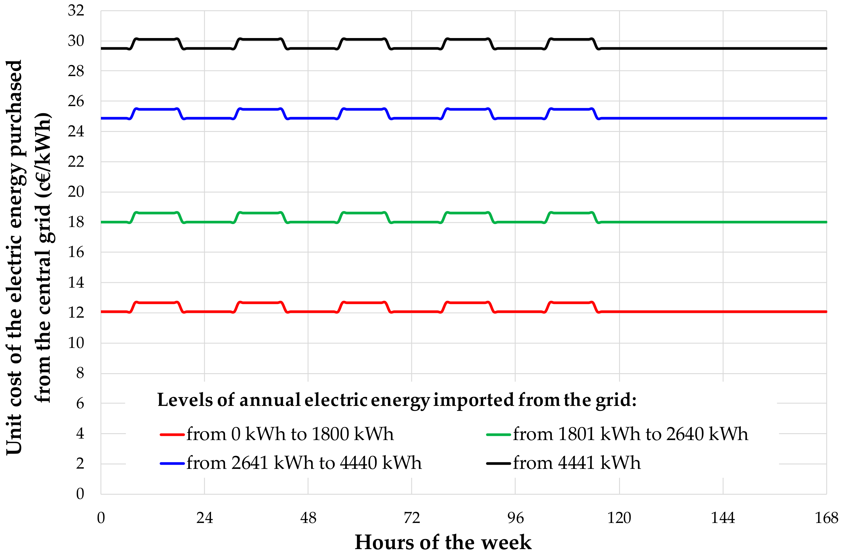
  • during the weekdays is larger or equal with respect to the values related to the weekends, whatever the cumulated level of annual electricity imported from the grid is;
  • increases at increasing the cumulated annual electric energy imported from the grid, whatever the hour and day are;
  • ranges between a minimum of 12.1 c€/ kWhel up to a maximum equal to 30.1 c€/ kWhel.
In this study, the unit price of the electric energy sold to the central grid UCel,sold is calculated month by month by means of the following formula according to the Italian scenario:
UC el , sold =   minimum PUN avg ;   PZ avg + UC Sf
where PUNavg is the monthly average national single price, PZavg is the monthly average zonal price and UCSf is the rate devoted to support electric energy generation from renewable sources and cogeneration devices. The values of PUN vary as a function of the hour, ranging between a minimum of 10 €/MWhel up to a maximum of 170 €/MWhel. The values of PZ depend on the hour of the day as well as the month of the year, varying between 32 €/MWhel and 78 €/MWhel. The value of UCSf is 47.51 €/MWhel in the case of the annual amount of electric energy sold to the grid is not larger than 1800 kWhel, while it is equal to 79.08 €/MWhel for an annual amount of electric energy sold to the grid bigger than 1800 kWhel.
The economic analysis is carried out also in terms of capital costs by calculating the so-called Simple Pay-Back (SPB) period, representing the time required to recover the extra initial investment cost. The following formula is used:
SPB   = CC CSHPSS CC CS / OC CS OC CSHPSS + EI CSHPSS
where CCCSHPSS is the capital cost of the CSHPSS schemes, CCCS is the capital cost of the reference system, EICSHPSS represents the economic incentives guaranteed by the Italian Government every year (for a maximum of 5 years), OCCSHPSS represents the operation costs of the CSHPSS (Equation (13)) and OCCS represents the operation costs of the conventional heating plant (Equation (14)). The maintenance costs are neglected.
The calculation of the difference (CCCSHPSS − CCCS), representing the extra investment cost of the proposed plant with respect to the conventional system, is carried out by means of the following formula:
CC CSHPSS CC CS = CC SC CSHPSS + CC SCpumps CSHPSS + CC STTES CSHPSS + CC BTES CSHPSS +   + CC BTESpump CSHPSS + CC MB CSHPSS + CC ICE - MCHP CSHPSS +   + CC SE - MCHP CSHPSS + CC DHnetwork CSHPSS + CC Batteries CSHPSS + CC DHWT CSHPSS
where CC SC CSHPSS is the investment cost of the solar field collectors (equal to 169 €/m2 in agreement with [73]), CC SCpumps CSHPSS is the investment cost of the solar field pumps (equal to 1488 € in agreement with the manufacturer data [74]), CC STTES CSHPSS is the investment cost of the short-term thermal energy storage (equal to 5651 € in agreement with the values suggested by Pahud [61]), CC BTES CSHPSS is the investment cost of the BTES equal to 22,917 € (calculated in agreement with the formula reported in [61] as a function of number and depth of boreholes, depth of the soil layer and thickness of the insulation on the top of storage, BTES area and borehole spacing), CC BTESpump CSHPSS is the investment cost of the BTES pump (equal to 2826 € in agreement with the manufacturer data [74]), CC MB CSHPSS is the investment cost of the main condensing boiler (equal to 1436 € in agreement with the data suggested in [75]), CC ICE - MCHP CSHPSS is the investment cost of the two internal combustion engine-based MCHP units (assumed equal to 44,000 € in agreement with the values suggested by Angrisani et al. [76]), CC SE - MCHP CSHPSS is the investment cost of the Stirling engine-based MCHP (equal to 38,950 € in agreement with the data reported in [77]), CC DHnetwork CSHPSS is the investment cost of both pipes and pumps included into the distribution network (equal to 14,500 € in agreement with the price list on public works of the Campania Region [78]) and CC DHWT CSHPSS is the investment cost of the 6 DHWT (equal to 2202 € based on the values suggested by Pahud [61]). The investment cost of the three electric batteries CC Batteries CSHPSS is equal to 18,984 € in agreement with the manufacturer data [56], i.e. about 468.7 €/kWhel; according to the scientific literature, this specific cost of selected batteries could make economically feasible the adoption of the electric storages.
With respect to the economic incentives, it should be underlined that the Italian Government has dedicated 55 billion € to address the economic consequences of Covid-19 lockdown. These measures include a jump supporting energy-efficient measures associated with such renovation projects, from 50% to 110% of capital costs up to a maximum of 30,000 € for each residential end-user [79]. Homeowners will have three ways in which to secure the eco-bonus: via the transfer of the tax-deductible allowance for installers and product suppliers, through the tax deduction for a period of maximum 5 years, and through invoiced discounts. In this paper, it is assumed EICSHPSS = 1.10·(CCCSHPSS − CCCS)/5 every year (up to a maximum of 30,000 € for each residential end-user [79]) by considering a tax deduction over a period of maximum 5 years. The decree is already in force and the economic incentive will be used to all expenses incurred between 1 July 2020 and 31 December 2021.

6. Results and Discussion

The CSHPSS schemes detailed in Figure 2a–d and Table 3 are modeled, simulated and evaluated with reference to a period of 5 years; the performances of the proposed configurations are contrasted with those of the reference plant (described in the Section 3) by using the parameters defined by Equations (6), (9), (12) and (15).
Table 6 reports the annual values of primary energy consumption (Equation (8)), equivalent emissions of carbon dioxide (Equation (11)) and operation costs (Equation (14)) for space heating, producing DHW as well as covering the electric demands of the conventional system. The weather data used in the simulation are one year long and, therefore, the simulation results are the same each year. The values reported in this table represent the baseline performance information of the conventional plant to be contrasted with those related to the proposed CSHPSS schemes.
Figure 4 indicates the values of PES (Equation (6)) upon varying the simulation year as a function of the plant configuration. This figure underlines that, whatever the plant configuration is, the PES greatly rises up from the first to the second simulation year; then, it becomes almost constant. Similar trends are derived for the parameters ΔCO2 (Equation (9)) and ΔOC (Equation (12)); therefore, the performance associated to the fifth simulation year can be considered as representative of a steady-state operation (whatever the scheme of the plant is).
The trends indicated in this figure are substantially related to the average temperature of the seasonal storage. Figure 5a indicates the average temperature of the ground in the storage volume Tavg,BTES as a function of the time during the first 2 years of operation, while Figure 5b reports the monthly amount of solar energy charged into the BTES and discharged from the BTES during the first two years of simulation. The results indicated in this figure correspond to the SCHEME 5 (that can be considered as representative of all plant configurations).
Figure 5 highlights that:
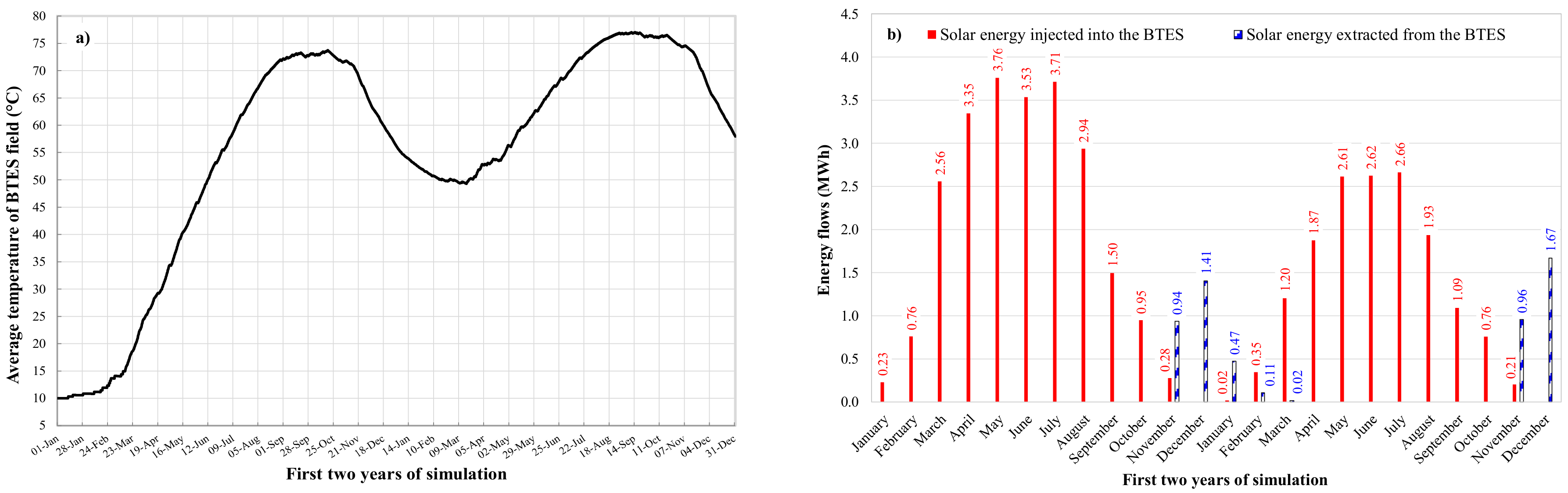
  • the average temperature of the BTES field is initially equal to 10 °C on 1 January and, after that, it rises up to about 73 °C during the summer of the first simulation year; then, it decreases (due to both heat losses and BTES discharging) during the heating season between the first and the second operation years, achieving a value of about 48 °C; finally, it increases again up to a maximum of about 77 °C during the summer of the second simulation year (Figure 5a);
  • heat discharged from the BTES field (only during the winter of the first two years of the simulation) reaches a maximum of about 1.67 MWh;
  • the solar energy injection into the seasonal storage occurs every month, except December; it increases up to reaching a maximum during May–July and then reduces; the largest value of solar energy charged into the boreholes is about 3.8 MWh during the first simulation year (in the second year it is lower due to the higher average temperature of the BTES field).
Figure 6 shows typical daily operation for the proposed 8 plant schemes during the same day (1 February of the fifth simulation year) in terms of thermal energy flows. In particular, Figure 6a–h corresponds to the SCHEMES 1–8, respectively. These figures indicate the values of net solar power recovered by the solar collectors, thermal power charged into the BTES, thermal power discharged from the BTES and thermal power supplied by the auxiliary system (boiler or MCHP units) as a function of the time. These figures highlight that: (i) the back-up system is often activated in order to compensate the lack of solar energy and maintain the desired supply temperature; (ii) BTES discharging generally occurs during the first part of the day to compensate the temperature levels in the STTES; (iii) BTES charging generally occurs during afternoons/evenings thanks to the solar energy previously stored into the STTES; (iv) solar energy recovered by the solar collectors increases with the time from about 9 a.m. up to reaching a maximum at about 12 a.m. and then reduces.
Figure 7 describes typical daily operation of the proposed plant configurations named SCHEMES 5–8 (the only four configurations including micro-cogeneration units as back-up system together with electric storages) during the same typical day (1 February of the fifth simulation year) in terms of electric energy flows; in particular, Figure 7a–d correspond to the SCHEMES 5–8, respectively. These figures shows the daily profiles of the electric power demand, the electric power generated by the micro-cogeneration devices, the electric power charged into the batteries, the electric power discharged from the batteries, the state of charge of the electric storages, the unit cost of electric energy purchased from the grid and the unit price of electric energy sold to the grid as a function of the time. These figures denote that:
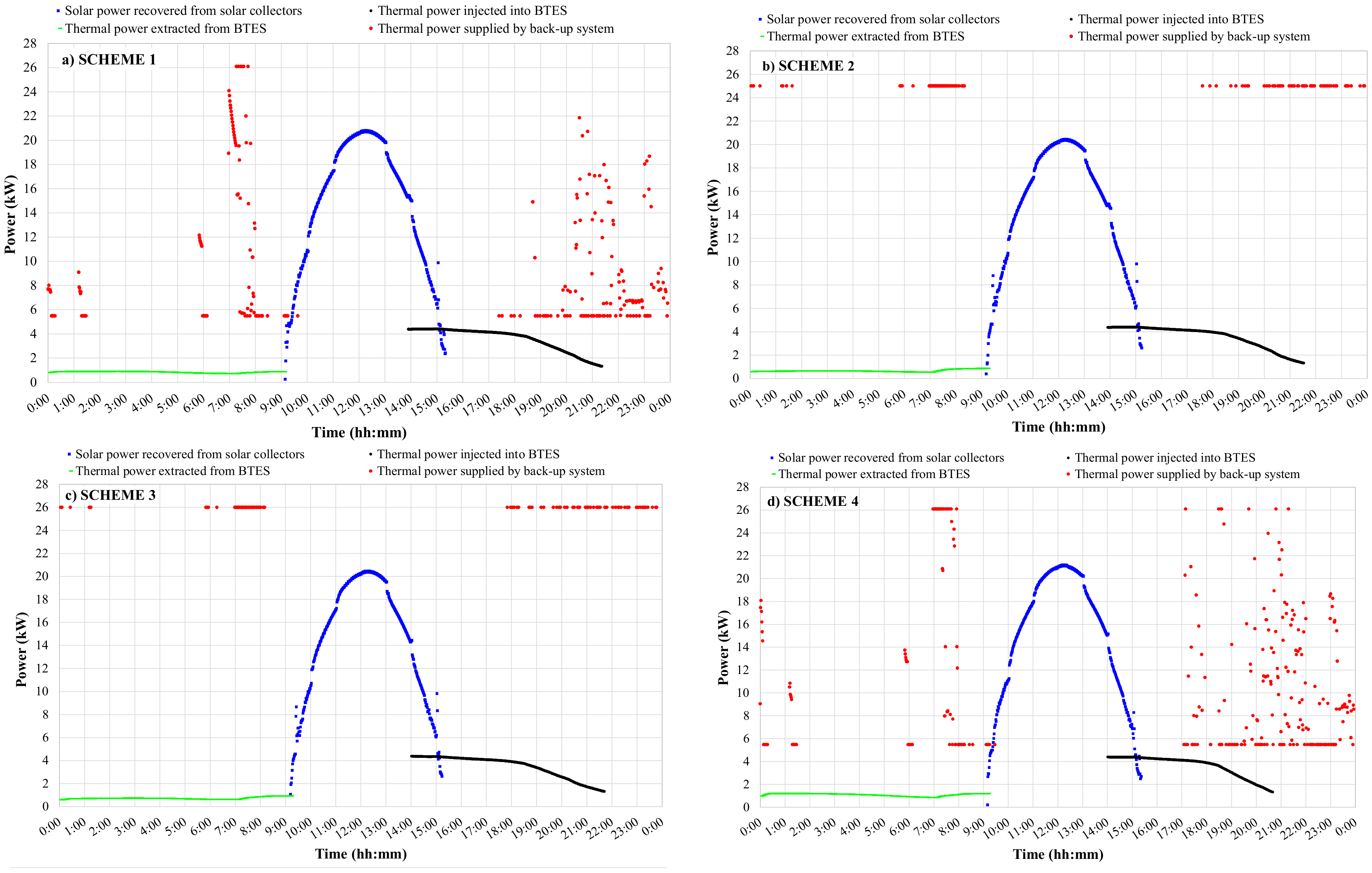
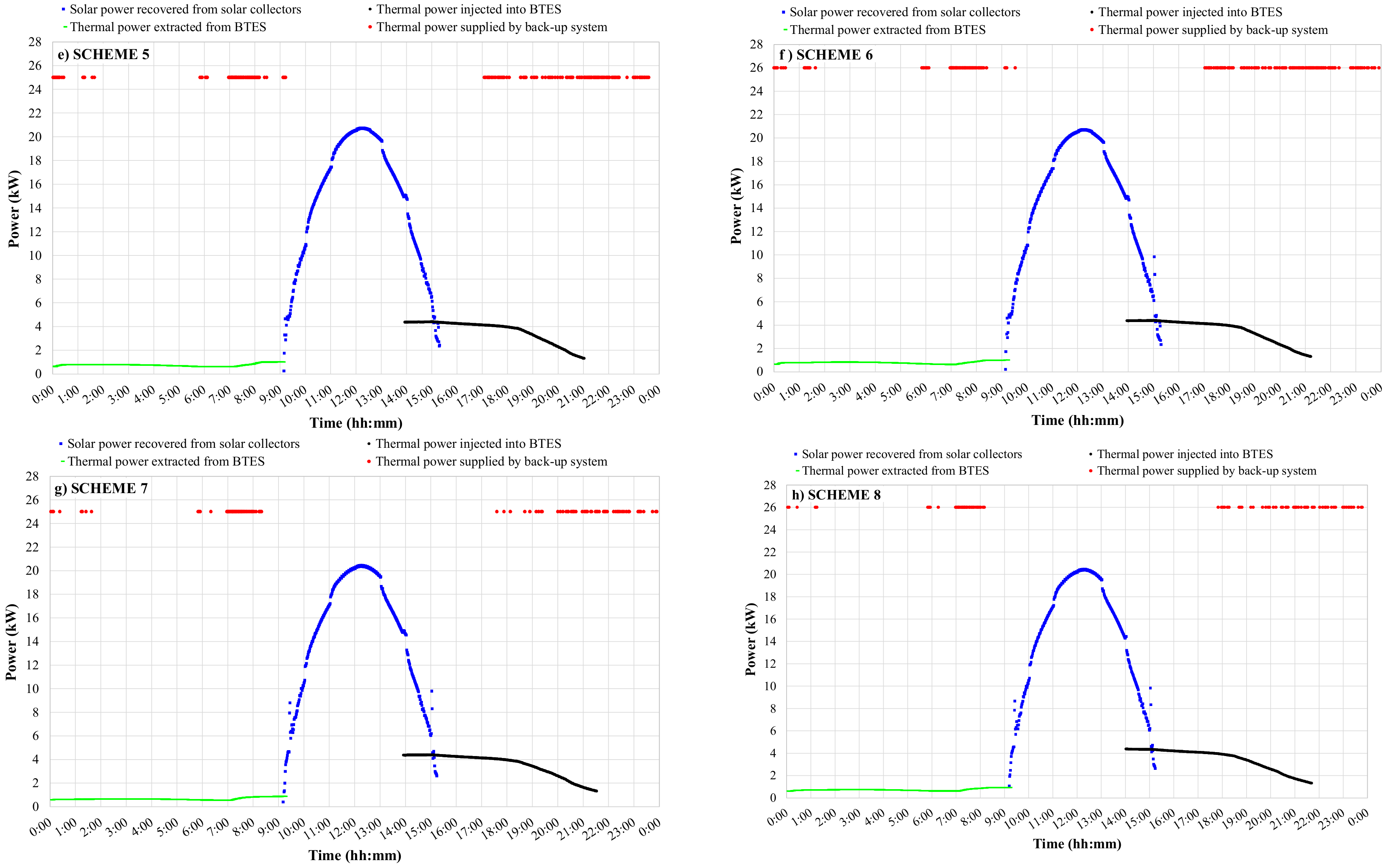
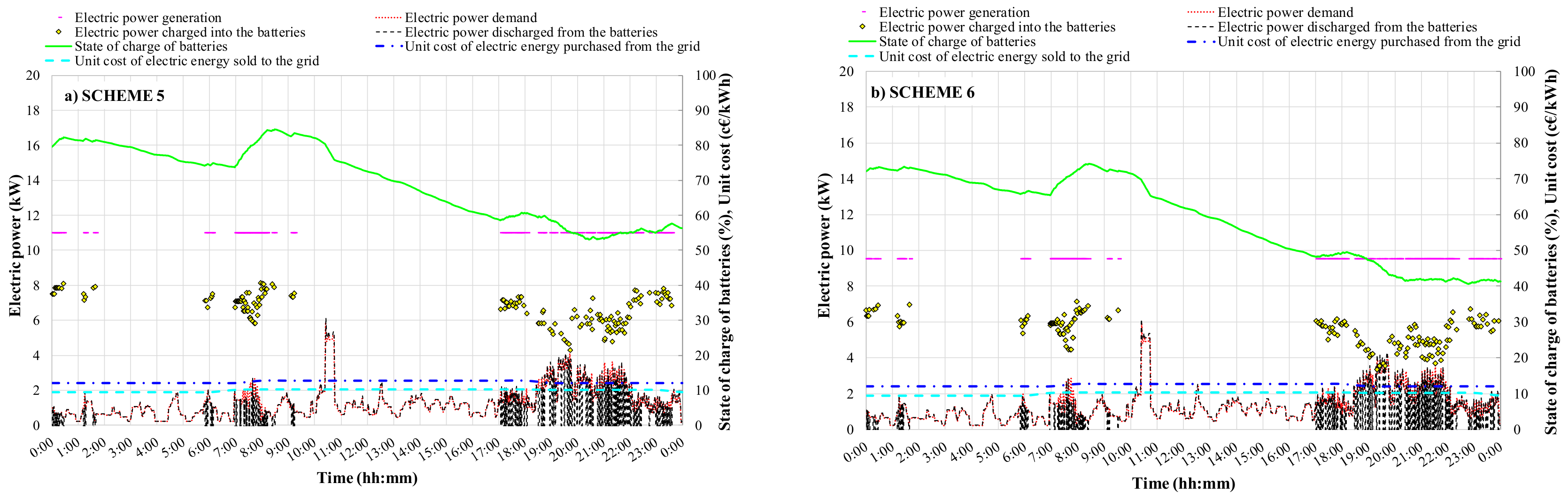
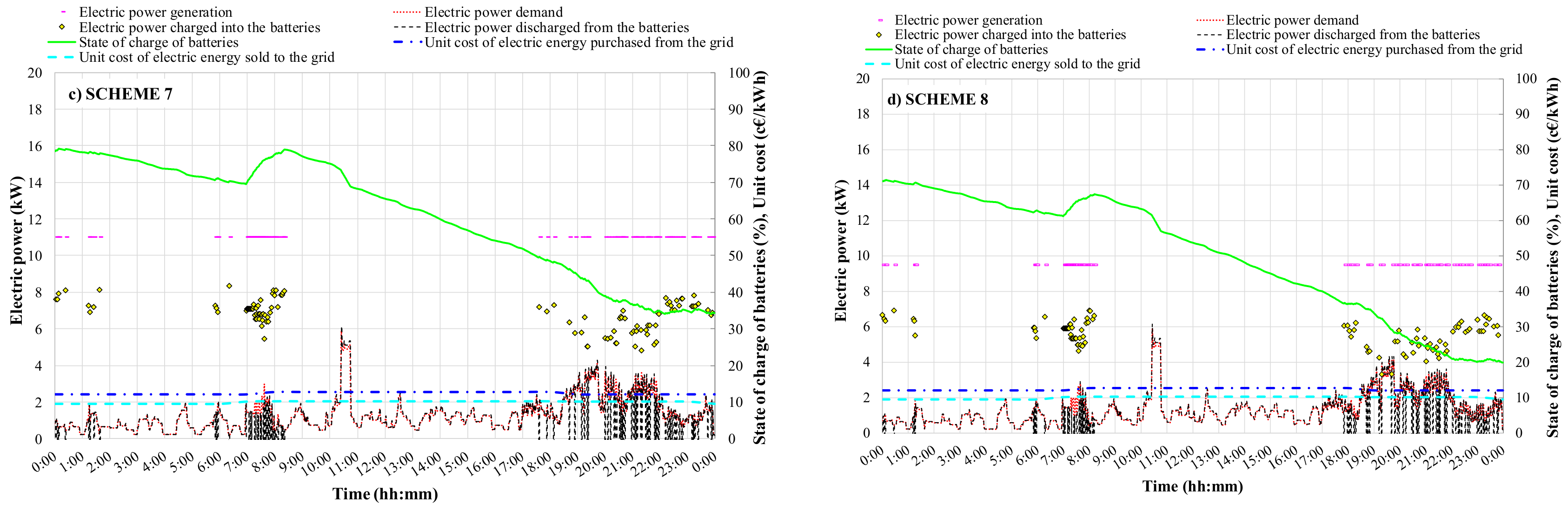
  • the electric power generation occurs according to the activation of the MCHP units (that are operated under a heat-led control logic in order to maintain the desired temperature level at the exit of the STTES) and corresponds to the nominal electric output of the cogeneration devices (11.0 kWel for the SCHEMES 5 and 7 and 9.5 kWel for the SCHEMES 6 and 8);
  • as detailed in the previous “Section 2. Description of the residential district”, the electric power demand is stochastic according to the models suggested by [45];
  • for the selected day, the electric power generation is always larger than the electric power demand when the MCHP devices are activated. Whatever the day is, the cogenerated electricity is firstly used to cover the electric load; in the case of the MCHP electric output is bigger than the electric demand and state of charge of the batteries is 100%, then the cogenerated electricity is sold to the central grid; the grid is used to cover eventual peaks of electric demand in the case of the cogenerated electricity is not enough to fully cover the electric demand and the state of charge of batteries is lower than 10%;
  • the charging/discharging of the batteries can occur during the entire year (both heating and cooling periods) depending on the levels of electric power cogenerated, electric power demanded as well as state of charge of the electric storages (as detailed in the previous “Section 3.2. Control strategies”). In particular, during the selected day the state of charge of the batteries is in the range 53.0% ÷ 84.5% for the SCHEME 5, in the range 40.0% ÷ 74.2% for the SCHEME 6, in the range 34.0% ÷ 79.2% for the SCHEME 7 and in the range 20.0% ÷ 71.5% for the SCHEME 8. The state of charge of the electric storages increases when the electric power production becomes larger than the electric power demanded and vice versa;
  • electric energy is not sold to the central grid during the selected day thanks to the fact that the state of charge of the electric storages is always lower than 100% and, therefore, there is always room to store the surplus of cogenerated electricity into the batteries;
  • during the selected day the electric energy demanded is not enough to fully discharge the batteries and, therefore, the state of charge of the electric storages is always larger than the given minimum (10%);
  • electric energy is not imported from the central grid during the selected day thanks to the fact that the state of charge of the electric storages is always larger than 10%. As a consequence, the required electricity can be discharged from the batteries in case of need;
  • the unit cost of electric energy purchased from the grid is larger than the unit price of electric energy sold to the grid, with a percentage difference ranging between 15.8% and 21.4% for the selected day during which the cumulated level of annual electricity imported from the grid is in the range 0 ÷ 1800 kWhel. With respect to this point, it should be considered that this percentage difference becomes more and more relevant at increasing the cumulated annual electric energy consumption (as detailed in the “Section 5. Methods of analysis” according to the Italian scenario [70]): (i) in the case of the annual electricity imported from the grid is in the range 1801 ÷ 2640 kWhel, then the above-mentioned percentage difference ranges between 43.4% and 47.2%; (ii) in the case of the annual electricity imported from the grid is in the range 2641 ÷ 4440 kWhel, then the above-mentioned percentage difference ranges between 59.0% and 61.8%; (iii) in the case of the annual electricity imported from the grid is larger than 4440 kWhel, then the above-mentioned percentage difference ranges between 65.5% and 67.8%. The annual electric energy consumptions of the single households served by the plant proposed in this study are larger than 1800 kWhel; as a consequence, the percentage of energy lost during the batteries charge/discharge process (due to the limited efficiency of the regulator (78%) and the inverter (96.0%)) is more relevant than the percentage difference between the unit costs of electric energy purchased/sold only during the first period of the year (up to the time where the annual electricity imported from the grid is in the range 0 ÷ 1800 kWhel); this is not true during the remaining part of the year, i.e., when the annual electricity imported from the grid becomes larger than 1800 kWhel.
Similar trends can be derived for the other days of the year, so that it can be stated that (i) it is worth to include an electric storage and (ii) the selected capacity of batteries (determined according to the manufacturer criteria [56]) is feasible.
Figure 8a reports the state of charge of the electric batteries (obtained every time-step as one of the outputs of the simulations) as a function of the time during the fifth simulation year for the SCHEME 5. Figure 8b shows the mean daily profile of the state of charge of the electric batteries, where each value is calculated as the arithmetic average (performed every time-step) of the state of charge of the batteries at the same time of different days by considering all days of the heating season only (when the MCHP units, and related electric generation, could be switched on) for the SCHEME 5. These figures demonstrate that:
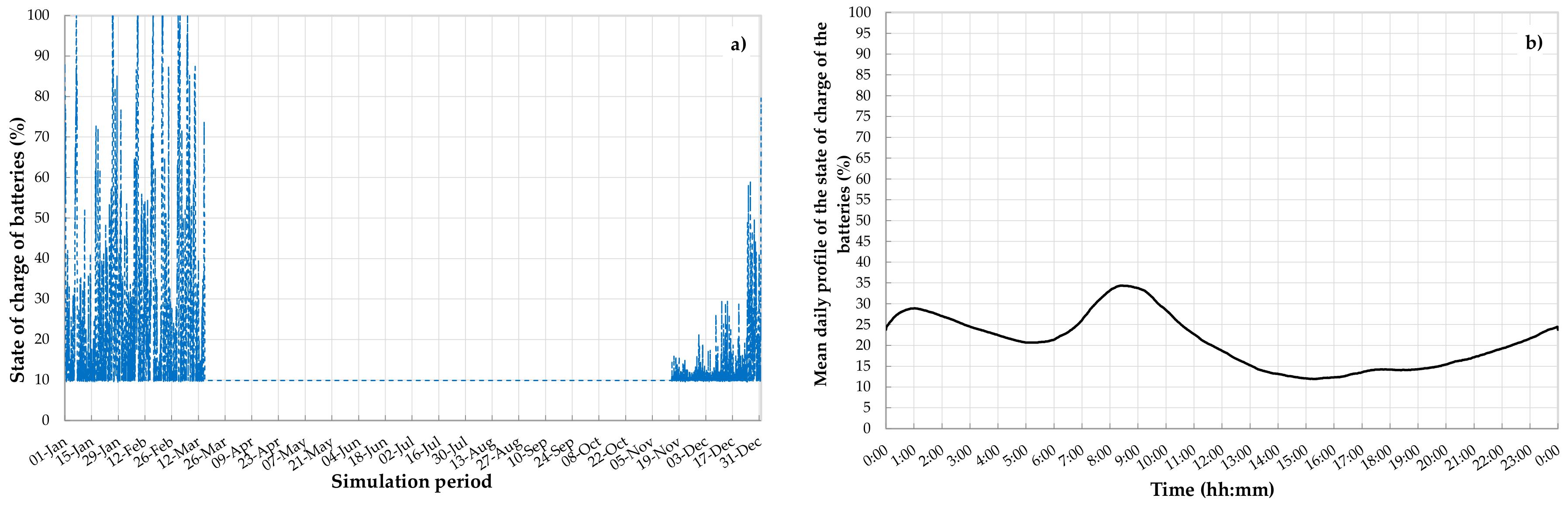
  • the state of charge of the batteries reaches the maximum value of 100% during several time-steps in the period between January and Mach (Figure 8a);
  • the mean state of charge of the batteries ranges between a minimum of about 11.9% and a maximum equal to about 34.3%; the maximum is obtained at 8:30 a.m., while the minimum is achieved at 3:20 p.m. (Figure 8b). The values of the mean state of charge of the batteries are affected by the limited daily operation time of the MCHP units during November and December because the BTES has been fully charged during the summer and, therefore, it has been able to provide the most part of thermal demand required to achieve the desired supply temperature;
  • the mean state of charge at first hours of the day (about 25%) is almost the same that at last hours of the day (Figure 8b).
Figure 9 indicates the values of PES, ΔCO2 and ΔOC during the fifth operation year (PES5th-year, ΔCO25th-year and ΔOC5th-year) upon varying the plant configuration. This figure underlines that:
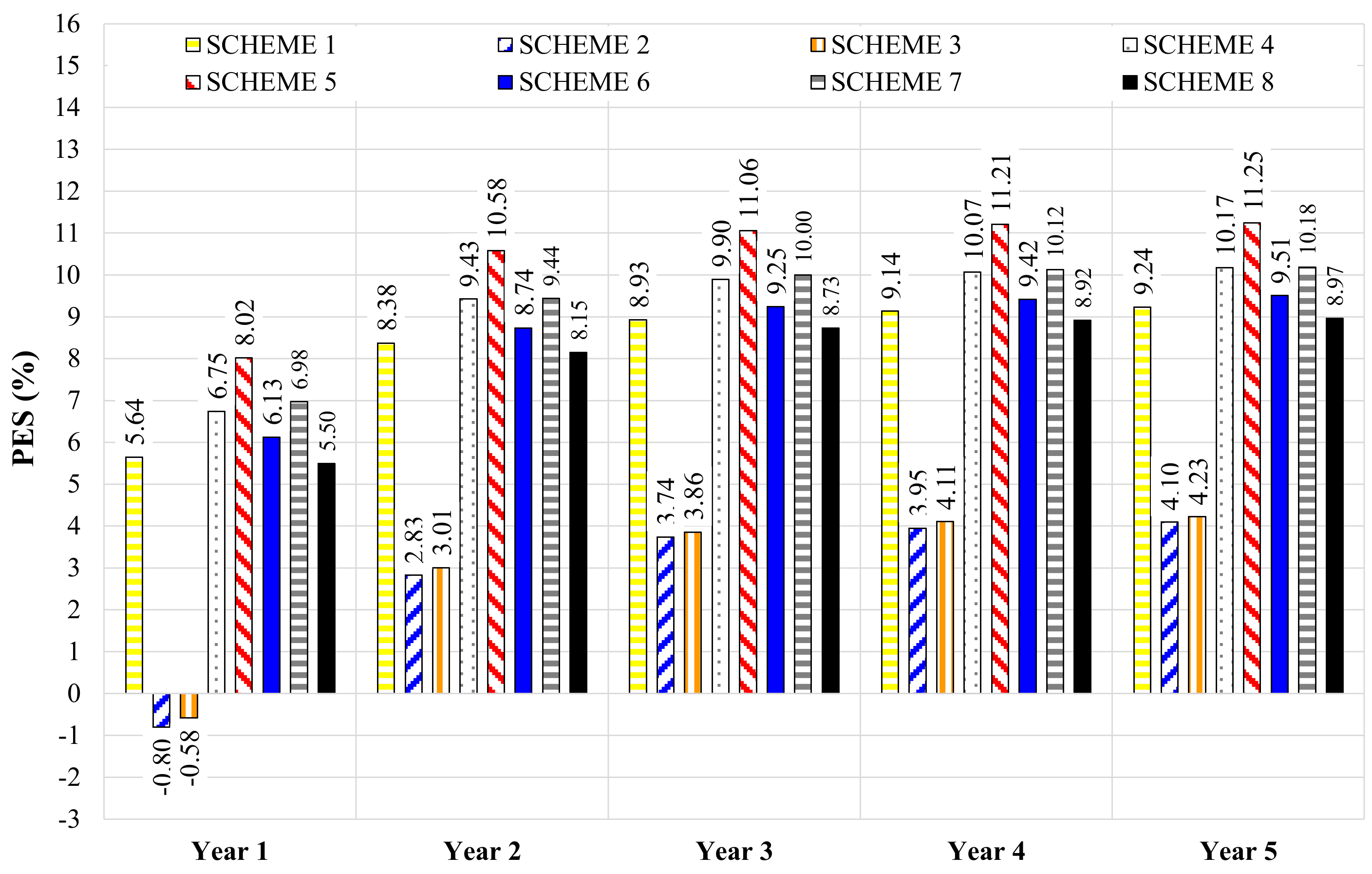
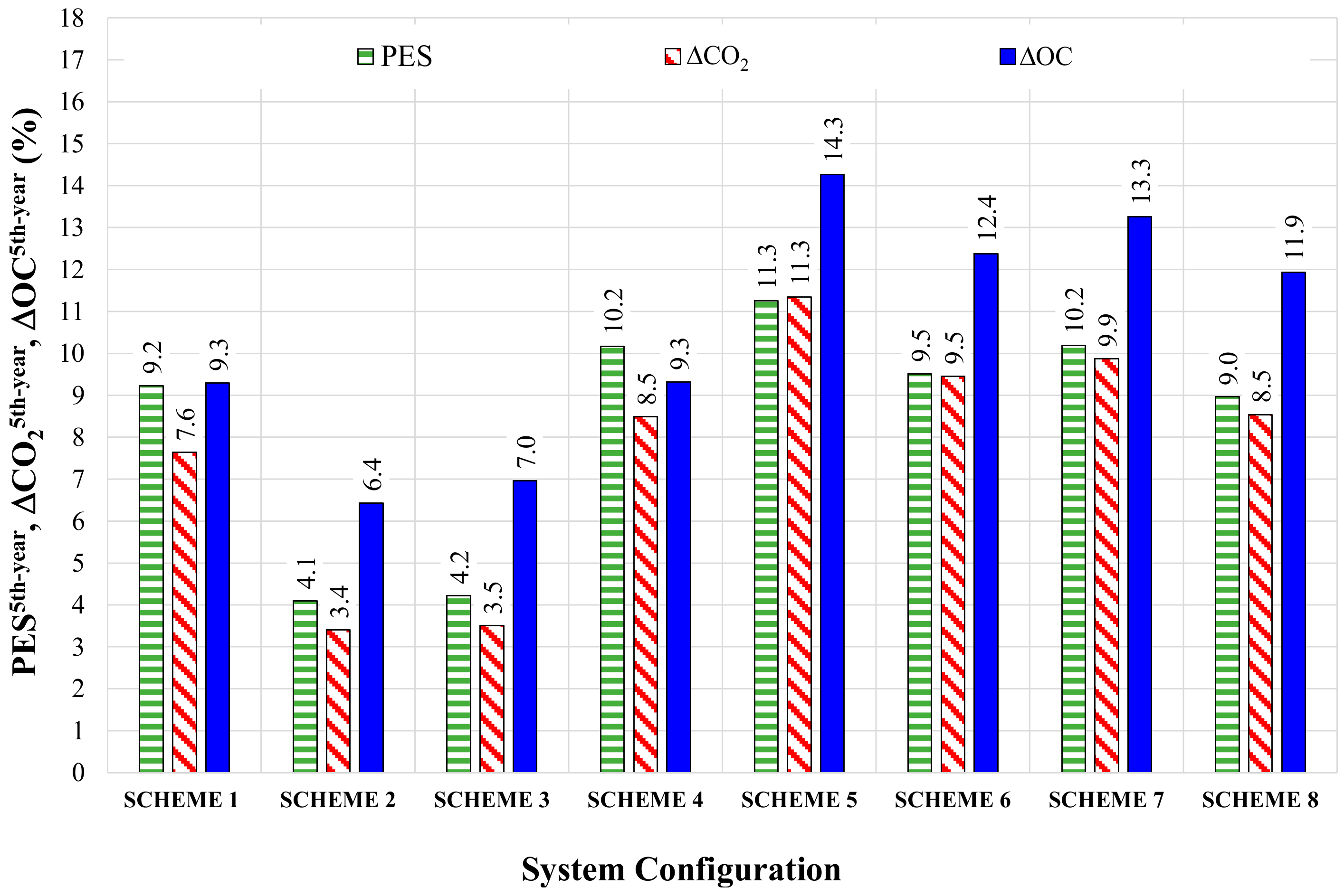
  • all proposed configurations are characterized by positive values of PES5th-year, ΔCO25th-year and ΔOC5th-year; this means that all schemes under investigation are able to decrease the consumption of primary energy, the equivalent emissions of carbon dioxide as well as the operation costs in comparison to the plant assumed as reference during the fifth operation year;
  • the largest and lowest values of PES are equal to 11.3% and 4.1%, respectively;
  • the minimum and maximum values of ΔCO2 are equal to 11.3% and 3.4%, respectively;
  • the largest and lowest values of ΔOC are equal to 14.3% and 6.4%, respectively;
  • the SCHEME 5 is that one allowing to obtain the best values of PES5th-year, ΔCO25th-year and ΔOC5th-year; in particular, with respect to the reference plant, this scheme allows to decrease the consumption of primary energy as well as the equivalent emissions of carbon dioxide by about 11.3%, while the operating costs are lowered by about 14.3% during the fifth year;
  • the SCHEME 2 is characterized by the lowest values of PES5th-year, ΔCO25th-year and ΔOC5th year; in particular, with respect to the conventional heating plant, in this case the consumption of primary energy, the equivalent emissions of carbon dioxide and the operation costs are reduced during the fifth year by about 4.1%, 3.4% and 6.4%, respectively;
  • the simulation data related to the SCHEMES 1–3 highlight that the best auxiliary unit is the natural gas-fired condensing boiler (when the DHW production is performed with the individual boilers only and the electric energy storage is not used); in particular, the values of PES5th-year, ΔCO25th-year and ΔOC5th-year are, respectively, about 2.3, 2.2 and 1.4 times larger in the case of the MB is adopted with respect to the cases when the MCHP units are considered; this is mainly due to the temporal mismatch between power generation of the MCHP units (operated under thermal load-following control logic) and electric requirement;
  • the comparison between the SCHEMES 2 and 3 shows that using the SE-based MCHP device allows to achieve slightly better performance with respect to the case when the ICE-based MCHP unit is adopted (in the case of DHW is produced with the individual boilers and the battery is not used) thanks to slightly higher overall efficiency of the SE-based system compared to that one of the ICE-based co-generator. However, the SCHEME 5 with the ICE-based MCHP unit is more advantageous than that one integrated with the SE-based MCHP device (SCHEME 6) in the case of both the electric energy storage is adopted and the DHW production is obtained by pre-heating the mains water through the DHWTs; this is because the electricity supplied by the ICE-based MCHP system and charged into the batteries (SCHEME 5) is about 1.3 times larger than that one related to the SE-based MCHP coupled with the electric storages (SCHEME 6);
  • the SCHEMES 7 and 8 are characterized by significantly larger values of PES5th-year, ΔCO25th-year and ΔOC5th year in comparison to SCHEMES 2 and 3, respectively. In particular, in comparison to the SCHEME 2, the SCHEME 7 allows to improve the values of PES5th-year, ΔCO25th-year and ΔOC5th year by about 2.5, 2.9 and 2.1 times, respectively; similarly, the SCHEME 8 enhances the values of PES5th-year, ΔCO25th-year and ΔOC5th year by about 2.1, 2.4 and 1.7 times, respectively, with respect to the SCHEME 3. These results demonstrate how adding the electric storages to the micro-cogeneration devices (without any other modification) greatly enhances the energy, environmental and economic performance of the plant mainly thanks to the self-consumption of MCHP electric output and, therefore, the reduced import of electricity from the central grid;
  • the comparison between the SCHEME 1 and the SCHEME 4 (differing only in terms of configuration for DHW production) shows that the domestic hot water production by pre-heating the mains water through the DHWTs increases the values of PES5th-year, ΔCO25th-year and ΔOC5th-year by about 1.10, 1.11 and 1.01 times, respectively; similar conclusions can be derived by contrasting the SCHEME 5 with the SCHEME 7 (the values of PES5th-year, ΔCO25th-year and ΔOC5th-year increase by about 1.1 times) as well as the SCHEME 6 with the SCHEME 8 (the values of PES5th-year, ΔCO25th-year and ΔOC5th-year improve by about 1.1, 1.1 and 1.0 times, respectively).
Figure 10 shows the main thermal energy flows of the CSHPSS schemes during the fifth operation year upon varying the configuration plant; in particular, the total solar energy falling on the tilted surface of thermal collectors (equal to 96.8 MWh, whatever the year is, due to the fact that the weather data are the same each year), the net solar energy recovered from the solar collectors, the thermal energy charged into the BTES field, the thermal energy discharged from the BTES field, the thermal energy supplied by the auxiliary unit (main boiler or MCHP units), the thermal energy supplied by the individual boilers for producing DHW are indicated.
Figure 11 highlights the main electric flows, i.e., the electricity cogenerated by the MCHP devices, the electric energy sold to the power line, the electricity charged/discharged into/from the electric storages, the electricity supplied by the MCHP units to directly cover the load and the electricity imported from the central grid upon varying the scheme of the plant during the fifth simulation year. In the same figure, the overall electric energy demand (16.2 MWh) associated to the operation of solar pump, heat dissipator, HE1 pump, HE2 pump, BTES charging/discharging pump, DH network pump, lighting and domestic appliances, individual pumps and fan-coils is also reported.
Figure 10 and Figure 11 show that:
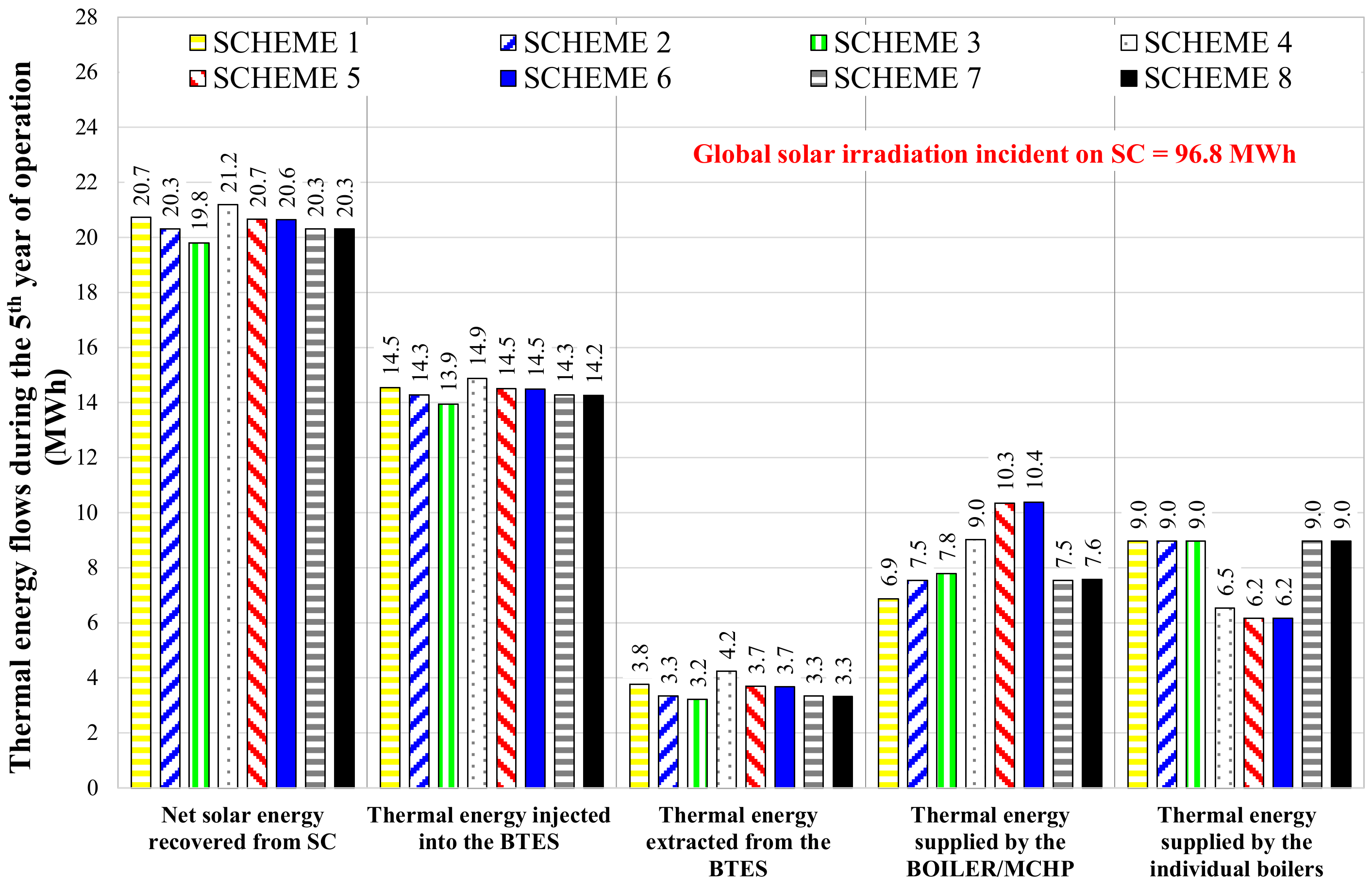
  • the configuration allowing to recover the largest amount of solar energy is the SCHEME 4, while the least significant solar energy recovery is that one associated to the SCHEME 3;
  • the annual average thermal efficiency of solar collectors, i.e., the ratio between the net solar energy recovered and the solar energy incident on the surface of collectors, ranges between a minimum of 20.5% (corresponding to the SCHEME 3) up to a maximum of 21.9% (corresponding to the SCHEME 4);
  • the efficiency of the BTES (defined as the ratio between the energy discharged from the BTES and the energy charged into the BTES) ranges between 23.1% and 28.6%, assuming the largest value for the SCHEME 4 and the lowest value in the case of the SCHEME 3. The values of BTES efficiency obtained in this paper are quite consistent with those found in the study carried out by Zhu and Chen [80]; in particular, they performed a huge sensitivity analysis on BTES performance under the climatic conditions of Tianjin (East Coast of China), characterized by a similar latitude with respect to Naples, upon varying the thermal conductivity of soil, the boreholes spacing and depth; they found a BTES efficiency (i) between 20% and 30% in about 17% of simulation cases, and (ii) lower than 50% in about 54% of investigated configurations;
  • the thermal energy supplied by the auxiliary device is the minimum one when the SCHEME 1 is considered, while it assumes the largest value for the SCHEME 6;
  • the thermal energy provided by the decentralized boilers for producing DHW is about 0.7 times lower for the SCHEMES 4–6 with respect to the SCHEMES 1–3, respectively; this is thanks to the fact that for the SCHEMES 4–6 the energy demand for DHW production is partially covered by pre-heating the mains water through the decentralized DHWTs;
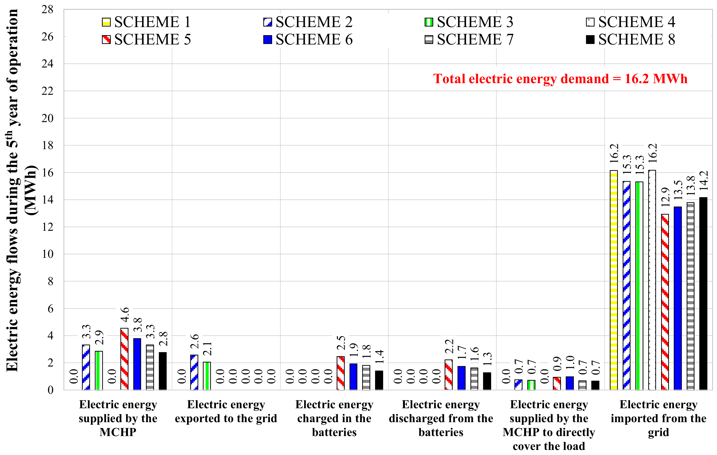
  • for the SCHEMES 2 and 3 the electricity imported from the central grid is about 0.95 times lower than that one associated to the case SCHEME 1 thanks to the cogenerated electricity partially covering the overall electric demand;
  • in comparison to the SCHEMES 2 and 3 (without the electric energy storages), respectively, the SCHEMES 7 and 8 (integrated with the batteries) allow to significantly decrease the import of electric energy from the central grid by about 10.2% and 7.6%, respectively.
  • the SCHEMES 5–8 (including micro-cogeneration units as back-up system together with electric storages) allow to avoid exporting the cogenerated electricity into the central grid with low revenues (so that the produced electric energy is directly used to cover the load or charged into the batteries).
With respect to the last point, it should be considered that, according to the Italian scenario, the values of UCng,MCHP range from a minimum of 0.43754425 €/Nm3 up to a maximum of 0.73602551 €/Nm3 depending on the cumulated level of natural gas annual consumption. Therefore, assuming both a lower heating value of natural gas equal to 49,599 kJ/kg (representative of the scenario associated to the city of Naples) as well as a density of natural gas equal to 0.72 kg/m3, the maximum value of UCng,MCHP in the case of the proposed application is around 0.022 € for producing 1 kWhel of electric energy by means of the micro-cogeneration devices investigated in this paper (according to the nominal electric and thermal efficiencies suggested by the manufacturers [53,54]). This means that the unit cost of electric energy cogenerated is lower than the unit cost of electric energy sold to the grid (about 0.097 €/kWhel) and, therefore, the losses of batteries charge/discharge process could be compensated, and the proposed application could be economically viable.
In addition, according to the Italian scenario [67,69], the proposed application also appears environmentally feasible taking into account that:
  • the equivalent emissions of carbon dioxide associated to the import of 1 kWhel of electric energy from the central grid are equal to 573 gCO2;
  • the equivalent emissions of carbon dioxide associated to the cogeneration of 1 kWhel of electric energy through the MCHP devices selected in this study are equal to about 62 gCO2.
The feasibility of batteries depends on several factors, such as electric demand profile as well as electric generation profile. Figure 12 reports the difference between the electric power produced by the microgeneration units and the demanded electric power as a function of the time with reference to the entire fifth year of operation of the SCHEME 5 (characterized by the best performances). The positive values of this difference represent the excess of power generation, i.e., the electric power that could be potentially charged into the batteries and/or sold to the central grid; the negative values in the graph are related to the electric power to be discharged from the electric storages and/or purchased form the central grid in order to cover the electric demand.
From this figure it can be recognized that:
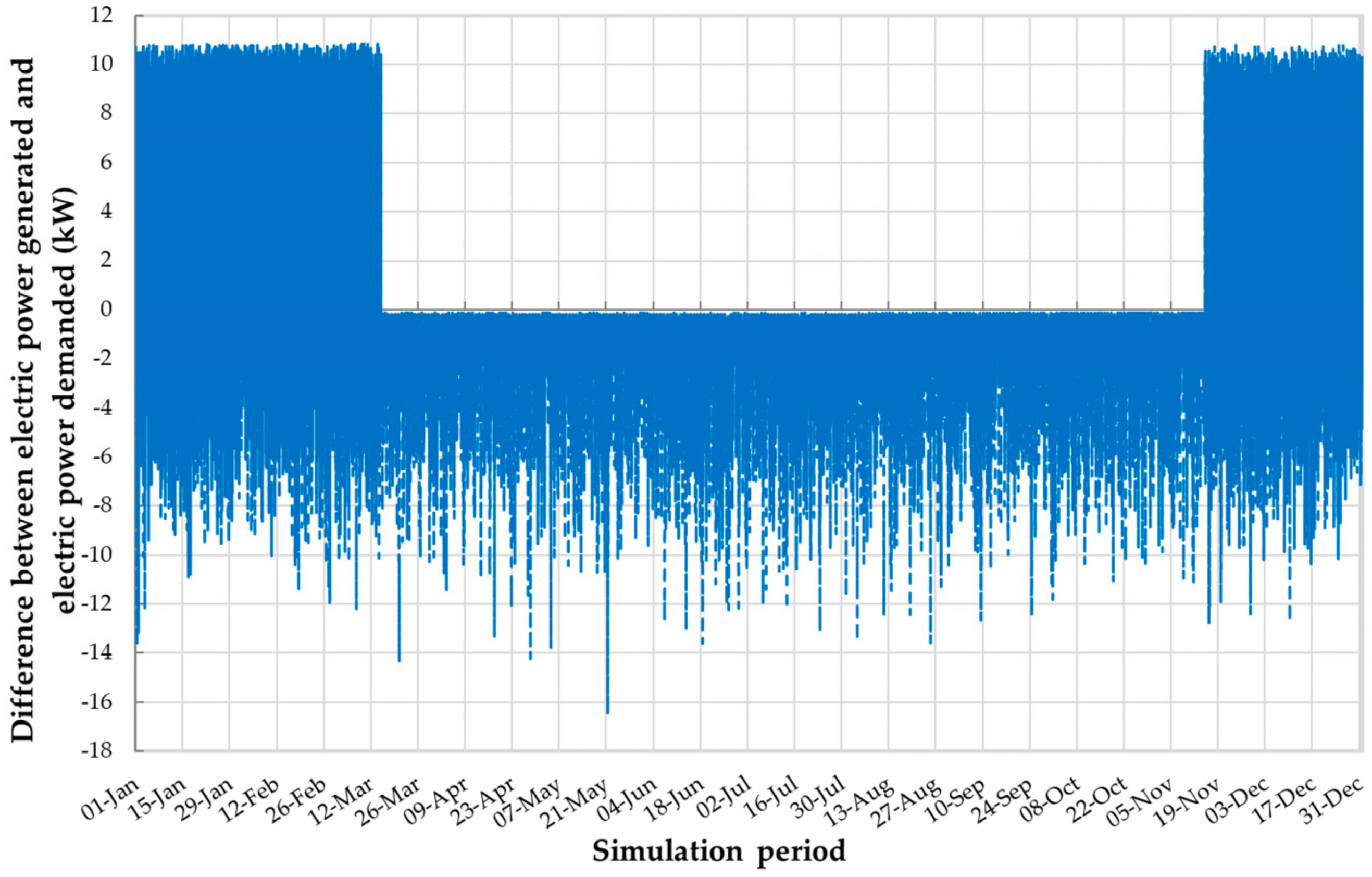
  • the maximum value is about 10.8 kW, while the minimum value is equal to about −16.5 kW;
  • there is an excess of electric energy generation (cogenerated electricity larger than demanded electricity) only during the heating period because of the fact that, as indicated in Table 5, the micro-cogeneration units (with associated electric output) can be activated only during this interval of time (under heat-led control logic); as a consequence, electric energy can be charged into the batteries and/or sold to the central grid only during the heating season;
  • during the cooling season the MCHP units are switched off and, therefore, the electric demand is almost entirely covered by the central grid.
The application of electric storages is also affected by cost unit cost of the electric energy purchased from the central grid UCel as well as the unit price of the electric energy sold to the central grid UCel,sold. In this study, the values of UCel vary between a minimum of 0.121 €/kWhel up to a maximum equal to 0.301 €/kWhel (according to the contents of Figure 3), while the average value of UCel,sold is about 0.097 €/kWhel. This means that the values of UCel are significantly larger that the values of UCel,sold, justifying the inclusion of electric storages into the plant schemes. In addition, it could be underlined that the Tesla Powerwall battery solution (adopted in this work) can be considered as a viable investment in regions where the values of UCel are over 0.25 €/kWhel according to [35].
The solar fraction SF5th-year of the CSHPSS is calculated as the ratio between the thermal energy demand that is covered thanks to the solar source and the overall thermal input to the CSHPSS schemes during the fifth operation year:
SF 5 th - year = E th , HE 2 CSHPSS / E th , HE 2 CSHPSS + E th , back - up CSHPSS + E th , DHW CSHPSS
where E th , HE 2 CSHPSS is the solar energy moved into the DH circuit by means of the heat exchanger HE2, E th , back - up CSHPSS is the thermal energy supplied by the auxiliary unit (main boiler or MCHP devices) and E th , DHW CSHPSS is the thermal energy provided by the decentralized boilers for producing DHW during the fifth simulation year. Figure 13 indicates the values of SF5th-year as a function of the configuration plant.
This figure shows that:
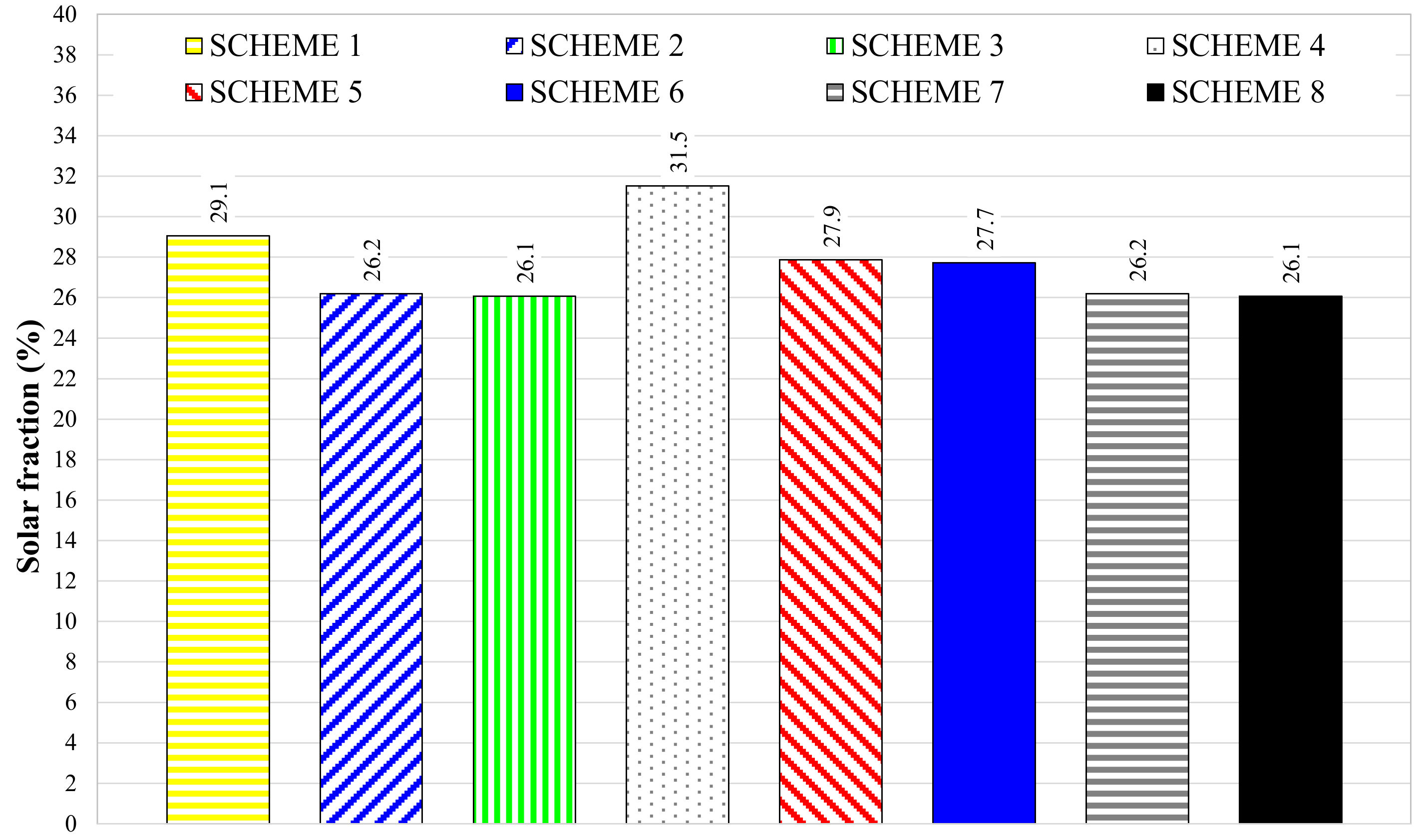
  • the largest value of SF5th-year, equal to 31.5%, is associated to the SCHEME 4 (using the boiler as auxiliary unit); this means that 31.5% of the overall thermal energy demand is satisfied by means of solar source in the above-mentioned configuration;
  • the lowest value of SF5th year is that one obtained for both the SCHEMES 3 and 8; it is equal to 26.1%.
The values of solar fraction found in this study are consistent with those associated to similar studies carried out under Italian climatic conditions [40,42,43], highlighting values of SF in the range between 28.2% and 80.0%.
Table 7 displays the values of the Simple-Pay Back (Equation (16)), i.e., the time required to recover the extra initial investment cost related to the CSHPSS schemes in comparison to the conventional scheme, as a function of the plant configurations.
This table underlines that:
  • the variation of SPB period is almost negligible upon varying the plant configurations, ranging from a minimum of 4.39 years (corresponding to the SCHEME 1) and a maximum of 4.49 years (corresponding to the SCHEME 2);
  • the proposed configurations are all feasible from an economic point of view thanks to the short time required to recover the investment.
With respect to the values reported in Table 7, it should be highlighted that they are greatly affected by the relevant economic incentives put in place by the Italian Government; without this support, the SPB periods would be much larger and the proposed configurations would not be economically feasible. In particular, the capital costs of the MCHP units are significantly consistent (about 44,000 € for the ICE-MCHP unit and about 38,950 € for the SE-MCHP device) and significantly contribute to the overall investment cost associated to the CSHPSS; the capital cost related to the BTES is also relevant, accounting for about 22,917 €.

7. Conclusions

During the last years, solar district heating systems achieved a great attention in the scientific community, with a significant number of worldwide applications, thanks to several benefits they can obtain with respect to decentralized plants. The review of scientific literature indicates that the studies carried out with reference to Italian applications are really limited and generally dated, with just two works [40,42] performed under climatic conditions associated to the southern Italy. Moreover, most of these studies are based on an energy analysis only, generally neglecting the economic as well as the environmental aspects. In addition, the size of the analyzed districts is significantly bigger than that one investigated in this work. Finally, the papers available in the literature are not focused on systems integrating cogeneration units and/or electric energy storages.
In this paper, the performances of a solar hybrid DH network including a seasonal borehole thermal energy storage are investigated during five years upon varying the auxiliary back-up system (boiler or micro-cogeneration units), with and without the utilization of electric energy storages in combination of the MCHP units; heat recovery from the distribution circuit for DHW production is also analyzed. The performances of the proposed plants have been contrasted with those of typical Italian decentralized heating plants.
The main scopes of the study can be summarized as follows:
  • the feasibility of micro-scale solar district heating networks in comparison to conventional heating systems in the case of Italian scenario;
  • the performance of long-term thermal storages in the case of micro-scale solar DH networks;
  • the most suitable back-up technology to be adopted into micro-scale solar district heating networks;
  • the capability of micro-cogeneration units in satisfying the requirement of electricity associated to small Italian district composed of residential buildings only;
  • the feasibility of batteries in improving the self-consumption of cogenerated electric energy and, consequently, decreasing the amount of power bought from the central electric grid;
  • the benefits deriving from the possibility to pre-heat the mains water for DHW production by recovering heat from the distribution circuit through decentralized tanks.
  • The comparison between the proposed plant configurations and the conventional heating system highlighted that:
  • all schemes are able to reduce the consumption of primary energy, the equivalent emissions of CO2 and the operation costs with respect to the reference system during the fifth operation year;
  • the largest reduction in terms of primary energy consumption, equivalent emissions of carbon dioxide and operation costs are equal to 11.3%, 11.3% and 14.3%, respectively;
  • the efficiency of the seasonal storage is significant, ranging between 23.1% and 28.6%;
  • the largest solar fraction achieved during the fifth simulation year is about 31.5%;
  • in the case of the batteries are not used, the best auxiliary technology is the natural gas-fired condensing boiler;
  • the configuration using the ICE-based MCHP device as back-up system coupled with the batteries and pre-heating the mains water through the heat recovery from the district network (SCHEME 5) is that one allowing to obtain the largest savings;
  • the thermal energy provided by the decentralized boilers for producing DHW is about 0.7 times lower for the 3 configurations where the pre-heating of mains water is performed through the heat recovery from the district network in comparison to the cases where the domestic hot water production is based on the operation of individual boilers only;
  • with respect to the schemes using the MCHP units without the batteries, the addition of the electric energy storages only allows to significantly reduce the import of electricity from the central grid, the equivalent emissions of carbon dioxide and operation costs up to 1.1, 2.9, and 2.1 times, respectively;
  • the proposed schemes are economically feasible (SPB periods of about 4.5 years) mainly thanks to the significant economic incentives put in place by the Italian Government.
In the future, the authors would extend this work to consider the integration with eco-friendly chillers that could be driven by solar energy (such as adsorption units) with the aim of covering the cooling demand of the district and assess its energy, environmental and economic feasibility with respect to conventional heating and cooling systems. In addition, one of the next research steps would consider the utilization of excess of electrical energy generation (produced energy less demanded energy) to power vapor-compression electric heat pumps instead of adopting electric storages. Moreover, future researches will be also focused on the potential application of the proposed schemes under different operating scenarios upon varying the buildings loads and/or the climate conditions. Finally, the assessment of environmental impact will be performed by means of a life-cycle analysis (LCA) in order to take into account all the stages of the life-cycle associated to the proposed components.

Author Contributions

Conceptualization, A.R., A.C. and S.S.; methodology, A.R., A.C. and S.S.; software, A.R., A.C., G.C. and M.S.; validation, A.R., A.C., G.C. and M.S.; formal analysis, A.R. and A.C.; investigation, A.R., A.C., G.C. and M.S.; resources, A.R. and S.S.; writing—original draft, A.R., A.C., G.C., M.S. and S.S.; writing—review and editing, A.R., A.C., G.C., M.S. and S.S.; visualization, A.R., A.C., G.C. and M.S.; supervision, A.R. and S.S.; project administration, A.R.; funding acquisition, A.R. All authors have read and agreed to the published version of the manuscript.

Funding

This work was undertaken as part of the research project titled “Solar smart Energy Networks integrated with borehole thermal Energy storages serving small-scale districts in the Campania region”—S.E.N.E.CA. (CUP: B68D19001880005) funded by the “V:ALERE 2019 program” of the University of Campania Luigi Vanvitelli (Italy). The article processing charge for publication in this open access journal was funded by the “V:ALERE 2019 program” of the University of Campania Luigi Vanvitelli (Italy).

Conflicts of Interest

The authors declare no conflict of interest.

Nomenclature

Latinletters
ACalternating current
Bindividual boiler
BATbatteries
BHEborehole heat exchanger
BTESborehole thermal energy storage
BSback-up auxiliary system
CCcapital cost (€)
CO2equivalent emissions of carbon dioxide
CSconventional system
CSHPSScentral solar heating plant with seasonal thermal storage
DCdirect current
DHdistrict heating
DHWdomestic hot water
DHWTdomestic hot water tank
DSTduct ground heat storage
Eenergy (MWh)
EIeconomic incentives (€/year)
EUEuropean Union
FCfan-coils
Gsolar irradiation (kJ/hm2)
HDheat dissipator
HE1heat exchanger 1
HE2heat exchanger 2
ICEinternal combustion engine
ICE-MCHPinternal combustion engine-based MCHP device
Kincidence angle modifier
LHVlower heating value (kJ/kg)
mmass (kg)
m ˙ . ss flow rate (kg/h)
MBmain back-up condensing boiler
MCHPmicro-combined heat and power
OCoperation cost (€)
Ppower (kW)/pump
PESprimary energy saving (%)
PUNnational single price (€/kWh)
PVphotovoltaic
PZ zonal price (€/kWh)
SCsolar field collectors
SEStirling engine
SE-MCHPStirling engine-based MCHP device
SFsolar fraction
STTESshort-term thermal energy storage
Ttemperature (°C)
Tmmean temperature between the inlet and outlet temperature of the SC (°C)
UCunit cost (€/kWh, €/m3)
UCSfrate devoted to support electric energy generation from renewable sources and cogeneration devices (€/kWh)
V3-way valve/Volume (m3)
Greeks
αCO2 equivalent emission factor for electricity production (kgCO2/kWhel)
βCO2 equivalent emission factor of coal-burning (kgCO2/kWhp)
difference
ηefficiency (-)
λthermal conductivity (W/mK)
θ:incident angle for beam radiation (°)
ρdensity (kg/m3)
Superscripts/Subscripts
1node 1 at the top of the STTES
10node 10 at the bottom of the STTES
5-yearreferred to the fifth year of simulation
ambambient
avgaverage value
Bindividual boiler
batteriesbatteries
BTESborehole thermal energy storage
centercenter of the borehole thermal energy storage
chargcharging
CO2carbon dioxide equivalent emissions
coldload side
CSconventional system
CSHPSScentral solar heating plant with a seasonal storage
DHdistrict heating
DHWdomestic hot water
dischdischarging
elelectric
expexported to the electric grid/experimental
FCfan-coils
HDheat dissipator
HE1heat exchanger 1
HE2heat exchanger 2
Hotsource side
IHEinternal heat exchanger
importelectric energy imported from the national electric grid
ininlet
MBmain back-up condensing boiler
ngnatural gas
nomnominal
outoutput/outlet
pprimary
PPpower plant
predpredicted
roomindoor environment
SCsolar field collectors
set-pointtarget temperature
soldelectric energy sold to the national electric grid
STTESshort-term thermal energy storage
ththermal
tottotal/overall

References

  1. Sayegh, M.A.; Danielewicz, J.; Nannou, T.; Miniewicz, M.; Jadwiszczak, P.; Piekarska, K.; Jouhara, H. Trends of European research and development in district heating technologies. Renew. Sustain. Energy Rev. 2017, 68, 1183–1192. [Google Scholar] [CrossRef] [Green Version]
  2. Hiltunen, P.; Syri, S. Highly renewable district heat for Espoo utilizing waste heat sources. Energies 2020, 13, 3551. [Google Scholar] [CrossRef]
  3. Büchele, R.; Kranzl, L.; Hartner, M.; Hasani, J. Opportunities and challenges of future district heating portfolios of an austrian utility. Energies 2020, 13, 2457. [Google Scholar] [CrossRef]
  4. Rosato, A.; Ciervo, A.; Ciampi, G.; Scorpio, M.; Sibilio, S. Impact of seasonal thermal energy storage design on the dynamic performance of a solar heating system serving a small-scale Italian district composed of residential and school buildings. J. Energy Storage 2019, 25, 100889. [Google Scholar] [CrossRef]
  5. Yang, L.; Entchev, E.; Rosato, A.; Sibilio, S. Smart thermal grid with integration of distributed and centralized solar energy systems. Energy 2017, 122, 471–481. [Google Scholar] [CrossRef]
  6. Guo, X.; Goumba, A.P.; Wang, C. Comparison of direct and indirect active thermal energy storage strategies for large-scale solar heating systems. Energies 2019, 12, 1948. [Google Scholar] [CrossRef] [Green Version]
  7. Ben Hassine, I.; Eicker, U. Impact of load structure variation and solar thermal energy integration on an existing district heating network. Appl. Therm. Eng. 2013, 50, 1437–1446. [Google Scholar] [CrossRef]
  8. Rad, F.M.; Fung, A.S. Solar community heating and cooling system with borehole thermal energy storage—Review of systems. Renew. Sustain. Energy Rev. 2016, 60, 1550–1561. [Google Scholar] [CrossRef]
  9. Ciampi, G.; Rosato, A.; Sibilio, S. Thermo-economic sensitivity analysis by dynamic simulations of a small Italian solar district heating system with a seasonal borehole thermal energy storage. Energy 2018, 143, 757–771. [Google Scholar] [CrossRef]
  10. Liu, G.; Liu, J.; E, J.; Li, Y.; Zhang, Z.; Chen, J.; Zhao, X.; Hu, W. Effects of different sizes and dispatch strategies of thermal energy storage on solar energy usage ability of solar thermal power plant. Appl. Therm. Eng. 2019, 156, 14–22. [Google Scholar] [CrossRef]
  11. Formhals, J.; Hemmatabady, H.; Welsch, B.; Schulte, D.O.; Sass, I. A modelica toolbox for the simulation of borehole thermal energy storage systems. Energies 2020, 13, 2327. [Google Scholar] [CrossRef]
  12. Bockelmann, F.; Norbert Fisch, M. It works—long-term performance measurement and optimization of six ground source heat pump systems in Germany. Energies 2019, 12, 4691. [Google Scholar] [CrossRef]
  13. Entchev, E.; Yang, L.; Ghorab, M.; Rosato, A.; Sibilio, S. Energy, economic and environmental performance simulation of a hybrid renewable microgeneration system with neural network predictive control. Alex. Eng. J. 2018, 57, 455–473. [Google Scholar] [CrossRef] [Green Version]
  14. Ribberink, H.; Entchev, E. Exploring the potential synergy between micro-cogeneration and electric vehicle charging. Appl. Therm. Eng. 2014, 71, 677–685. [Google Scholar] [CrossRef]
  15. Koohi-Fayegh, S.; Rosen, M.A. A review of energy storage types, applications and recent developments. J. Energy Storage 2020, 27, 101047. [Google Scholar] [CrossRef]
  16. Kang, E.-C.; Lee, E.-J.; Ghorab, M.; Yang, L.; Entchev, E.; Lee, K.-S.; Lyu, N.-J. Investigation of energy and environmental potentials of a renewable trigeneration system in a residential application. Energies 2016, 9, 760. [Google Scholar] [CrossRef] [Green Version]
  17. Ciampi, G.; Rosato, A.; Scorpio, M.; Sibilio, S. Experimental analysis of a micro-trigeneration system composed of a micro-cogenerator coupled with an electric chiller. Appl. Therm. Eng. 2014, 73, 1309–1322. [Google Scholar] [CrossRef]
  18. Luo, X.; Wang, J.; Dooner, M.; Clarke, J. Overview of current development in electrical energy storage technologies and the application potential in power system operation. Appl. Energy 2015, 137, 511–536. [Google Scholar] [CrossRef] [Green Version]
  19. Calise, F.; Cappiello, F.L.; d’Accadia, M.D.; Vicidomini, M. Thermo-economic analysis of hybrid solar-geothermal polygeneration plants in different configurations. Energies 2020, 13, 2391. [Google Scholar] [CrossRef]
  20. Bruno, S.; Dicorato, M.; La Scala, M.; Sbrizzai, R.; Lombardi, P.A.; Arendarski, B. Optimal sizing and operation of electric and thermal storage in a net zero multi energy system. Energies 2019, 12, 3389. [Google Scholar] [CrossRef] [Green Version]
  21. Günter, N.; Marinopoulos, A. Energy storage for grid services and applications: Classification, market review, metrics, and methodology for evaluation of deployment cases. J. Energy Storage 2016, 8, 226–234. [Google Scholar] [CrossRef]
  22. Freitas Gomes, I.S.; Perez, Y.; Suomalainen, E. Coupling small batteries and PV generation: A review. Renew. Sustain. Energy Rev. 2020, 126, 109835. [Google Scholar] [CrossRef]
  23. Vonsien, S.; Madlener, R. Li-ion battery storage in private households with PV systems: Analyzing the economic impacts of battery aging and pooling. J. Energy Storage 2020, 29, 101407. [Google Scholar] [CrossRef]
  24. Naumann, M.; Karl, R.C.; Truong, C.N.; Jossen, A.; Hesse, H.C. Lithium-ion battery cost analysis in PV-household application. Energy Procedia 2015, 73, 37–47. [Google Scholar] [CrossRef] [Green Version]
  25. Linssen, J.; Stenzel, P.; Fleer, J. Techno-economic analysis of photovoltaic battery systems and the influence of different consumer load profiles. Appl. Energy 2017, 185, 2019–2025. [Google Scholar] [CrossRef]
  26. Moshövel, J.; Angenendt, G.; Magnor, D.; Sauer, D.U. Tool to determine economic capacity dimensioning in PV battery systems considering various design parameters. In Proceedings of the 31st European Photovoltaic Solar Energy Conference and Exhibition, Hamburg, Germany, 14–18 September 2015; pp. 1639–1644. [Google Scholar]
  27. Parra, D.; Patel, M.K. Effect of tariffs on the performance and economic benefits of PV-coupled battery systems. Appl. Energy 2016, 164, 175–187. [Google Scholar] [CrossRef]
  28. Pawel, I. The cost of storage—How to calculate the levelized cost of stored energy (LCOE) and applications to renewable energy generation. Energy Procedia 2014, 46, 68–77. [Google Scholar] [CrossRef] [Green Version]
  29. Vonsien, S.; Madlener, R. Economic modeling of the economic efficiency of Li-ion battery storage with a special focus on residential PV systems. Energy Procedia 2019, 158, 3964–3975. [Google Scholar] [CrossRef]
  30. Dufo-López, R.; Bernal-Agustín, J.L. Techno-economic analysis of grid-connected battery storage. Energy Convers. Manag. 2015, 91, 394–404. [Google Scholar] [CrossRef]
  31. Martinez-Bolanos, J.R.; Udaeta, M.E.M.; Gimenes, A.L.V.; da Silva, V.O. Economic feasibility of battery energy storage systems for replacing peak power plants for commercial consumers under energy time of use tariffs. J. Energy Storage 2020, 29, 101373. [Google Scholar] [CrossRef]
  32. Golroudbary, S.R.; Calisaya-Azpilcueta, D.; Kraslawski, A. The life cycle of energy consumption and greenhouse gas emissions from critical minerals recycling: Case of lithium-ion batteries. Procedia CIRP 2019, 80, 316–321. [Google Scholar] [CrossRef]
  33. Vandepaer, L.; Cloutier, J.; Amor, B. Environmental impacts of Lithium Metal Polymer and Lithium-ion stationary batteries. Renew. Sustain. Energy Rev. 2017, 78, 46–60. [Google Scholar] [CrossRef]
  34. Truong, C.N.; Naumann, M.; Karl, R.C.; Müller, M.; Jossen, A.; Hesse, H.C. Economics of residential photovoltaic battery systems in Germany: The case of tesla’s powerwall. Batteries 2016, 2, 14. [Google Scholar] [CrossRef]
  35. Rodrigues, S.; Faria, F.; Ivaki, A.R.; Cafôfo, N.; Chen, X.; Mata-Lima, H.; Morgado-Dias, F. Tesla powerwall: Analysis of its use in Portugal and United States. Int. J. Power Energy Syst. 2016, 36, 37–43. [Google Scholar] [CrossRef]
  36. Darcovich, K.; Henquin, E.R.; Kenney, B.; Davidson, I.J.; Saldanha, N.; Beausoleil-Morrison, I. Higher-capacity lithium ion battery chemistries for improved residential energy storage with micro-cogeneration. Appl. Energy 2013, 111, 853–861. [Google Scholar] [CrossRef] [Green Version]
  37. Gimelli, A.; Mottola, F.; Muccillo, M.; Proto, D.; Amoresano, A.; Andreotti, A.; Langella, G. Optimal configuration of modular cogeneration plants integrated by a battery energy storage system providing peak shaving service. Appl. Energy 2019, 242, 974–993. [Google Scholar] [CrossRef]
  38. Darcovich, K.; Kenney, B.; MacNeil, D.D.; Armstrong, M.M. Control strategies and cycling demands for Li-ion storage batteries in residential micro-cogeneration systems. Appl. Energy 2015, 141, 32–41. [Google Scholar] [CrossRef]
  39. Hesaraki, A.; Holmberg, S.; Haghighat, F. Seasonal thermal energy storage with heat pumps and low temperatures in building projects—A comparative review. Renew. Sustain. Energy Rev. 2015, 43, 1199–1213. [Google Scholar] [CrossRef] [Green Version]
  40. Oliveti, G.; Arcuri, N.; Ruffolo, S. First experimental results from a prototype plant for the interseasonal storage of solar energy for the winter heating of buildings. Sol. Energy 1998, 62, 281–290. [Google Scholar] [CrossRef]
  41. Buoro, D.; Pinamonti, P.; Reini, M. Optimization of a Distributed Cogeneration System with solar district heating. Appl. Energy 2014, 124, 298–308. [Google Scholar] [CrossRef]
  42. Panno, D.; Buscemi, A.; Beccali, M.; Chiaruzzi, C.; Cipriani, G.; Ciulla, G.; Di Dio, V.; Lo Brano, V.; Bonomolo, M.A. solar assisted seasonal borehole thermal energy system for a non-residential building in the Mediterranean area. Sol. Energy 2018, 192, 120–132. [Google Scholar] [CrossRef]
  43. Dalenbäck, J.O. IEA, Solar Heating and Cooling Programme, Task VII, in Centeral Solar Heating Plants with Seasonal Storage-Status Report; Swedish Council for Building Research: Stockholm, Sweden, 1990. [Google Scholar]
  44. TRNSYS The Transient Energy System Simulation Tool. Available online: http://www.trnsys.com (accessed on 15 June 2020).
  45. Richardson, I.; Thomson, M.; Infield, D.; Clifford, C. Domestic electricity use: A high-resolution energy demand model. Energy Build. 2010, 42, 1878–1887. [Google Scholar] [CrossRef] [Green Version]
  46. Italian Decree DM 26 June 2015. Available online: http://www.gazzettaufficiale.it/do/atto/serie_generale/caricaPdf?cdimg=15A0519800100010110002&dgu=2015-07-15&art.dataPubblicazioneGazzetta=2015-07-15&art.codiceRedazionale=15A05198&art.num=1&art.tiposerie=SG (accessed on 16 June 2020).
  47. European Standard EN 12831 Energy Performance of Buildings. Method for Calculation of the Design Heat Load Space Heating Load, Module M3-3. Available online: https://www.en-standard.eu/bs-en-12831-1-2017-tc-tracked-changes-energy-performance-of-buildings-method-for-calculation-of-the-design-heat-load-space-heating-load-module-m3-3/ (accessed on 15 June 2020).
  48. Jordan, U.; Vajen, K. Realistic Domestic Hot-Water Profiles in Different Time Scales; Universität Marburg: Marburg, Germany, 2001. [Google Scholar]
  49. Italian Law DPR 412/93. Available online: https://www.normattiva.it/uri-res/N2Ls?urn:nir:presidente.repubblica:decreto:1993;412 (accessed on 15 June 2020).
  50. Kloben FSK Model. Available online: http://www.kloben.it/products/view/3 (accessed on 16 June 2020).
  51. Paradigma PS Series. Available online: http://www.paradigmaitalia.it/serbatoio-accumulo-acqua-calda-riscaldamento/boiler-accumulo-acqua-calda/accumulo-solare-termico (accessed on 16 June 2020).
  52. CORDIVARI ECO-COMBI 1. Available online: https://www.cordivari.it/Bollitori_Solari/Termoaccumulatori/ecocombi_1 (accessed on 15 June 2020).
  53. Vaillant ecoTEC Plus. Available online: https://www.vaillant.it/downloads/vgoa-vaillant-it-doc/specifiche-tecniche/alta-potenza/specifichetecniche-ecotec-plus-altapot-05-2018-1312065.pdf (accessed on 15 June 2020).
  54. Senertec Dachs HKA G 5.5. Available online: https://senertec.com/wp-content/uploads/2018/12/Technical-Data-Dachs-Gen2.pdf (accessed on 6 June 2020).
  55. SOLO STIRLING GmbH. Available online: http://www.buildup.eu/sites/default/files/content/SOLO Stirling 161.pdf (accessed on 15 June 2020).
  56. TESLA Powerwall Battery. Available online: https://www.tesla.com/powerwall?redirect=no (accessed on 15 June 2020).
  57. Hellström, G. Heat Storage in the Ground, Duct ground heat storage model, Manual for Computer Code; Department of Mathematical Physics, University of Lund: Lund, Sweden, 1989. [Google Scholar]
  58. Pärisch, P.; Mercker, O.; Oberdorfer, P.; Bertram, E.; Tepe, R.; Rockendorf, G. Short-term experiments with borehole heat exchangers and model validation in TRNSYS. Renew. Energy 2015, 74, 471–477. [Google Scholar] [CrossRef]
  59. Casasso, A.; Sethi, R. Sensitivity analysis on the performance of a ground source heat pump equipped with a double U-pipe borehole heat exchanger. Energy Procedia 2014, 59, 301–308. [Google Scholar] [CrossRef] [Green Version]
  60. UNI EN 12975-2 Thermal Solar Systems and Components—Solar Collectors—Part 2: Test Methods. Available online: http://store.uni.com/catalogo/uni-en-12975-2-2006 (accessed on 16 June 2020).
  61. Pahud, D. Central solar heating plants with seasonal duct storage and short-term water storage: Design guidelines obtained by dynamic system simulations. Sol. Energy 2000, 69, 495–509. [Google Scholar] [CrossRef]
  62. Di Perna, C.; Magri, G.; Giuliani, G.; Serenelli, G. Experimental assessment and dynamic analysis of a hybrid generator composed of an air source heat pump coupled with a condensing gas boiler in a residential building. Appl. Therm. Eng. 2015, 76, 86–97. [Google Scholar] [CrossRef]
  63. Thomas, B. Benchmark testing of Micro-CHP units. Appl. Therm. Eng. 2008, 28, 2049–2054. [Google Scholar] [CrossRef]
  64. Francis, N. Solar powered EV smart charging station. In Proceedings of the 2nd E-Mobility Power System Integration Symposium, Stockholm, Sweden, 15 October 2018; pp. 15–18. [Google Scholar]
  65. Aermec OMNIA UL. Available online: https://global.aermec.com/en/products/product-sheet/?t=Hydronic terminal units&c=CAT_50HZ_UE&f=terminal&Code=UL (accessed on 16 June 2020).
  66. EnergyPlus Weather Data by Region—Italy. Available online: https://energyplus.net/weather-region/europe_wmo_region_6/ITA (accessed on 12 June 2020).
  67. Rosato, A.; Ciervo, A.; Ciampi, G.; Sibilio, S. Effects of solar field design on the energy, environmental and economic performance of a solar district heating network serving Italian residential and school buildings. Renew. Energy 2019, 143, 596–610. [Google Scholar] [CrossRef]
  68. Chicco, G.; Mancarella, P. Assessment of the greenhouse gas emissions from cogeneration and trigeneration systems. Part I: Models and indicators. Energy 2008, 33, 410–417. [Google Scholar] [CrossRef]
  69. Angrisani, G.; Canelli, M.; Roselli, C.; Russo, A.; Sasso, M.; Tariello, F. A small scale polygeneration system based on compression/absorption heat pump. Appl. Therm. Eng. 2017, 114, 1393–1402. [Google Scholar] [CrossRef]
  70. ARERA Italian Regulatory Authority for Energy, Networks and Environment. Available online: https://www.arera.it/it/inglese/index.htm (accessed on 16 June 2020).
  71. GSE S.p.A. Gestore dei Servizi Energetici. Available online: https://www.gse.it/servizi-per-te/fotovoltaico/scambio-sul-posto (accessed on 16 June 2020).
  72. Rosato, A.; Sibilio, S.; Scorpio, M. Dynamic performance assessment of a residential building-integrated cogeneration system under different boundary conditions. Part II: Environmental and economic analyses. Energy Convers. Manag. 2014, 79, 749–770. [Google Scholar] [CrossRef]
  73. Ramos, A.; Chatzopoulou, M.A.; Guarracino, I.; Freeman, J.; Markides, C.N. Hybrid photovoltaic-thermal solar systems for combined heating, cooling and power provision in the urban environment. Energy Convers. Manag. 2017, 150, 838–850. [Google Scholar] [CrossRef]
  74. Wilo Wilo—Price. Available online: https://cms.media.wilo.com/cdndoc/wilo354948/4094068/wilo354948.pdf (accessed on 13 June 2020).
  75. McKenna, R.; Fehrenbach, D.; Merkel, E. The role of seasonal thermal energy storage in increasing renewable heating shares: A techno-economic analysis for a typical residential district. Energy Build. 2019, 187, 38–49. [Google Scholar] [CrossRef]
  76. Angrisani, G.; Roselli, C.; Sasso, M. Distributed microtrigeneration systems. Prog. Energy Combust. Sci. 2012, 38, 502–521. [Google Scholar] [CrossRef]
  77. Bianchi, M.; Ferrari, C.; Melino, F.; Peretto, A. Feasibility study of a Thermo-Photo-Voltaic system for CHP application in residential buildings. Appl. Energy 2012, 97, 704–713. [Google Scholar] [CrossRef]
  78. Campania Region Price List on Public Works. Available online: http://regione.campania.it/regione/en/topics/regione-about-wau6/public-works?page=1 (accessed on 12 June 2020).
  79. Italian Decree Decreto Rilancio. Available online: http://www.governo.it/sites/new.governo.it/files/DL_20200520.pdf (accessed on 6 June 2020).
  80. Zhu, L.; Chen, S. Sensitivity analysis on borehole thermal energy storage under intermittent operation mode. Energy Procedia 2019, 158, 4655–4663. [Google Scholar] [CrossRef]
Figure 1. Load-duration diagrams for space heating (a), DHW production (b) and electric demand (c) associated to each single building as well as all end-users.
Energies 13 05456 g001aEnergies 13 05456 g001b
Figure 2. Proposed CSHPSS configurations: schematic of the SCHEME 1 (a), schematic of the SCHEME 2 and the SCHEME 3 (b), schematic of the SCHEME 4 (c), schematic of the SCHEME 5 and the SCHEME 6 (d), schematic of the SCHEME 7 and the SCHEME 8 (e).
Energies 13 05456 g002aEnergies 13 05456 g002b
Figure 3. Weekly profile of the unit cost of the electric energy purchased from the central grid as a function of the time and cumulated levels of annual electric energy imported from the grid for Naples [70].
Energies 13 05456 g003
Figure 4. PES upon varying the time as a function of the system configuration.
Energies 13 05456 g004
Figure 5. Average temperature of the ground in the storage volume during the first 2 years (a), monthly amount of solar energy charged/discharged into/from the BTES during the first 2 years (b), for the SCHEME 5.
Energies 13 05456 g005
Figure 6. Main thermal energy flows during a typical daily operation (1 February of the fifth simulation year) of the 8 configurations: SCHEME 1 (a), SCHEME 2 (b), SCHEME 3 (c), SCHEME 4 (d), SCHEME 5 (e), SCHEME 6 (f), SCHEME 7 (g) and SCHEME 8 (h).
Energies 13 05456 g006aEnergies 13 05456 g006b
Figure 7. Main electric energy flows during a typical daily operation (1 February of the fifth simulation year) of the SCHEME 5 (a), SCHEME 6 (b), SCHEME 7 (c), SCHEME 8 (d).
Energies 13 05456 g007aEnergies 13 05456 g007b
Figure 8. Values of the state of charge of the electric batteries during the fifth simulation year (a) and mean daily profile of the state of charge of the batteries during the heating season (b).
Energies 13 05456 g008
Figure 9. PES, ΔCO2 and ΔOC during the fifth simulation year upon varying the system configuration.
Energies 13 05456 g009
Figure 10. Thermal energy flows during the fifth simulation year as a function of the system scheme.
Energies 13 05456 g010
Figure 11. Electric energy flows during the fifth simulation year as a function of the system scheme.
Energies 13 05456 g011
Figure 12. Difference between the electric power produced by the microgeneration unit and the demanded electric power with reference to the fifth year of operation of the SCHEME 5.
Energies 13 05456 g012
Figure 13. SF5th-year upon varying the CSHPSS scheme.
Energies 13 05456 g013
Table 1. Description of residential building’s typologies.
Building Type ABuilding Type BBuilding Type C
Number of residences222
Windows/Floor area (m2)84/60102/78114/230
Volume (m3)230370448
Maximum number of occupants345
Table 2. Annual energy demands of the district.
Building Type ABuilding Type BBuilding Type CAll Buildings
Annual space heating energy demand (kWh)1682.92183.12938.313608.7
Annual energy demand for DHW production (kWh)1125.71125.72236.18975.0
Annual electric energy demand of domestic appliances, lighting systems, fan-coils and individual pumps (kWh)2344.62455.52692.514985.2
Table 3. Differences between plant schemes upon varying the back-up auxiliary unit, production of DHW and utilization of electric storage.
Plant ConfigurationsAuxiliary Back-up SystemProduction of DHWElectric Energy Storage
SCHEME 126.1 kWth natural gas-fueled condensing Main Boiler (MB)6 individual Boilers (B) onlyNot used
SCHEME 22 parallel-connected 12.5 kWth natural gas-fueled MCHP devices based on Internal Combustion Engine (ICE)6 individual Boilers (B) onlyNot used
SCHEME 326.0 kWth natural gas-fueled MCHP device based on Stirling Engine (SE)6 individual Boilers (B) onlyNot used
SCHEME 426.1 kWth natural gas-fueled condensing Main Boiler (MB)6 individual Boilers (B) + Heat recovery with 6 DHWTsNot used
SCHEME 52 parallel-connected 12.5 kWth natural gas-fueled MCHP devices based on Internal Combustion Engine (ICE)6 individual Boilers (B) + Heat recovery with 6 DHWTs3-series connected batteries
SCHEME 626.0 kWth natural gas-fueled MCHP device based on Stirling Engine (SE)6 individual Boilers (B) + Heat recovery with 6 DHWTs3-series connected batteries
SCHEME 72 parallel-connected 12.5 kWth natural gas-fueled MCHP devices based on Internal Combustion Engine (ICE)6 individual Boilers (B) only3-series connected batteries
SCHEME 826.0 kWth natural gas-fueled MCHP device based on Stirling Engine (SE)6 individual Boilers (B) only3-series connected batteries
Table 4. Main characteristics of plant components.
Solar Collectors (FSK 2.5) [50]
Typology of solar collector/Number of collectorsFlat plate/
24 (8 parallel-connected rows)
Single collector aperture/gross area (m2)2.31/2.51
Orientation/Azimuth/Tilted angleSouth/0°/30°
Short-term thermal energy storage (STTES) [51]
Height (m)/Volume (m3)3.5/6.0
Domestic Hot Water Tank (DHWT) [52]
Height (m)/Volume (m3)/Internal heat exchangers1.4/0.189/1
Boreholes thermal energy storage system (BTES)
BTES volume (m3)/Borehole radius (m)435.8/0.15
Number (-)/Depth of series-connected boreholes (m)8/12.43
Soil/Grout thermal conductivity (W/mK)3.0/5.0
Center-to-center half distance between the tubes of U-pipe (m)0.05
U-pipe spacing/Borehole spacing (m)0.0254/2.25
Outer/Inner radius of U-pipe (m)0.01669/0.01372
Thermal conductivity of Pipe/Gap (W/mK)0.42/1.40
Thickness of insulating material/Soil depth on the top (m)0.2/1.0
Main condensing Boiler (MB) [53]
Rated capacity (kW)/Fuel26.1/Natural gas
Minimum turn-down ratio (-)0.21
ICE-MCHP (Dachs HKA G 5.5) [54]
Fuel/Technology of prime moverNatural gas/Internal combustion engine
Nominal thermal/electric output (kW)12.5/5.5
Nominal thermal/electric efficiency (%)61.5/27.0
SE-MCHP (SOLO 161) [55]
Fuel/Technology of prime moverNatural gas/Stirling engine
Nominal thermal/electric output (kW)26.0/9.5
Nominal thermal/electric efficiency (%)67.0/24.5
Battery [56]
Number of series-connected batteries3
Single battery capacity (kWh)13.5
Efficiency round-trip (%)/Depth of discharge (%)90/100
Single battery power (kW)5 (continuous)/7 (peak)
Inverter and charge controller [44]
Efficiency of regulator (%)/Inverter (%)78.0/96.0
High/low limit on the battery state of charge (%)100/10
Boreholes thermal energy storage charging pump
Rated power (kJ/h)/Mass flow rate (kg/h)206.7/933.0
Boreholes thermal energy storage discharging pump
Maximum/minimum mass flow rate (kg/h)3782.7/497.7
Maximum/minimum power consumption (kJ/h)1361.9/179.2
Solar pump and Heat Exchanger 1 pump
Maximum/minimum mass flow rate (kg/h)2296.6/1148.3
Maximum/minimum power consumption (kJ/h)826.8/413.4
Heat Exchanger 2 pump and District Heating network pump
Maximum/minimum mass flow rate (kg/h)3782.7/497.7
Maximum/minimum power consumption (kJ/h)1361.9/179.2
Table 5. Control logics of the investigated CSHPSS.
ONOFF
Fan-coils blower & Individual pumpsHeating season AND Troom ≤ 19.5 °CCooling season OR Troom ≥ 20.5 °C
Heat Exchanger 1 pump & Solar pumpT1,STTES ≤ 90 °C AND
(TSC,out − T10,STTES) ≥ 10 °C
variable flow rate ranging between 19.1 kg/h/m2 and 38.1 kg/h/m2
T1,STTES > 90 °C OR
(TSC,out − T10,STTES) ≤ 2 °C
Charging/Discharging pump of the BTESCHARGING MODE
Heating season:
T1,STTES ≥ 60 °C AND
(T10,STTES − Troom,set-point) ≥10 °C AND
(T1,STTES − TBTES,center) ≥ 10 °C
Cooling season:
(T1,STTES − TBTES,center) ≥ 10 °C
CHARGING MODE
Heating season:
T1,STTES ≤ 55 °C OR
(T10,STTES − Troom,set-point) ≤ 2 °C OR
(T1,STTES − TBTES,center) ≤ 2 °C
Cooling season:
(T1,STTES − TBTES,center) ≤ 2 °C
DISCHARGING MODE
Heating season:
Solar pump OFF AND
T1,STTES ≤ 60 °C AND
(TBTES,center − T10,STTES) ≥ 5 °C
DISCHARGING MODE
Heating season:
Solar pump ON OR
T1,STTES > 65 °C OR
(TBTES,center − T10,STTES) ≤ 2 °C OR
District Heating network pumpTroom ≤ 19.5 °C AND Heating season(Heating season AND Troom ≥ 20.5 °C) OR Cooling season
Heat Exchanger 2 pump(Tin,HE2,hot − Tin,HE2,cold) ≥ 5 °C AND
DH network pump ON
(Tin,HE2,hot − Tin,HE2,cold) ≤ 2 °C OR
DH network pump OFF
Main condensing boiler/MCHP unitsFC ≠ 0 AND
Heating season AND
Tin,MB/Tin,MCHP < 50 °C
FC = 0 OR
Cooling season OR
Tout,MB/Tout,MCHP ≥ 55 °C
DHWTsT1,STTES ≤ 50 °C AND
Heating season AND
(TFan-coils,out − T6,DHWT) ≥ 5 °C
T1,STTES > 50 °C OR
Cooling season OR
(TFan-coils,out − T6,DHWT) ≤ 2 °C
Individual decentralized boilersTin,B < 45 °C AND
DHW ≠ 0
Tin,B ≥ 45 °C OR
DHW = 0
Table 6. Annual performances of the reference plant.
E p CS   ( MWh ) m CO 2 CS   ( MgCO 2 ) OC CS   ( )
61.213.84691.2
Table 7. SPB upon varying the plant configuration.
SCHEME 1SCHEME 2SCHEME 3SCHEME 4SCHEME 5SCHEME 6SCHEME 7SCHEME 8
4.39 years4.49 years4.48 years4.40 years4.43 years4.45 years4.44 years4.45 years
Publisher’s Note: MDPI stays neutral with regard to jurisdictional claims in published maps and institutional affiliations.

