Article

Time-Frequency Image Analysis and Transfer Learning for Capacity Prediction of Lithium-Ion Batteries

School of Computing, Engineering and Digital Technologies, Teesside University, Middlesbrough TS1 3BX, UK
*
Author to whom correspondence should be addressed.
Energies 2020, 13(20), 5447; https://doi.org/10.3390/en13205447
Submission received: 18 September 2020 / Revised: 14 October 2020 / Accepted: 16 October 2020 / Published: 19 October 2020
(This article belongs to the Special Issue Future Smart Grid Systems)

Abstract

:
Energy storage is recognized as a key technology for enabling the transition to a low-carbon, sustainable future. Energy storage requires careful management, and capacity prediction of a lithium-ion battery (LIB) is an essential indicator in a battery management system for Electric Vehicles and Electricity Grid Management. However, present techniques for capacity prediction rely mainly on the quality of the features extracted from measured signals under strict operating conditions. To improve flexibility and accuracy, this paper introduces a new paradigm based on a multi-domain features time-frequency image (TFI) analysis and transfer deep learning algorithm, in order to extract diagnostic characteristics on the degradation inside the LIB. Continuous wavelet transform (CWT) is used to transfer the one-dimensional (1D) terminal voltage signals of the battery into 2D images (i.e., wavelet energy concentration). The generated TFIs are fed into the 2D deep learning algorithms to extract the features from the battery voltage images. The extracted features are then used to predict the capacity of the LIB. To validate the proposed technique, experimental data on LIB cells from the experimental datasets published by the Prognostics Center of Excellence (PCoE) NASA were used. The results show that the TFI analysis clearly visualised the degradation process of the battery due to its capability to extract different information on electrochemical features from the non-stationary and non-linear nature of the battery signal in both the time and frequency domains. AlexNet and VGG-16 transfer deep learning neural networks combined with stochastic gradient descent with momentum (SGDM) and adaptive data momentum (ADAM) optimization algorithms are examined to classify the obtained TFIs at different capacity values. The results reveal that the proposed scheme achieves 95.60% prediction accuracy, indicating good potential for the design of improved battery management systems.

1. Introduction

1.1. Motivation

Lithium-ion batteries (LIBs) are recognised as a key future form of technology for renewable energy and electric vehicles (EVs) due to their high power and energy densities, low maintenance cost, long lifetime, and low self-discharge rate [1]. However, to optimise the energy performance of the LIBs, prolong their life cycle, and reduce their cost, it is thus critical to monitor the internal state of the battery, such as state-of-charge (SoC), state-of-health (SoH), and remaining useful life (RUL) [2,3]. During operation, the continuous determination of the LIB’s internal state is achieved through the battery management system (BMS), which guarantees the reliability and efficiency of LIBs. Over the battery’s lifetime, however, the capability for LIBs to provide a certain amount of power and store energy is reduced due to internal ageing phenomena [4,5]. Therefore, monitoring SoH is an important and difficult task and one of many functions performed by the BMS [6]. SoH is typically the ability of LIBs to store energy compared to its initial value. The battery’s SoH is often quantified by determining its capacity or resistance parameters [7]. When the capacity parameter is utilised as an indicator of the battery’s SoH, the SoH is known as the ratio of the battery capacity at current cycle to its rated capacity at the beginning of life or initial capacity provided by the battery manufacturer [8]. An accurate evaluation of the battery’s capacity provides reliable battery performance and forecasts failure conditions, to avoid the risks posed by the battery. Therefore, the useful life of the cell can be used completely without affecting LIB safety. Nonetheless, LIBs are complicated electrochemical devices which have unique non-linear functioning that is reliant on different internal and external conditions [9]. This makes the prediction of the capacity a relatively challenging task [10].

1.2. Previous Work

Many researchers have reported interesting methods for the online evaluation of the capacity of an LIB [11,12]. These capacity estimation techniques can be categorised into two types: (1) model-based approaches, including equivalent circuit models (ECMs) [13,14,15] and electrochemical models (EMs) [16,17]; (2) the data-driven approaches using neural network (NN) methods [18] and kernel regression methods [19]. In the case of ECM-based models, which are a combination of lumped elements such as resistors, capacitors, and inductors, their main advantage is ease of modelling and implementation in BMS. Plett [13] presented an online estimation of LIB cell capacity by combining an extended Kalman filter (EKF) and an enhanced self-correcting equivalent circuit model. However, ECMs are unable to capture the dynamic behaviour of the LIB and incapable of describing its internal reactions because of the lack of a physical-chemical representation [20].
Thus, special attention has been given to EMs for the capacity estimation of LIBs. The EMs are based on a set of coupled partial differential equations (PDEs) to explain the actual electrochemical reaction process within LIBs and describe its internal reaction process [21]. In doing so, it can capture the cell’s dynamic behaviour with a greater degree of accuracy than ECMs. The authors in [22] proposed two sliding mode observers to determine the SoC and SoH of an LIB combined with a reduced order EM. However, the number of partial differential equations in EMs is large and, thus, their solution requires a significant amount of computational time. Creating precise LIB models is not easy since, usually, detailed physical understanding and in depth experimental data are needed in a controlled situation, and these tend to be either unfeasible or too costly [11]. On the other hand, learning algorithms or data-driven estimation techniques have recently been applied to estimate LIB capacity [23]. Data-driven approaches have gained more popularity in recent years for capacity estimation, since these methods do not require an understanding of LIB working principles and are only dependent on the collected/measured experimental data [24]. Examples of such methods are neural networks (NN) [18], support vector machines (SVM) [25], and k-nearest neighbour (kNN) regression [19]. These methods have been used to estimate capacity by learning the dependence of the cell’s features as extracted from the measured signal of the voltage, current, and temperature [26]. The capacity estimation framework generally encompasses three key steps: (1) data acquisition; (2) exploration of historical data such as voltage, current, and voltage to extract and construct promising health indicators or features; and (3) using the selected health indicators to build a machine learning model to learn the correlation between the capacity and chosen indicators [12]. Of these three steps, the main challenge is to extract useful indicators from the measured signals to describe more precisely the degradation phenomena of the LIB over its lifetime [27]. For instance, the authors in [28] manually selected five diagnostic features from a charging curve to indicate LIB capacity. These diagnostic features were the initial charge voltage, the constant current (CC) charge capacity, the constant voltage (CV) charge capacity, the final charge voltage, and the final charge current. The selected diagnostic features were then input to a relevance vector machine (RVM) model to estimate the capacity of the LIB. The above study investigated the diagnostic indicators under predetermined operation conditions, such as certain current or voltage ranges, which involve CC charge and cycling discharge. Nonetheless, in real-world applications like EV applications, the LIB never operates in a static scenario.
Few studies have evaluated a battery’s capacity estimation under a dynamic current profile. Venugopal et al. [29] extracted 18 time-domain diagnostic features which affect the battery capacity from the measured voltage, current, and temperature of an LIB operated under a dynamic charging/discharging current profile. The selected features were fed into an independently recurrent NN (IndRNN) for capacity evaluation. The authors in [30] developed a data-driven LIB health diagnosis method based on time and frequency domain features such as mean, covariance, and kurtosis from the time domain features; from the frequency domain features, the authors selected median frequency, band-power, signal-to-noise ratio (SNR), and total harmonic distortion (THD) as the features to determine the battery’s capacity. The extracted time and frequency features are then evaluated and ordered based on trendability and monotonicity metrics to select the most features that provide high accuracy and lower computational burden to estimate the battery’s capacity. A Gaussian process regression (GPR) model was then designed to capture the correlation between the selected features and the capacity of the LIB.
To enhance the quality of the extracted diagnostic characteristics under a variable current profile, Jonghoon Kim [31] proposed an advanced signal processing method known as discrete wavelet transform (DWT) with multiresolution analysis (MRA) to analyse the non-linearity and non-stationarity behaviour of the battery terminal voltage under dynamic load profile. More useful diagnostic features were extracted for capacity evaluation in the time and frequency domains, respectively. Similarly, the authors in [32] proposed a fast wavelet transform to extract the dynamic features of voltage and current. Then, an xD-Markov machine learning model was established to obtain the battery’s capacity from the extracted features. All of the above mentioned studies considered the time or frequency domain for the extraction of the most useful diagnostic features to describe the degradation process inside the LIB. Analyses are usually used to extract indicators from the measured signal and the time and frequency domains, known as conventional feature extraction techniques. However, conventional feature extraction and selection are time-consuming and labour-intensive processes requiring detailed knowledge of the relevant features of the system. This selection process can introduce uncertainty and biased results [33]. Moreover, the performance of machine learning techniques is based on the quality of the features extracted from the measured data. That is, if the extracted characteristic features are weak, this can negatively impact the performance of these approaches [34,35]. Another study [33] reported the difficulty of identifying suitable features with the relevant information required for capacity evaluation.

1.3. Contributions

To overcome the aforementioned issues, a time–frequency image (TFI) analysis-based approach has been proposed to analyse the non-stationary and non-linear behaviour of the LIB terminal voltage in both time and frequency domains and for online prediction of LIB capacity. Moreover, in this paper, we concentrate on the operation of the battery under the variable current load profiles of different battery cycles. The key benefit of the proposed solution is that the battery’s terminal voltage is presented in a two-dimensional (2D) representation (time–frequency domain), which provides more helpful characteristics information related to the battery degradation than a one-dimensional (1D) representation (time or frequency domain). Wavelet transforms combined with a deep learning method have been developed for the analysis of the characteristics of LIBs under different operating conditions. The proposed method utilises a deep learning featureless methodology to learn the features of the data automatically, unlike traditional machine learning methods. This avoids manual feature extraction, which relies heavily on human knowledge and experience. Finally, the proposed scheme is a non-parametric estimation method, and, thus, offline testing and modelling are not required. To validate the proposed technique, experimental data on LIB cells from the experimental datasets published by the Prognostics Center of Excellence (PCoE) NASA were used. The results reveal that the proposed scheme improves over competing baseline schemes and achieves 95.60% prediction accuracy. This indicates good potential for the design of improved battery management systems based upon this method.

1.4. Structure

The remainder of the paper is organised as follows: Section 2 introduces the randomised battery dataset analysis. Section 3 presents the proposed capacity imaging analysis scheme. Section 4 presents the results and discussion of the obtained results. Conclusions and future work directions are presented in Section 5.

2. Randomised Battery Dataset

The practical operating environment of a real-world EV battery includes a dynamic and partial driving pattern. Most of the literature utilises a battery dataset with limited assumptions; for example, the battery is cycled using only a constant current profile and specific voltage limit. Nevertheless, these assumptions do not cover the real operating situation of EV batteries. In this study, a randomised battery usage dataset was adopted from the NASA Ames Prognostics Center of Excellence [36,37], to ascertain the impact of actual, dynamic EV driving cycles. This dataset contains the ageing results of four LIBs named RW9, RW10, RW11, and RW12, acquired at room temperature. The general properties of the battery are summarised in Table 1. These four LIBs were cycled using two cycling protocols known as random walk cycling mode and reference charge and discharge cycling mode. The cycle process is shown in Figure 1 [36].

2.1. Random Walk Cycling Mode

A sequence of currents set varying between (−4.5 A, −3.75 A, −3 A, −2.25 A, −1.5 A, −0.75 A, 0.75 A, 1.5 A, 2.25 A, 3 A, 3.75 A, 4.5 A) is used for charging and discharging; the four LIBs were continuously cycled. Hence, negative currents are related to the charging operation, while positive currents denote the discharge operation of the batteries. This mode of charging and discharging protocol is known as random walk (RW) operation mode. The aforementioned current sequence is randomly applied to an LIB for five minutes, which is identified as a step in the dataset. It is important to mention that a single random walk (RW) cycle consist of 1500 RW steps and 1500 rests; each RW profile consists of numerous RW cycles. After every RW profile, the battery undergoes several reference charging and discharging tests to measure its capacity and calculate its SoH value. Figure 2 and Figure 3 show the measured voltage, current, and temperature of the first and last 100 RW charging and discharging steps of battery RW9, respectively [29].

2.2. Reference Charge and Discharge Cycle Mode

After the start of each RW cycle, a sequence of reference charging and discharge current profiles is implemented to set a standard benchmark for the battery’s SoH. Initially, by applying a 2 A constant current profile, the LIB is charged to its maximum voltage and then a 4.2 V constant voltage is sustained until its current falls to 0.01 A, then it rests for 20 min. Afterwards, 2 A discharge constant current profile is applied to the LIB until its voltage reduces to its minimum voltage, 3.2 V. This procedure is known as reference charging and discharging cycle mode [38]. To measure the LIB’s capacity and calculate its SoH value, after every RW cycle, the current cell capacity ( Q c u r r e n t ) is calculated using the Coulomb counting method as follows:
Q c u r r e n t ( t ) = 0 t I d ( t ) dt  
where I d is the total discharge current of the battery cell. Once the battery capacity is calculated, the SoH of the battery can be calculated, as shown in (2).
S o H =   Q C u r r e n t Q F r e s h · 100 %  
where Q C u r r e n t is the measured capacity after every RW cycle and Q F r e s h is the measured capacity of the battery at the beginning of its life. The capacities of the measured cells of the four batteries are shown in Figure 4.
As illustrated in Figure 4, the capacity fade is a non-linear and non-homogeneous process since each cell degrades in different ways, even under the same test conditions. Therefore, the main aim of this study is to investigate if the time–frequency image analysis method can capture the non-stationary behaviour of the battery during cycling.

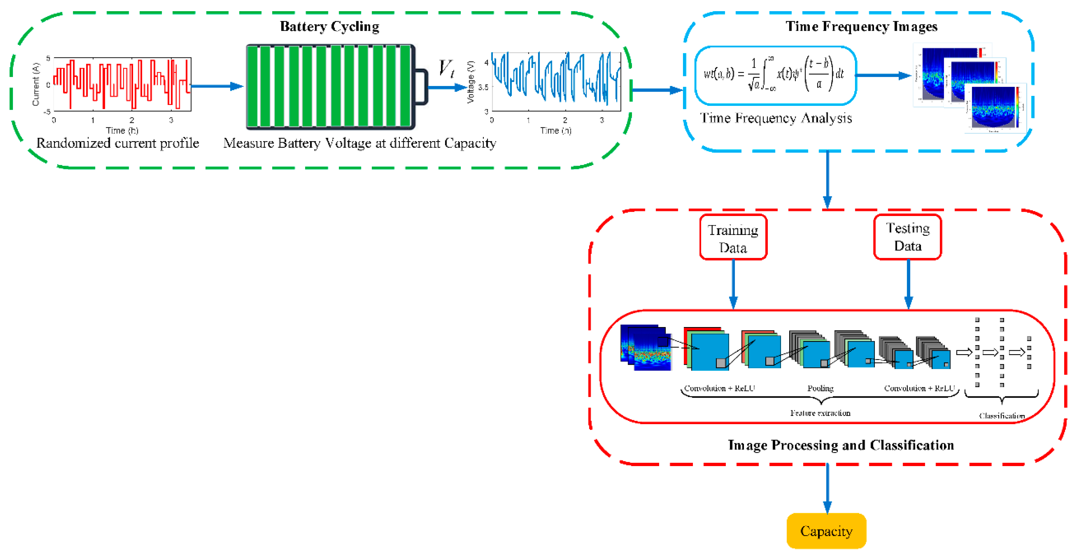
3. The Proposed Capacity Imaging Analysis Scheme

Figure 5 shows the block diagram of the proposed TFI paradigm. Here, the terminal voltage of the cycled battery using randomised current profile data is utilised to predict the capacity of the battery. Initially, the terminal voltage of the battery is measured at different capacities, and then the measured voltage is transformed from 1D raw data to a 2D time-frequency image (TFI) by applying a CWT algorithm. The raw data of the measured voltage for the LIB at different capacities contains only the time-domain information, but the converted 2D TFI features of the raw data clearly represent the time and frequency domain information at once. Finally, the generated TFIs for different battery capacities are fed into a deep learning convolutional neural network for feature extraction and image classification. The following subsections explain the capacity prediction steps in detail.

3.1. Time–Frequency Image (TFI) Analysis

The main aim of this research was the analysis and classification of the measured voltage of LIBs at different capacities using TFI analysis. As stated in Section 1, most studies have used traditional methods of time or frequency domain to analyse the LIB’s measured signals and extract diagnostic characteristics to describe the degradation inside the battery cell. Like most real-life signals, the measured LIB terminal voltage can exhibit non-stationary characteristics [31,32]. Thus, analysing the LIB’s measured voltage using traditional time or frequency domains is insufficient to extract comprehensive features about the degradation process inside the battery [39]. Nevertheless, time–frequency approaches can extract several domain features in order to assess the measured signal for the time and frequency domains, precisely extracting better features from the measured signal [40]. The main goal of a time-frequency signal processing analysis is to extract useful information features from the measured battery terminal voltage by converting the time series signal into the time–frequency domain [41,42].
Various methods can be used for time-frequency representation, such as CWT, Wigner-Ville distribution, and short-time Fourier transform (STFT). Of these, CWT is employed to transform the measured signal from the time domain to a TFI, whose energy concentrations visualise changes in frequency components over time as the battery degrades [43]. In the proposed prediction scheme, shown in Figure 5, a CWT was applied to the measured terminal voltage, to transform it from a time domain signal into a time-frequency domain scalogram image. The aim of this conversion process was to extract more useful information about the degradation process inside the battery during a randomised charging/discharging current profile. Through a set of wavelet basis functions, the wavelet transforms (WT) degraded the LIB’s terminal voltage in the time-frequency domain. This transform employed a wavelet function of a finite bandwidth in terms of the time and frequency domains. Via the scaling and translation of the wavelet basis function, the signal was degraded with various resolutions at differing scales of time and frequency [44]. Equation (3) describes the mathematical scaling and translation of basic wavelet function:
ψ a , b ( t ) =   1 a ψ ( t b a )
where ψ a ,   b ( t ) is an analysis wavelet and is called a child wavelet, a ( 0 , + ) is the scale parameter of the wavelet transform, and b ( , + ) is the translation or shift parameter in time. The function ψ ( t ) is known as the mother wavelet with finite length and fast depletion. Two limit conditions must be satisfied in the mother wavelet signal, which are ( + ψ ( t ) d t = 0   and   + | ψ ( t ) | 2 d t = 1 ) [32]. For the given time series signal x ( t ) , the wavelet coefficients w t ( a , b ) are obtained by the convolution integral of the mother wavelet ψ ( t ) and the given signal x ( t ) , as presented in (4):
w t ( a , b ) =   1 a x ( t ) ψ * ( t b a ) d t  
where ψ * means the complex conjugate of function ψ . Throughout this procedure, the signal x ( t ) is divided into a sequence of scaled and shifted wavelet coefficients, in which the wavelet set is the basis function. After this, the signal x ( t ) is altered by CWT and sent to the 2D time-frequency domains [45]. With this approach, the 1D time domain signals are transformed into TFI. Figure 6 shows an example schematic of the battery measured voltage at three different capacities and the transformed time-frequency domain representation features for each capacity. It can be observed that there are clear discriminative variations in the CWT coefficients at each capacity in the TFI. Therefore, battery degradation is well reflected by the multi-domain TFI features, which can thus be used as input for the deep learning convolutional neural network (CNN) to classify the battery’s capacity during the degradation.

3.2. Time-Frequency Image Analysis and Classification Using Deep Learning Algorithm

The obtained TFIs from the battery measured voltage at different capacities are fed into the deep learning predictive model to extract the relationship between the TFIs and corresponding capacity. In this research, a data-driven method based on transfer deep learning model is adopted to perform capacity classification in LIB.
Generally, a DL-CNN is built from three types of layers, namely (1) convolution layers, (2) pooling layers, and (3) fully connected layers [44]. The convolution and pooling layers are linked to form convolution blocks, and many of these blocks are stacked to create a deep architecture. The fully connected layer has generally been used as the final layer in the classification or regression. The general architecture of the DL-CNN is shown in Figure 7 [46].
The convolutional layer combines the input image from the initial layer with several filters, known as kernels, and these are then fed to the activation function to create a features map [47]. The output features map is the convolutional result of the input maps and can be calculated as in (5) [48]:
x j = f ( i M j x i l 1 k i j l + b j l )  
Here, ∗ is the convolutional operation, xi is ith input map, k is a F × F convolutional filter, bj is the additive bias, Mj is the feature map of the convolutional layer, and l is the lth layers in the neural network. Lastly, the obtained results from the convolutional layers are fed to the activation function. The common used activation function is the rectified linear unit (ReLU), defined as in (6) [47,48,49].
R e L U ( x ) = max ( 0 , x )
For the pooling layer, which follows the convolutional layer, low-resolution maps are created from the most significant local information. The maximum value is derived from each region by using the max pooling layer, as shown in Figure 8 [48]. In the fully connected layer, a 1D vector is utilized to represent all the feature maps, which is fully connected to the output layer. The output of the fully connected layer is described as given in (7):
O i = f ( j = 1 d x j F w i j + b i )
where O i is the output layer, x j F is the j t h neuron in the fully connected layer, w i j is the weight related to O i and x j F , b i is the bias corresponding to O i , and f is the activation function [48,50].
In this study, two deep transfer learning algorithms were applied to classify the generated results from TFI. The classification results are presented in the Results and Discussion section.

4. Results and Discussion

The proposed scheme (see Figure 5) was implemented using the MATLAB environment. First, the results of TFI estimation using complex Morlet mother wavelet transform (CMMW) will be presented in this section, and then the results of image analysis and classification using deep learning algorithms will be demonstrated.

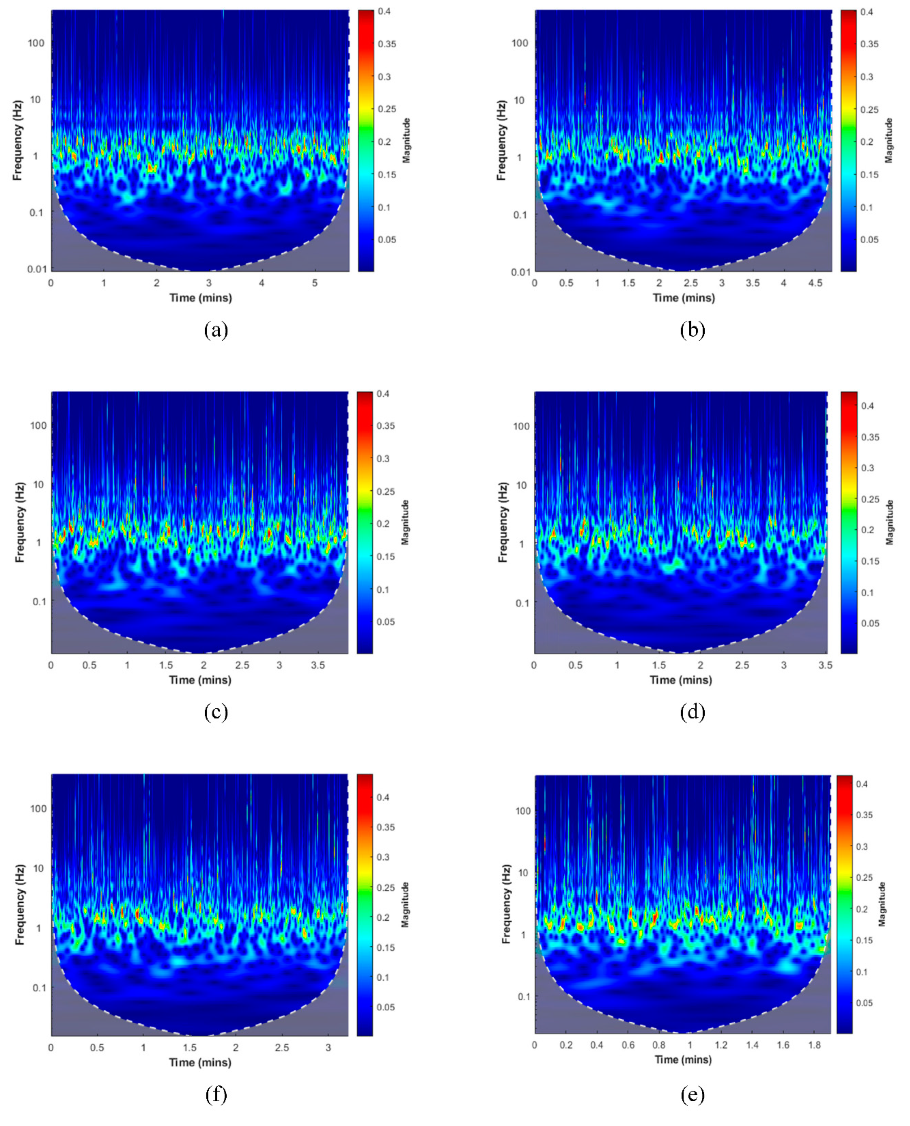
4.1. Time–Frequency Image (TFI) Results

Figure 9a shows the measured voltage signal of the first cycle of RW9 at the beginning of the life of the LIB, indicating that no degradation had occurred at this point and the battery’s capacity was full (here, C = 2.1 Ah). Figure 9c presents the measured voltage at the end of the LIB’s life and shows that the battery degraded, and its capacity decreased to its minimum value ( C = 0.8 Ah). From both results, it can be clearly observed that the battery had aged and that the time period of the measured voltage (31.07 h) at the end of life was less than that for the first cycle of the battery (93.18 h). This is because the battery has reached its threshold voltage level very frequently due to an increase in the internal resistance of the LIB, and this inherently reduces the LIB capacity.
To extract appropriate features capable of describing the degradation phenomena inside the battery from the measured voltage, CMMW was applied using Equations (3) and (4) to the LIB terminal voltage, as illustrated in Figure 9b,d. In the TFI, the energy concentration of the measured voltage of the LIB is shown at different capacities, with the horizontal and vertical axes representing time and frequency, respectively. The amplitudes of the wavelet coefficients are represented in different colours on the TFI [47]; red colour indicates that the level of energy density is high. In Figure 9b, when the LIB is at the beginning of its life, the energy distribution is concentrated in the middle frequency range of the image and varies from 1 to 2 Hz [51]. In contrast, Figure 9d shows the energy distributed in the middle and high frequency bands (up to 100 Hz) of the image, meaning that the amplitude of the wavelet coefficients increased to cover the rapid changes between the upper and lower voltage range. A comparison of the TFIs for the battery at the beginning and end of its life clearly shows a significant difference in the energy density distribution. Therefore, the capacity degradation of the battery is well reflected by the TFI information and multiple domain features can be calculated using TFI.
The datasets for the four test batteries were processed by the proposed CMMW. Figure 10 presents a sample of the results of the time-frequency images of the measured LIB terminal voltage at different capacities. They show the energy concentration distribution of the battery terminal voltage according to the level of degradation in the TFI. As shown in Figure 10, as the battery’s capacity decreases, the distribution of the energy in the TFI changes, clearly illustrating the degradation process inside the battery cell. From the extracted wavelet coefficients using CMMW, the energy concentrations for wavelet coefficients are calculated in the form of TFIs, which are then fed to the pre-trained CNN for image pattern recognition and classification.
To further validate the proposed technique, the experimental datasets of the LIBs RW10, RW11, and RW12 at different capacity ranges from 2.1 to 1.2 Ah have been tested. Table 2 demonstrates the effectiveness of the proposed TFI method to predict the capacity of these cells. Ongoing research is mainly attempting to apply the proposed technique to quantify which type of degradation mode most affects the battery’s capacity.

4.2. DL-CNN Results

In this subsection, we demonstrate how the generated TFIs from the measured terminal voltage at different capacities through CWT were fed into AlexNet and VGG-16 DL-CNNs for capacity classification, after they had been trained for TFI classification. The Stochastic gradient descent (SGDM) and adaptive moment estimation (ADAM) optimisation algorithms were used to train the generated TFIs.

4.2.1. AlexNet Neural Network

The AlexNet neural network was created in 2012 by Krizhevsky et al. [52] and is built from eight layers (five convolutional and three fully connected layers). In this study, we assumed that the battery’s capacity is classified into five classes from the first measured capacity value, which is 2.1 Ah, to the measured capacity value of 1.20 Ah in the experimental dataset—similar to the work presented in [53,54]. The measured voltage of each battery per RW cycle was labelled to show its corresponding capacity. The datasets of LIBs RW9–12 were split into training data (70% of all TFI in the four folds) and 30% for testing data. Therefore, the LIB capacity estimation can be considered a 5-class classification. The size of the generated TFIs is 227 × 227 × 3, which is suitable for the pretrained AlexNet network. The training settings for modelling the network and the AlexNet architecture are given in Table 3 and Table 4. The AlexNet output layer was replaced with a new output layer with five neurons corresponding to five classes of capacity values. Since the AlexNet network is not trained to classify TFIs, only the weights of the last convolution layer and fully connected layer were trained, while the first four convolution layers were not. Training only the last layers of the AlexNet network reduced the training time of the model [44].
During the training phase, SGDM and ADAM optimisers were utilised with an initial learning rate of 0.0001, and the batch size was set at 50. Once the training process was finished, the accuracy of the classification by the model was evaluated using the test dataset. A deep learning toolbox from MATLAB was employed to train and test the model. Classification accuracy was calculated to evaluate the model’s accuracy, and the test dataset results are given in Table 5. The results show that the trained model correctly classified the test data with an accuracy rate of 95.69%. Moreover, the SDGM and ADAM optimisers achieved good performance regarding updating the weights of our model. Thus, these classification results demonstrate that the proposed method achieved accurate predictions of battery capacity for each battery cell.

4.2.2. VGG-16 Neural Network

The second pretrained model tested in this study is a convolutional neural network from the Oxford Visual Geometry Group (VGG) which is a 16-layer network [55]. VGG-16 has achieved classification accuracy performance on the ImageNet dataset and Table 6 shows the layer structure of VGG-16. With the same hyperparameter settings, the VGG-16 model is compared with the AlexNet model and the prediction accuracy results are presented in Table 7. The comparison classification results from Table 5 and Table 7 for AlexNet and the VGG-16 models show that as the DL-CNN becomes deeper, the accuracy of the model will increase. However, as the DL-CNN becomes deeper, the training time will increase, and more computational complexity will be added to the model.

5. Conclusions

This paper proposed a new capacity evaluation method for LIBs using multi-domain features obtained from a TFI algorithm. The terminal voltage of the battery was transformed into a 2D image feature using CWT instead of 1D raw data of terminal voltage or the extraction of multiple statistical features. The proposed method was applied CWT to produce a 2D multi-domain features time–frequency representation of the battery terminal voltage, known as a TFI. To this end, experimental data on four LIBs cells published by the Prognostics Center of Excellence (PCoE) NASA were adopted to validate the effectiveness of the proposed method. The generated TF images clearly demonstrated the degradation process of the battery throughout the distribution of the energy concentration of the measured voltage for the battery at different capacity values. Two pre-trained DL-CNN were utilised to classify the generated TFIs at various capacities into five classes. The classification results achieved 95.69% accuracy using the AlexNet network and 95.52% accuracy from the VGG-16 network. The accuracy of the proposed method indicates that the proposed technique can be an effective health prognostic tool for managing LIBs for various applications such as electric vehicles and grid applications. However, the proposed method should be tested under different operating conditions (i.e., different temperatures and high-discharge current profile) to increase the accuracy of prediction and to develop a general prediction model. It is important to emphasise that the TFIs generated can be improved since the TFIs were generated by the use of a classical CWT. The resolution of the obtained energy concentration spectra affects the performance of the deep learning algorithm for capacity estimation. Our future work will therefore explore the applicability of the multi-domain features using energy concentration in time–frequency image analysis to provide robust results under different operating and temperature conditions. In addition, other time–frequency techniques such as STFT and Winger–Ville distribution will be investigated and compared to each other in terms of time–frequency resolution and computational complexity for online capacity prediction. Finally, future work will also compare computation load for the proposed algorithms.

Author Contributions

Conceptualization, M.E.-D. (Ma’d El-Dalahmeh) and M.A.-G.; methodology, M.E.-D. (Ma’d El-Dalahmeh) and M.A.-G.; formal analysis, M.E.-D. (Mo’ath El-Dalahmeh), M.A.-G., and M.E.-D. (Ma’d El-Dalahmeh); investigation, M.E.-D. (Ma’d El-Dalahmeh) and M.A.-G.; writing—original draft preparation, M.E.-D. (Mo’ath El-Dalahmeh); writing—review and editing, M.A.-G., M.S.; supervision, M.A.-G., M.S. All authors have read and agreed to the published version of the manuscript.

Funding

This research received no external funding.

Conflicts of Interest

The authors declare no conflict of interest.

References

  1. Ren, G.; Ma, G.; Cong, N. Review of electrical energy storage system for vehicular applications. Renew. Sustain. Energy Rev. 2015, 41, 225–236. [Google Scholar] [CrossRef]
  2. Waag, W.; Fleischer, C.; Sauer, D.U. Critical review of the methods for monitoring of lithium-ion batteries in electric and hybrid vehicles. J. Power Sources 2014, 258, 321–339. [Google Scholar] [CrossRef]
  3. Zhang, R.; Xia, B.; Li, B.; Cao, L.; Lai, Y.; Zheng, W.; Wang, H.; Wang, W. State of the Art of Lithium-Ion Battery SOC Estimation for Electrical Vehicles. Energies 2018, 11, 1820. [Google Scholar] [CrossRef] [Green Version]
  4. Cadini, F.; Sbarufatti, C.; Cancelliere, F.; Giglio, M. State-of-life prognosis and diagnosis of lithium-ion batteries by data-driven particle filters. Appl. Energy 2019, 235, 661–672. [Google Scholar] [CrossRef]
  5. Vetter, J.; Novák, P.; Wagner, M.R.; Veit, C.; Möller, K.C.; Besenhard, J.O.; Winter, M.; Wohlfahrt-Mehrens, M.; Vogler, C.; Hammouche, A. Ageing mechanisms in lithium-ion batteries. J. Power Sources 2005, 147, 269–281. [Google Scholar] [CrossRef]
  6. Lu, L.; Han, X.; Li, J.; Hua, J.; Ouyang, M. A review on the key issues for lithium-ion battery management in electric vehicles. J. Power Sources 2013, 226, 272–288. [Google Scholar] [CrossRef]
  7. Farmann, A.; Waag, W.; Marongiu, A.; Sauer, D.U. Critical review of on-board capacity estimation techniques for lithium-ion batteries in electric and hybrid electric vehicles. J. Power Sources 2015, 281, 114–130. [Google Scholar] [CrossRef]
  8. Tian, H.; Qin, P.; Li, K.; Zhao, Z. A review of the state of health for lithium-ion batteries: Research status and suggestions. J. Clean. Prod. 2020, 261, 120813. [Google Scholar] [CrossRef]
  9. Berecibar, M.; Gandiaga, I.; Villarreal, I.; Omar, N.; Van Mierlo, J.; Van den Bossche, P. Critical review of state of health estimation methods of Li-ion batteries for real applications. Renew. Sustain. Energy Rev. 2016, 56, 572–587. [Google Scholar] [CrossRef]
  10. Lipu, M.S.H.; Hannan, M.A.; Hussain, A.; Hoque, M.M.; Ker, P.J.; Saad, M.H.M.; Ayob, A. A review of state of health and remaining useful life estimation methods for lithium-ion battery in electric vehicles: Challenges and recommendations. J. Clean. Prod. 2018, 205, 115–133. [Google Scholar] [CrossRef]
  11. Xiong, R.; Li, L.; Tian, J. Towards a smarter battery management system: A critical review on battery state of health monitoring methods. J. Power Sources 2018, 405, 18–29. [Google Scholar] [CrossRef]
  12. Meng, H.; Li, Y.-F. A review on prognostics and health management (PHM) methods of lithium-ion batteries. Renew. Sustain. Energy Rev. 2019, 116, 109405. [Google Scholar] [CrossRef]
  13. Plett, G.L. Extended Kalman filtering for battery management systems of LiPB-based HEV battery packs: Part 3. State and parameter estimation. J. Power Sources 2004, 134, 277–292. [Google Scholar] [CrossRef]
  14. Bian, X.; Liu, L.; Yan, J. A model for state-of-health estimation of lithium ion batteries based on charging profiles. Energy 2019, 177, 57–65. [Google Scholar] [CrossRef]
  15. Zou, Y.; Hu, X.; Ma, H.; Li, S.E. Combined State of Charge and State of Health estimation over lithium-ion battery cell cycle lifespan for electric vehicles. J. Power Sources 2015, 273, 793–803. [Google Scholar] [CrossRef]
  16. Bartlett, A.; Marcicki, J.; Onori, S.; Rizzoni, G.; Yang, X.G.; Miller, T. Electrochemical Model-Based State of Charge and Capacity Estimation for a Composite Electrode Lithium-Ion Battery. IEEE Trans. Control Syst. Technol. 2016, 24, 384–399. [Google Scholar] [CrossRef]
  17. Lotfi, N.; Li, J.; Landers, R.G.; Park, J. Li-ion Battery State of Health Estimation based on an improved Single Particle model. In Proceedings of the 2017 American Control Conference (ACC), Seattle, WA, USA, 24–26 May 2017; pp. 86–91. [Google Scholar]
  18. Wu, B.; Han, S.; Shin, K.G.; Lu, W. Application of artificial neural networks in design of lithium-ion batteries. J. Power Sources 2018, 395, 128–136. [Google Scholar] [CrossRef]
  19. Hu, C.; Jain, G.; Zhang, P.; Schmidt, C.; Gomadam, P.; Gorka, T. Data-driven method based on particle swarm optimization and k-nearest neighbor regression for estimating capacity of lithium-ion battery. Appl. Energy 2014, 129, 49–55. [Google Scholar] [CrossRef]
  20. Hu, X.; Li, S.; Peng, H. A comparative study of equivalent circuit models for Li-ion batteries. J. Power Sources 2012, 198, 359–367. [Google Scholar] [CrossRef]
  21. Li, J.; Adewuyi, K.; Lotfi, N.; Landers, R.G.; Park, J. A single particle model with chemical/mechanical degradation physics for lithium ion battery State of Health (SOH) estimation. Appl. Energy 2018, 212, 1178–1190. [Google Scholar] [CrossRef]
  22. Lin, C.; Xing, J.; Tang, A. Lithium-ion Battery State of Charge/State of Health Estimation Using SMO for EVs. Energy Procedia 2017, 105, 4383–4388. [Google Scholar] [CrossRef]
  23. Li, Y.; Liu, K.; Foley, A.M.; Zülke, A.; Berecibar, M.; Nanini-Maury, E.; Van Mierlo, J.; Hoster, H.E. Data-driven health estimation and lifetime prediction of lithium-ion batteries: A review. Renew. Sustain. Energy Rev. 2019, 113, 109254. [Google Scholar] [CrossRef]
  24. Ng, M.-F.; Zhao, J.; Yan, Q.; Conduit, G.J.; Seh, Z.W. Predicting the state of charge and health of batteries using data-driven machine learning. Nat. Mach. Intell. 2020, 2, 161–170. [Google Scholar] [CrossRef] [Green Version]
  25. Nuhic, A.; Terzimehic, T.; Soczka-Guth, T.; Buchholz, M.; Dietmayer, K. Health diagnosis and remaining useful life prognostics of lithium-ion batteries using data-driven methods. J. Power Sources 2013, 239, 680–688. [Google Scholar] [CrossRef]
  26. Severson, K.A.; Attia, P.M.; Jin, N.; Perkins, N.; Jiang, B.; Yang, Z.; Chen, M.H.; Aykol, M.; Herring, P.K.; Fraggedakis, D.; et al. Data-driven prediction of battery cycle life before capacity degradation. Nat. Energy 2019, 4, 383–391. [Google Scholar] [CrossRef] [Green Version]
  27. Pan, H.; Lü, Z.; Wang, H.; Wei, H.; Chen, L. Novel battery state-of-health online estimation method using multiple health indicators and an extreme learning machine. Energy 2018, 160, 466–477. [Google Scholar] [CrossRef]
  28. Hu, C.; Jain, G.; Schmidt, C.; Strief, C.; Sullivan, M. Online estimation of lithium-ion battery capacity using sparse Bayesian learning. J. Power Sources 2015, 289, 105–113. [Google Scholar] [CrossRef]
  29. Venugopal, P.; Vigneswaran, T. State-of-Health Estimation of Li-ion Batteries in Electric Vehicle Using IndRNN under Variable Load Condition. Energies 2019, 12, 4338. [Google Scholar] [CrossRef] [Green Version]
  30. Khaleghi, S.; Firouz, Y.; Van Mierlo, J.; Van den Bossche, P. Developing a real-time data-driven battery health diagnosis method, using time and frequency domain condition indicators. Appl. Energy 2019, 255, 113813. [Google Scholar] [CrossRef]
  31. Kim, J. Discrete Wavelet Transform-Based Feature Extraction of Experimental Voltage Signal for Li-Ion Cell Consistency. IEEE Trans. Veh. Technol. 2016, 65, 1150–1161. [Google Scholar] [CrossRef]
  32. Cai, Y.; Yang, L.; Deng, Z.; Zhao, X.; Deng, H. Online identification of lithium-ion battery state-of-health based on fast wavelet transform and cross D-Markov machine. Energy 2018, 147, 621–635. [Google Scholar] [CrossRef]
  33. You, G.-W.; Park, S.; Oh, D. Real-time state-of-health estimation for electric vehicle batteries: A data-driven approach. Appl. Energy 2016, 176, 92–103. [Google Scholar] [CrossRef]
  34. Shen, S.; Sadoughi, M.; Chen, X.; Hong, M.; Hu, C. A deep learning method for online capacity estimation of lithium-ion batteries. J. Energy Storage 2019, 25, 100817. [Google Scholar] [CrossRef]
  35. Shen, S.; Sadoughi, M.; Li, M.; Wang, Z.; Hu, C. Deep convolutional neural networks with ensemble learning and transfer learning for capacity estimation of lithium-ion batteries. Appl. Energy 2020, 260, 114296. [Google Scholar] [CrossRef]
  36. Bole, B.; Kulkarni, C.S.; Daigle, M. Randomized battery usage data set. NASA AMES Progn. Data Repos. 2014, 70. Available online: https://ti.arc.nasa.gov/tech/dash/groups/pcoe/prognostic-data-repository/ (accessed on 10 October 2020).
  37. Bole, B.; Kulkarni, C.S.; Daigle, M. Adaptation of an electrochemistry-based Li-ion battery model to account for deterioration observed under randomized use. Proc. Annu. Conf. Progn. Health Manag. Soc. 2014, 2, 1–9. [Google Scholar]
  38. Yu, J.; Mo, B.; Tang, D.; Yang, J.; Wan, J.; Liu, J. Indirect State-of-Health Estimation for Lithium-Ion Batteries under Randomized Use. Energies 2017, 10, 2012. [Google Scholar] [CrossRef] [Green Version]
  39. Feltane, A. Time-Frequency Based Methods for Non-Stationary Signal Analysis with Application To EEG Signals. Ph.D. Thesis, The University of Rhode Island, Kingston, RL, USA, 2016. [Google Scholar]
  40. Sejdić, E.; Orović, I.; Stanković, S. Compressive sensing meets time–frequency: An overview of recent advances in time–frequency processing of sparse signals. Digit. Signal Process. 2018, 77, 22–35. [Google Scholar] [CrossRef]
  41. Li, X.; Ding, Q.; Sun, J.-Q. Remaining useful life estimation in prognostics using deep convolution neural networks. Reliab. Eng. Syst. Saf. 2018, 172, 1–11. [Google Scholar] [CrossRef] [Green Version]
  42. Boashash, B.; Ouelha, S. Automatic signal abnormality detection using time-frequency features and machine learning: A newborn EEG seizure case study. Knowl. Based Syst. 2016, 106, 38–50. [Google Scholar] [CrossRef]
  43. Yan, R.; Gao, R.X.; Chen, X. Wavelets for fault diagnosis of rotary machines: A review with applications. Signal Process. 2014, 96, 1–15. [Google Scholar] [CrossRef]
  44. Shao, S.; McAleer, S.; Yan, R.; Baldi, P. Highly Accurate Machine Fault Diagnosis Using Deep Transfer Learning. IEEE Trans. Ind. Inform. 2019, 15, 2446–2455. [Google Scholar] [CrossRef]
  45. Boashash, B.; Ouelha, S. Designing high-resolution time–frequency and time–scale distributions for the analysis and classification of non-stationary signals: A tutorial review with a comparison of features performance. Digit. Signal Process. 2018, 77, 120–152. [Google Scholar] [CrossRef]
  46. Nielsen, M.A. Neural Networks and Deep Learning; Determination press: San Francisco, CA, USA, 2015; Volume 2018. [Google Scholar]
  47. Yoo, Y.; Baek, J.-G. A Novel Image Feature for the Remaining Useful Lifetime Prediction of Bearings Based on Continuous Wavelet Transform and Convolutional Neural Network. Appl. Sci. 2018, 8, 1102. [Google Scholar] [CrossRef] [Green Version]
  48. Schmidhuber, J. Deep learning in neural networks: An overview. Neural Netw. 2015, 61, 85–117. [Google Scholar] [CrossRef] [Green Version]
  49. Aggarwal, C.C. Neural Networks and Deep Learning; Springer: Cham, Switzerland, 2018. [Google Scholar]
  50. Liao, Y.; Zeng, X.; Li, W. Wavelet transform based convolutional neural network for gearbox fault classification. In Proceedings of the 2017 Prognostics and System Health Management Conference (PHM-Harbin), Harbin, China, 9–12 July 2017; pp. 1–6. [Google Scholar]
  51. Zhang, Y.; Tang, Q.; Zhang, Y.; Wang, J.; Stimming, U.; Lee, A.A. Identifying degradation patterns of lithium ion batteries from impedance spectroscopy using machine learning. Nat. Commun. 2020, 11, 1706. [Google Scholar] [CrossRef] [PubMed]
  52. Krizhevsky, A.; Sutskever, I.; Hinton, G.E. Imagenet classification with deep convolutional neural networks. In Proceedings of the Advances in Neural Information Processing Systems 25 (NIPS 2012), Lake Tahoe, NV, USA, 3–8 December 2012; pp. 1097–1105. [Google Scholar]
  53. Patil, M.A.; Tagade, P.; Hariharan, K.S.; Kolake, S.M.; Song, T.; Yeo, T.; Doo, S. A novel multistage Support Vector Machine based approach for Li ion battery remaining useful life estimation. Appl. Energy 2015, 159, 285–297. [Google Scholar] [CrossRef]
  54. Ali, M.U.; Zafar, A.; Nengroo, S.H.; Hussain, S.; Park, G.-S.; Kim, H.-J. Online Remaining Useful Life Prediction for Lithium-Ion Batteries Using Partial Discharge Data Features. Energies 2019, 12, 4366. [Google Scholar] [CrossRef] [Green Version]
  55. Simonyan, K.; Zisserman, A. Very deep convolutional networks for large-scale image recognition. arXiv 2014, arXiv:1409.1556. [Google Scholar]
Figure 1. The cycle processes.
Energies 13 05447 g001
Figure 2. Voltage, current, and temperature of the first 100 steps measured for battery RW9.
Energies 13 05447 g002
Figure 3. Voltage, current, and temperature of the last 100 steps measured for battery RW9.
Energies 13 05447 g003
Figure 4. Capacities of the measured cells for four batteries, RW9, RW10, RW11, and RW12.
Energies 13 05447 g004
Figure 5. General flow chart of the proposed method for TFI capacity estimation.
Energies 13 05447 g005
Figure 6. Measured voltage of lithium-ion battery and transformed TFI energy concentration spectrum information of the measured voltage at three different capacity values.
Energies 13 05447 g006
Figure 7. Deep learning convolutional neural network architecture.
Energies 13 05447 g007
Figure 8. Max pooling layer.
Energies 13 05447 g008
Figure 9. Time-domain measured voltage and plot of TFI energy concentration spectrum of battery cell (RW9): (a) measured voltage signal (beginning of life), (b) wavelet energy concentration spectrum (beginning of life), (c) measured voltage signal (end of life), and (d) wavelet energy concentration spectrum (end of life).
Energies 13 05447 g009
Figure 10. TFI energy concentration spectrum results of the battery RW9 measured voltage at different capacities: (a) 2.1, (b) 1.8, (c) 1.6, (d) 1.4, (f) 1.2, (e) 0.8 Ah.
Energies 13 05447 g010
Table 1. The general characteristics of the tested cells.
Battery Properties18650 LIBs
ManufactureLG Chem
Chemistry18650 lithium cobalt oxide vs. graphite
Nominal capacity2.10 Ah
Capacity range2.10 Ah–0.80 Ah
Voltage range4.2–3.2 V
Table 2. TFIs energy concentration spectrum results of RW10, RW11, and RW12 LIBs measured voltage at different capacities.
Capacity (Ah)RW10RW11RW12
2.1 Energies 13 05447 i001 Energies 13 05447 i002 Energies 13 05447 i003
1.8 Energies 13 05447 i004 Energies 13 05447 i005 Energies 13 05447 i006
1.6 Energies 13 05447 i007 Energies 13 05447 i008 Energies 13 05447 i009
1.4 Energies 13 05447 i010 Energies 13 05447 i011 Energies 13 05447 i012
1.2 Energies 13 05447 i013 Energies 13 05447 i014 Energies 13 05447 i015
Table 3. Hyperparameter settings for the trained AlexNet model.
HyperparametersValues
Momentum0.9
Initial learning rate0.0001
Learning rate drop factor0.1
Learning rate drop period10
Number of epochs50
Batch size15
OptimiserSGDM, ADAM
Table 4. AlexNet architecture.
NameTypeActivationsLearnable
Data 227 × 227 × 3 imagesImage input227 × 227 × 3-
Conv 1Convolution55 × 55 × 96Weights 11 × 11 × 3 × 96 Bias 1 × 1 × 96
Pool 1Max Pooling27 × 27 × 96-
Conv 2Convolution27 × 27 × 256Weights 5 × 5 × 48 × 256 Bias 1 × 1x256
Pool 2Max Pooling13 × 13 × 256-
Conv 3Convolution13 × 13 × 384Weights 3 × 3 × 256 × 384 Bias 1 × 1 × 384
Conv 4Convolution13 × 13 × 384Weights 3 × 3 × 192 × 384 Bias 1 × 1 × 384
Conv 5Convolution13 × 13 × 256Weights 3 × 3 × 192 × 256 Bias 1 × 1x256
Pool 5Max Pooling6 × 6 × 256-
Fc6Fully Connected1 × 1 × 4096Weights 4096 × 9216 Bias 4096 × 1
Fc7Fully Connected1 × 1 × 4096Weights 4096 × 4096 Bias 4096 × 1
Fc8Fully Connected1 × 1 × 1000Weights 1000 × 4096 Bias 1000 × 1
Prob Softmax layerSoftmax1 × 1 × 1000-
OutputClassification--
Table 5. Capacity prediction accuracy for each battery cell using AlexNet.
RW9RW10RW11RW12
OptimiserSGDMAdamSGDMADAMSGDMADAMSGDMADAM
Accuracy95.0673%95.69%91.96%94.20%93.39%94.27%90.25%91.5%
Table 6. VGG-16 architecture hyperparameters.
NameTypeActivationsLearnable
Data 224 × 224 × 3 imagesImage input224 × 224 × 3-
Block 1-Conv 1Convolution224 × 224 × 64Weights 3 × 3 × 3 × 64, Bias 1 × 1x 64
Block 1-Conv 2Convolution224 × 224 × 64Weights 3 × 3 × 3 × 64, Bias 1 × 1 × 64
Block 1-PoolMax Pooling112 × 112 × 64-
Block 2-Conv 1Convolution112 × 112 × 128Weights 3 × 3 × 64 × 128, Bias 1 × 1 × 128
Block 2-Conv 2Convolution112 × 112 × 128Weights 3 × 3 × 128 × 128, Bias 1 × 1 × 128
Block 2-PoolMax Pooling56 × 56 × 128-
Block 3-Conv 1Convolution56 × 56 × 256Weights 3 × 3 × 128 × 256, Bias 1 × 1 × 256
Block 3-Conv 2Convolution56 × 56 × 256Weights 3 × 3 × 128 × 256, Bias 1 × 1 × 256
Block 3-PoolMax Pooling28 × 28 × 256-
Block 4-Conv 1Convolution28 × 28 × 512Weights 3 × 3 × 256 × 512, Bias 1 × 1 × 512
Block 4-Conv 2Convolution28 × 28 × 512Weights 3 × 3 × 256 × 512, Bias 1 × 1 × 512
Block 4-PoolMax Pooling14 × 14 × 512-
Block 5-Conv 1Convolution14 × 14 × 512Weights 3 × 3 × 512 × 512, Bias 1 × 1 × 512
Block 5-Conv 2Convolution14 × 14 × 512Weights 3 × 3 × 512 × 512, Bias 1 × 1 × 512
Block 5-PoolMax Pooling7 × 7 × 512-
Fc1Fully Connected1 × 1 × 4096Weights 4096 × 4096, Bias 4096 × 1
Fc2Fully Connected1 × 1 × 4096Weights 4096 × 4096, Bias 4096 × 1
Prob Softmax layerSoftmax1 × 1 × 1000-
OutputClassification --
Table 7. Capacity prediction accuracy for each battery cell using the VGG-16 model.
RW9RW10RW11RW12
OptimiserSGDMADAMSGDMADAMSGDMADAMSGDMADAM
Accuracy95.52%95.52%95.09%95.60%94.29%94.92%92.25%95.5%
Publisher’s Note: MDPI stays neutral with regard to jurisdictional claims in published maps and institutional affiliations.

