Article

An All-At-Once Newton Strategy for Marine Methane Hydrate Reservoir Models

by
Shubhangi Gupta
1,2,*,
Barbara Wohlmuth
2 and
Matthias Haeckel
1
1
GEOMAR Helmholtz Center for Ocean Research Kiel, Wischhofstraße 1-3, 24148 Kiel, Germany
2
Department of Mathematics, Technical University of Munich, Boltzmannstraße 3, 85748 Garching bei München, Germany
*
Author to whom correspondence should be addressed.
Energies 2020, 13(2), 503; https://doi.org/10.3390/en13020503
Submission received: 13 December 2019 / Revised: 13 January 2020 / Accepted: 14 January 2020 / Published: 20 January 2020
(This article belongs to the Special Issue Advances in Natural Gas Hydrates)

Abstract

:
The migration of methane through the gas hydrate stability zone (GHSZ) in the marine subsurface is characterized by highly dynamic reactive transport processes coupled to thermodynamic phase transitions between solid gas hydrates, free methane gas, and dissolved methane in the aqueous phase. The marine subsurface is essentially a water-saturated porous medium where the thermodynamic instability of the hydrate phase can cause free gas pockets to appear and disappear locally, causing the model to degenerate. This poses serious convergence issues for the general-purpose nonlinear solvers (e.g., standard Newton), and often leads to extremely small time-step sizes. The convergence problem is particularly severe when the rate of hydrate phase change is much lower than the rate of gas dissolution. In order to overcome this numerical challenge, we have developed an all-at-once Newton scheme tailored to our gas hydrate model, which can handle rate-based hydrate phase change coupled with equilibrium gas dissolution in a mathematically consistent and robust manner.

1. Introduction

Methane hydrates constitute a dominant organic carbon pool in the Earth system, and an important intermediate “capacitor” in the global methane budget. Gas hydrates (gas hydrates and methane hydrates are used interchangeably, as in the settings of our interest gas hydrates are predominantly composed of methane; the contribution of other gases is negligible) are predominantly formed from biogenic methane generated by the microbial degradation of organic matter (methanogenesis) in the deep biosphere. This methane migrates upwards as free gas or methane-rich porewater by advection. This fluid flow is caused by non-steady-state sediment compaction (passive margins), the compaction of oceanic sediments during subduction (active margins), and the dewatering of minerals at elevated temperatures (passive + active margins). Over geological time, the hydrates accumulate close to the bottom simulation reflector (BSR, the lower stability limit of gas hydrates) because the methane flux from below leads to hydrate formation in the gas hydrate stability zone (GHSZ). However, the ongoing sedimentation tends to bury the hydrates below the GHSZ where the hydrates dissociate, and the released methane gas migrates back into the GHSZ to re-form the hydrates. Towards the seafloor, the hydrates dissolve due to undersaturation of porewaters as a consequence of the anaerobic oxidation of methane (AOM). Some methane gas by-passes the GHSZ and AOM zone if the upward flow is larger than the reaction rates. This methane fuels rich cold seep ecosystems [1]. One of our main motivations for modeling methane hydrate geosystems is to understand the role of gas migration through the GHSZ in the natural carbon cycle [2]. Methane hydrates are also seen as an attractive future energy resource. It is estimated that the total carbon content of gas hydrates is possibly larger than the combined carbon content of all other fossil fuels [3,4,5]. However, there are a number of serious environmental risks associated with the exploitation of gas hydrate reservoirs for the purpose of gas production, such as methane leakage and related global warming, ecological hazards, and geomechanical and structural instabilities [6,7]. Therefore, we also apply our gas hydrate models for feasibility analysis and risk assessment of various gas production scenarios. It is therefore evident that we require our gas hydrate models to be robust and stable across a range of spatial and temporal scales.
One of the main challenges in modeling methane hydrate geosystems comes from the complex phase transitions which cause phases to appear and disappear locally. For example, when methane hydrates dissociate due to changes in the local thermodynamic state (i.e., temperature, pressure, and salinity), they release methane and water. Methane is released as microscopic gas bubbles which, depending on the local solubility limit for methane dissolution, either collapse into the water phase or coalesce, leading to the appearance a free gas phase. Conversely, when methane hydrates form, given the right temperature, pressure, and salinity conditions, they consume methane, which may lead to the disappearance of the free gas phase. In multiphase multicomponent models, the appearance or disappearance of phases causes the model to degenerate, such that the Jacobian becomes locally indeterminate [8,9]. For methane hydrate models in particular, additional numerical challenges arise. Firstly, the hydrate and gaseous-aqueous phase transitions are strongly coupled through nonlinear mass and thermal source and sink terms which are highly sensitive to the local thermodynamic state. Even a small change in temperature, pressure, or salinity (e.g., due to climate change, sedimentation, etc.) can locally destabilize hydrates and result in a free gas pocket with lower salinity (due to the release of fresh water bound to the hydrates), lower temperature (due to exothermic hydrate dissociation), and elevated pore pressure (due to the release of a large volume of gas). These temperature, pressure, and salinity changes may in turn push the hydrates back into the stability zone. It is therefore very difficult to determine the local phase states. Secondly, for the problems at geological scales, the rate of hydrate phase change is often several orders of magnitude lower compared to the rate of methane dissolution. This difference in the rates of the phase changes makes it even harder to determine the local phase states consistently.
A variety of numerical methods have been developed to handle the phase transitions in porous media models, such as primary variable switching (PVS) schemes [10,11], the method of negative saturations [12], the method of persistent variables [13,14], and semi-smooth Newton approaches [15,16,17,18]. In the most widely used gas hydrate reservoir simulators (e.g., TOUGH-Hydrate [19], HYRES-C [20,21], STOMP-HYD [22], HRS [23,24], including our own models [25]), the gaseous–aqueous phase transitions are handled using the PVS schemes, where the choice of the primary variables is adapted locally to the phase state. This method is conceptually relatively simple and works well for oil and gas reservoir models. However, in gas hydrate models, the phase states tend to switch back and forth rapidly due to the strong coupling and nonlinearities, which often leads to spurious oscillations and a drastic reduction in time-step size, and in the extreme case, even to a breakdown of the numerical algorithm. Some gas hydrate models (e.g., [26,27], based on Code_Bright) use the method of persistent variables. This method is more stable than PVS in general, but for gas hydrate models it can be somewhat limiting because the capillary pressure relationships for hydrate-bearing sediments are very complex functions of not only the water saturation, but also the hydrate saturation (and possibly, the porosity as well as ice saturation), and therefore some parameterizations for capillary pressure may not be easy to invert, or in extreme cases, capillary pressure may not be invertible at all (e.g., experimental measure fields).
In this article, we present a robust implicit semi-smooth Newton scheme based on an NCP approach for handling the phase transitions in our methane hydrate model which includes rate-based hydrate phase change coupled with the vapor–liquid equilibrium across the gas–water interface. The advantage of an NCP approach is that it ensures that the primary variables of our mathematical model remain the same throughout the simulation, and that the constraints are realized in a variationally consistent manner, resulting in a more robust numerical scheme. As a general outline, we cast the inequality constraints arising from the vapor–liquid-equilibrium (VLE) assumption (e.g., [28]) for the C H 4 H 2 O system into a set of complementarity conditions which lead to the mathematical structure of a variational inequality (e.g., [29,30]). We reformulate the complementarity conditions as a set of non-differentiable but semi-smooth functions which are solved together with the governing PDEs of the methane hydrate model fully implicitly using a semi-smooth Newton method (e.g., [31] and the references therein). We implement our semi-smooth Newton method using an active-set strategy (e.g., [32,33]), where the Jacobian is uniquely determined based on the local phase states which are partitioned into active/inactive sets using the semi-smooth NCP functions.

2. Mathematical Model

Here, we introduce our complete mathematical model for methane hydrates in the marine subsurface (extended from [25]). The model is founded on the theory of porous media on the continuum scale. The representative elementary volume (REV) underlying the model is shown in Figure 1.
The model considers two fluid phases: gaseous and aqueous; and two solid phases: porous granular material (sediment) and methane hydrate. The sediment phase is referred to as the primary matrix, the hydrate + sediment as the composite matrix, and the fluid and the hydrate phases together as the pore-filling phases The phases are identified with the subscripts g, w, s, and h, respectively. The sediment is assumed to be perfectly rigid (geomechanics is ignored within the scope of this work). The fluid phases are mobile, while the hydrate phase is assumed immobile. Methane hydrate phase change is modeled as a kinetic reaction which is strongly dependent on the local thermodynamic state of the system. The hydrate phase is assumed to contain only pure methane hydrate. Gas adsorption/desorption on the surface of hydrates is not considered. In marine settings, water salinity has a strong influence on the thermodynamics and phase transitions. Therefore, the model also considers the transport of dissolved salts. The miscibility of methane is also accounted for. Therefore, in our model the gaseous phase is comprised of two components: methane and water. Meanwhile, the aqueous phase is comprised of three components: methane, water, and salts. The components are identified by the superscripts C H 4 , H 2 O , and c, for methane, water, and salts, respectively. The model also accounts for the thermal effects, especially the volumetric heat generation due to hydrate phase change, but assumes a local thermal equilibrium within an REV, such that a single average temperature can be defined over an REV.
In the subsequent text, the following notation is used: Subscript “ α = g , w ” denotes the fluid phases, “ β = g , w , h ” denotes the pore-filling phases, and the superscript “ κ = C H 4 , H 2 O , c ” denotes the components. Phase saturations are denoted with S β , and mole fractions of each component κ in each fluid phase α are denoted with χ α κ . Note that χ g c = 0 . Fluid phase pressures are denoted with P α , temperature is denoted with T, and porosity is denoted with ϕ ( ϕ refers to the total porosity, which indicates the void spaces within the primary sediment matrix. This is different from apparent porosity ϕ e f f , which indicates the actual void spaces available for the fluid flow. See Figure 1 for more details).

2.1. Governing Equations

2.1.1. Mass, Momentum, and Energy Conservation

The transport processes characterizing the gas production from sub-surface methane hydrate reservoir are described by invoking the conservation laws for mass, momentum, and energy described for the macroscale properties of the porous medium derived using local volume averaging principles [34,35,36]. Mass balance is considered component-wise for each κ = C H 4 , H 2 O ,
α t ϕ ρ α χ α κ S α + α · ρ α χ α κ v α = α · ϕ S α J α κ + g ˙ κ ,
where v α denotes the velocity of the fluid phase α relative to the primary sediment matrix, and J α κ denotes the diffusive flux of the component κ in the phase α . Mass balance for the hydrate phase is given by
t ϕ ρ h S h = g ˙ h .
The terms g ˙ C H 4 , g ˙ H 2 O , and g ˙ h denote the volumetric source terms resulting from the hydrate phase change, s.t., g ˙ C H 4 + g ˙ H 2 O + g ˙ h = 0 . Mass balance for the dissolved salt is given by
t ϕ ρ w S w χ w c + · ρ w χ w c v w = · ϕ S w J w c ,
where J w c is the Fickian diffusion flux of salt in the aqueous phase. Momentum balance for the fluid phases can be reduced to Darcy’s Law (e.g., [28]),
v α = K k r α μ α P α ρ α g ,
where K denotes the intrinsic permeability of the composite matrix, k r α denotes the relative permeabilities, and μ α the dynamic viscosities. The primary matrix is assumed rigid and the hydrate phase is assumed immobile. Therefore, the momentum of the solid phases is always conserved. For describing the energy conservation in the porous medium, one energy balance equation is sufficient since local thermal equilibrium has been assumed (e.g., [28]). The energy balance is given by
t 1 ϕ ρ s u s + β ϕ S β ρ β u β + α · ρ α v α h α = · k e f f t h T + Q ˙ h ,
where Q ˙ h denotes the heat of hydrate phase change. The term h α is the specific enthalpy of fluid phase α , u γ is the specific internal energy of any phase γ = g , w , h , s , and k e f f t h is the effective (or lumped) thermal conductivity, s.t.
h α = T r e f T C p α d T , u γ = T r e f T C v γ d T , and , k e f f t h = 1 ϕ k s t h + β ϕ S β k β t h .

2.1.2. Closure Relationships

The phase saturations and the phase pressures are not independent. The saturations of the pore-filling phases are related through the summation condition,
β S β = 1 .
The pressures of the fluid phases are related through a capillary pressure P c as
P g P w = P c ( S w , S h , ϕ ) .
This pressure difference occurs across the gaseous and aqueous phase interface due to balancing of cohesive forces within the liquid and the adhesive forces between the liquid and soil matrix. The parametrization used for approximating P c is discussed in Section 2.2.4.

2.2. Constitutive Relations

The nine governing Equations (1)–(7) consist of the following 25 unknowns:
S β , χ α κ , P α , P c , T , v α , J α κ , g ˙ C H 4 , g ˙ H 2 O , g ˙ h , Q ˙ h .
To close the model, we define 16 additional constitutive relationships in this section for the unknowns χ α κ , J α κ , P c , g ˙ C H 4 , g ˙ H 2 O , g ˙ h , and Q ˙ h . Some other properties which are important for modelling hydrate geosystems are also discussed.

2.2.1. Vapor–Liquid Equilibrium

Methane and water components are assumed to exist in a state of vapor–liquid equilibrium (VLE), and Henry’s law and the Raoult’s law are assumed to be valid:
Henry s law , z C H 4 χ g C H 4 P g = H w C H 4 χ w C H 4 ,
Raoult s law , χ g H 2 O P g = P s a t H 2 O χ w H 2 O ,
where z C H 4 is the methane gas compressibility, H w C H 4 is the pressure-corrected Henry’s law solubility constant for methane dissolution in water, and P s a t H 2 O is the saturation vapor pressure for water in contact with methane gas. In addition to relationships (8) and (9), we observe that within each phase α , the sum of the constituent mole fractions is bounded from above by one, and the equality holds only if the phase is present:
κ χ α κ 1 α and κ χ α κ = 1 iff S α > 0 .
We can cast the conditions in (10) as a set of Kharush–Kuhn–Tucker complementarity conditions [37] as
1 κ χ α κ 1 , S α 0 , S α 1 κ χ α κ = 0 , α .

2.2.2. Diffusive Mass Flux

The diffusive solute flux through the composite sediment matrix is evaluated using Fick’s Law (e.g., [28]),
J α κ = τ D α κ ρ α χ α κ ,
where τ denotes the tortuosity of the composite sediment matrix, and D α κ are the molecular diffusion coefficients for components κ through fluid phases α . Additionally, the summation conditions κ J α κ = 0 hold for all phases α . Note that J g c = 0 since χ g c = 0 .

2.2.3. Hydrate Phase Change Kinetics

When solid methane hydrates are warmed or depressurized, they decompose into methane gas and liquid water, and vice versa. This chemical reaction is expressed as C H 4 · N h H 2 O C H 4 + N h H 2 O , where N h gives the stoichiometry of water molecules per molecule of gas (i.e., the hydration number). The rate of this reaction is modeled by the Kim–Bishnoi kinetic model [38], where the rate of methane and water generated as a result of hydrate phase change are evaluated as
g ˙ C H 4 = k r M C H 4 A r s P e P g ,
g ˙ H 2 O = g ˙ C H 4 N h M H 2 O M C H 4 ,
where P e is the equilibrium pressure for the methane hydrate, k r is the kinetic rate constant, and A r s is the specific reaction surface area. Note that if P e P g > 0 , the hydrate becomes unstable. In this case k r refers to the dissociation rate constant. Alternatively, if P e P g < 0 , the hydrate becomes stable. In this case, k r refers to the formation rate constant. M κ denotes the molar weights, and for methane hydrate, M h = M C H 4 + N h M H 2 O . Additionally, the following condition holds:
g ˙ C H 4 + g ˙ H 2 O + g ˙ h = 0 .
For the hydrate phase change, the following constraints are considered: Hydrate dissociation can occur only when hydrate is available and the gas phase pressure is lower than the hydrate equilibrium pressure, and conversely, hydrate formation can occur only when both water and gaseous methane are available and the gas pressure is higher than the hydrate equilibrium pressure:
g ˙ h < 0 iff P g < P e and S h > 0 ,
and , g ˙ h > 0 iff P g > P e and S g > 0 , S w > 0 .
At P g = P e , no reaction can occur, that is, g ˙ h = 0 , irrespective of the phase distributions. Additionally, from Equations (13)–(15), it follows that
g ˙ h > 0 g ˙ C H 4 < 0 , g ˙ H 2 O < 0 ,
and vice-versa. In the Kim–Bishnoi kinetic model (Equation (13)), the constraints (16) and (17) are ensured through,
k r > 0 and , A r s = Γ r A s s . t . A s = A 0 1 S h n with n > 0 , and Γ r = S h for P e P g > 0 S g S w for P e P g 0 ,
where A s denotes the specific surface area of the composite sediment matrix, while A 0 denotes the specific surface area of the primary sediment matrix. Note that in the limit of S h = 1 (i.e., fully clogged pores,) no reaction will occur in either direction due to unavailability of reaction surfaces. Within the scope of this work, we do not consider this limit. Hydrate dissociation is an endothermic process, and conversely, hydrate formation is an exothermic process. The heat of reaction associated with the hydrate phase change is commonly modeled as empirical functions of the form (e.g., [39]):
Q ˙ h = g ˙ h M h a 1 + a 2 T .

2.2.4. Hydraulic Properties

The capillary pressure P c of the composite matrix is modeled as
P c = P c 0 · f S h P c S h where   P c 0 = p 0 S w e 1 / λ and ,   f P c = 1 S h m λ 1 m λ .
In Equation (20), P c 0 denotes the capillary pressure of the primary matrix, and f P c denotes the scaling factor which accounts for the effect of changing effective pore space due to hydrate phase change. P c 0 is parameterized using the Brooks–Corey [40] model (with soil specific parameters p 0 and λ , and the normalized aqueous phase saturation S w e ).
The relative fluid phase permeabilities are also parameterized following the Brooks–Corey model:
k r w = S w e 2 + 3 λ λ and k r g = 1 S w e 2 1 S w e 2 + λ λ .
The intrinsic permeability of the composite sediment matrix is modeled as
K = K 0 · f K S h where f K = 1 S h 5 m + 4 2 m ,
where K 0 is the intrinsic permeability of the primary matrix, and f K is the scaling factor which accounts for the effect of changing effective pore space due to hydrate phase change. The scaling factors f P c and f K were derived [41] based on the assumption that hydrate grows uniformly along the pore surfaces. Factor m is a measure of the sphericity of the hydrate growth. In general settings, 0 < m 3 . For the ideal case of a spherical growth, m = 3 . The more the hydrate growth skews in the direction of the grain contacts, the lower is the m value. For example, according to the experimental investigations by [42], for hydrates formed in quartz sand, K = K 0 1 S h 11.4 , implying that m = 0.225 .

2.3. Primary Variables

To solve the mathematical model numerically, we substitute the Darcy velocity (Equation (4)) and the constitutive relationships (12)–(19) in the coupled system of Equations (1)–(3) and (5). This results in a highly nonlinear system with 11 unknowns: P g , P w , S g , S w , S h , χ w c , χ g C H 4 , χ w C H 4 , χ g H 2 O , χ w H 2 O , T . Equation (6) provides an additional relationship for the phase saturations, reducing the number of unknown saturations to 2. Equation (7) provides a relationship for phase pressures, leaving only 1 pressure unknown. Finally, Equation (8) gives a relationship for χ α C H 4 and Equation (9) gives a relationship for χ α H 2 O , thus reducing the unknown mole fractions to two. This leaves seven primary unknowns which need to be solved for the coupled system which includes four nonlinear second-order PDEs: (1), (3), and (5), one nonlinear nonhomogeneous first-order ODE (2), and two inequality constraints (11). We chose the following set of primary variables:
P : = P w , S g , S h , χ w c , X w C H 4 , X g H 2 O , T .
This choice of primary variables is not unique and depends on the actual application. In our case, the applications of interest arise from marine geological settings where water phase always persists but the gas phase may or may not exist (making P w a more relevant variable), and along with the hydrate phase saturations, the gas phase saturation and dissolved methane mole fraction are the most important quantities of interest, making (23) the most suitable choice for primary unknowns.

3. Numerical Solution Strategy

3.1. Space and Time Discretization of the Conservation Laws

The Equations (1)–(3) and (5) are discretized in space using a classical cell-centered finite volumes method defined on orthogonal meshes T h with N finite volume cells. The fluxes are evaluated using a two-point finite difference approximation of the gradients. Convective fluxes are fully upwinded. For time discretization, an implicit Euler method is used. The discretized model can be represented as a system of nonlinear algebraic equations as
F : = A X n + 1 , X n X n + 1 + B X n + 1 , X n = 0 ,
where X denotes the solution vector which contains the discrete finite-volume approximations of the unknowns P at each cell center. The indices n + 1 and n denote the solution at times t n + 1 and t n .

3.2. Nonlinear Complementary Constraints

The complementarity constraints (11) can be rewritten as equivalent non-differentiable but semi-smooth functions as proposed in [15]:
S α max 0 , S α 1 κ χ α κ = 0 , α .
These are piecewise linear with respect to the variables S α , χ α κ . Such functions are commonly referred to as complementary functions or N C P functions in the literature. Some examples of other forms of such functions include the minimum function and Fischer–Burmeister function (see [29,43,44,45,46]). The complementarity constraints (11) and their equivalent form (25) are local in nature, and must hold cell-wise as
j N : S α j max 0 , S α j 1 κ χ α κ j = 0 , α .
Note that the degrees of freedom of (26) can be partitioned into the following active–inactive sets:
A α : = j N : S α j 1 κ χ α κ j > 0 , I α : = N A α .
The active sets A α correspond to the cells where phase α is present, while the inactive sets I α correspond to the cells where phase α is absent. Using relationships (6), (8), and (9) in Equation (26), we get the following system of non-differentiable equations:
C g P j n + 1 : = S g j n + 1 max 0 , S g j n + 1 1 Π g j n + 1 χ w C H 4 j n + 1 χ g H 2 O j n + 1 = 0 C w P j n + 1 : = 1 S g j n + 1 S h j n + 1
max 0 , 1 S g j n + 1 S h j n + 1 1 χ w C H 4 j n + 1 Π w j n + 1 χ g H 2 O j n + 1 χ w c j n + 1 = 0
where Π g : = H w C H 4 z C H 4 P g and Π w : = P g P s a t H 2 O .

3.3. Semi-Smooth Newton Scheme

The system of Equations (28) and (29) is semi-smooth and piecewise differentiable. We solve these equations together with the system (24) within the same iterative loop using a generalized variant of the Newton scheme for semi-smooth problems [31]. The classical Newton method is valid in all regions where the Equations (28) and (29) are differentiable, while in other regions where Equations (28) and (29) are non-differentiable, the Jacobian can be evaluated by extending the value of the derivatives from the neighborhood of the non-differentiable regions. We approximate the Jacobian for our Newton scheme using a central difference method. To approximate the Jacobian for Equations (28) and (29), due to their piecewise smooth nature, we use the approximate active/inactive sets A α ( l ) and I α ( l ) at the l-th Newton step to determine the phase-wise NCP equations in each cell:
C g ( l ) = 1 Π g j n + 1 χ w C H 4 j n + 1 χ g H 2 O j n + 1 , for j I g ( l ) S g j n + 1 , for j A g ( l )
C w ( l ) = 1 χ w C H 4 j n + 1 Π w j n + 1 χ g H 2 O j n + 1 χ w c j n + 1 , for j I w ( l ) 1 S g j n + 1 S h j n + 1 , for j A w ( l ) .
The approximate active/inactive sets A α ( l ) and I α ( l ) may change several times during the Newton loop, but if the Newton method converges, the final active sets will correspond to the physically correct phase state of the system. The advantage of our semi-smooth Newton scheme is that the treatment of the phase transitions is consistent within the Newton loop, which makes it easier to determine the physically correct phase state even for strongly coupled phase transitions. The Newton iteration is rather robust with respect to the initialization of the active/inactive sets, and therefore larger time step sizes can be used.

3.4. Numerical Implementation

We implemented the semi-smooth Newton scheme described in Section 3.3 for solving the nonlinear system (24), (28), and (29) within the DUNE-PDElab framework [47] which is based on C++. For solution of the linear system arising from the Newton linearization, we used the SUPERLU linear solver [48]. For parallel computations, we used a parallel algebraic multigrid (AMG) solver which uses a stabilized bi-conjugate gradient method as a preconditioner and a symmetric successive over-relaxation smoothening algorithm. The AMG solver is built into the dune-istl library (https://www.dune-project.org/modules/dune-istl/). For making the numerical computations, we used the NEC HPC-Linux-Cluster which is part of a hybrid NEC high-performance system at the University Computing Centre of the Christian Albrecht Universität, Kiel, Germany.

4. Numerical Examples

Here, we present two numerical examples based on the geological setting of the Black Sea. In Example 1, we simulated the sedimentation-driven gas migration through the GHSZ in the Black Sea in a 1D domain. We compared the performance of our semi-smooth Newton scheme against a PVS scheme to show the robustness of our numerical scheme. In Example 2, we simulated a gas production scenario in a 2D domain. The hydrate phase was randomly distributed within the hydrate layer with saturations ranging between 0.0 and 0.6. Through this example we show that our numerical scheme can robustly handle phase transitions even when the phase distributions and the corresponding permeability and porosity profiles are highly complex with large variations.

4.1. Example 1: Gas Migration through Gas Hydrate Stability Zone (GHSZ)

In this example, we simulated the gas hydrate dynamics driven by the changes in temperature, pressure, and salinity conditions as a result of the sediment deposition in the highly dynamic geological setting of the Black Sea. Through this field-scale environmental application, we aimed to demonstrate the complexities and challenges associated with the highly coupled phase transitions in natural gas hydrate systems, and show the robustness of our semi-smooth Newton scheme in realistic settings. We also compared the performance of our semi-smooth Newton scheme with that of a primary variable switching scheme.

4.1.1. Problem Setting

The geological setting for this problem was based on the Danube paleo delta which consists of stacked channel-levee systems that were active during glacial times when the water level was approximately 100–150 m lower than today [49]. For our problem, we chose a buried channel-levee (BCL) complex (blue color, Figure 2) west of the Viteaz canyon, the main Danube paleo channel, which has buried the BCL over the past 75 ka (green color, Figure 2). The BCL is believed to have deposited its levees essentially in two main events correlating to oxygen isotope stages 8 and 6 [49], that is, between 320 ka and 75 ka BP (brown color, Figure 2 [50]). These two active phases of the BCL correspond to limnic stages of the Black Sea that have been documented, for example by low sulfur contents, in the sedimentary record of DSDP drill Site 379 in the eastern basin of the Black Sea [51]. For the past 500 ka, this drill core identifies five marine stages that are interrupted by four limnic stages—that is, intervals when the sea level dropped below the depth of Bosphorus sill (today at 40 m water depth), thereby separating the Black Sea from saltwater inflow from the Sea of Marmara and the Mediterranean Sea.
In our problem, we were interested in simulating how the deposition of the brown and green sediment layers affects the gas hydrate stability zone (GHSZ) that was established 300 ka BP, that is, in the blue sediments (Figure 2). Hence, we based the initial setting at time t = t 0 = 0 on the paleo conditions existing at 300 ka BP. We chose an arbitrary 1 D segment A B located in the eastern levee as our computational domain (see Figure 2). Point A of the computational domain corresponds to the paleo seafloor at 300 ka BP (PSF-C) (i.e., z = z A = 0 m, where z denotes the depth below the sea floor). Point B is located at z = z B = 800 m. At t = t 0 , we assumed a hydrostatic pressure at point A of P w z = 0 , t = 0 = P s f = 15 MPa, corresponding to a water depth of roughly 1500 m, and a bottom water temperature of T z = 0 , t = 0 = T s f = 4 C, corresponding to glacial conditions in the Black Sea [50]. We assumed that the initial pressure distribution within the computational domain follows a hydrostatic gradient, and the initial temperature distribution follows a steady-state geothermal gradient of 35 C / km . The initial conditions for all the primary variables are listed in Table 1. Based on the initial pressure, temperature, and salinity conditions, we could estimate the location of the base of the GHSZ (bGHSZ), that is, the point of intersection of the gas phase pressure and the gas hydrate equilibrium pressure curves plotted along the sediment depth. The gas hydrates are stable above bGHSZ where P g P e q , and unstable below. (see Figure 3a). For this setting, the initial bGHSZ was located 400 m below point A, and we assumed that a hydrate layer of 80 m thickness and 30% peak saturation was located just above this initial bGHSZ. For the sake of simplicity, we assumed that the deposition of the brown and green sediment layers occurred continuously over 300,000 years at a constant sedimentation rate of v s , z = 0.1 cm/year. This does not reflect the true depositional history, but rather simulates a scenario of a low average sedimentation rate. Figure 3b shows schematically how the sedimentation shifts the GHSZ. Basically, due to the sedimentation process, the sea floor rises over time. At any time t = t n > t 0 , the corresponding sea floor PSF-n is located at z = z PSF n = z A + v s , z t n , and within a time increment Δ t , a new sediment layer of thickness Δ z = v s , z Δ t is deposited on top of PSF-n. We assumed that Δ t was small enough for temperature and pressure to reach a steady state within the new sediment layer. The pressure and temperature at any sea floor PSF-n were are fixed at P w z PSF n , t n = P s f and T z PSF n , t n = T s f , respectively. Note that here we ignored any changes in sea level and bottom water temperature during the geological past. Due to the sedimentation, the temperature and pressure at the top boundary of our computational domain (i.e., point A at z = 0 m) increased over time, which in turn shifted the base of the GHSZ upwards. (refer to Table 1 for a list of the boundary conditions, and Table 2 for a list of material properties and parameters).
The main challenge in simulating this setting is that, as the hydrate layer gets buried below the GHSZ due to ongoing sedimentation, it starts to dissociate from the bottom, and the gas phase appears in a narrow region below the GHSZ. The saturation of the free gas phase is very small, typically less than 5%. The gas migrates upwards due to its buoyancy, but since the overlying hydrate layer has a much lower permeability, the free gas tends to pool below the region where the hydrate saturation is the highest, thereby building up the pore pressure. The local dilution of the pore water salinity due to fresh water release and the local cooling effect due to hydrate dissociation also give strong feedbacks to both the hydrate equilibrium pressure, as well as the solubility of the gas in the aqueous phase. These competing effects often cause the mathematical model to rapidly switch back and forth between a single phase model and a two-phase model with respect to the C H 4 H 2 O system, especially when the gas phase appears in the domain for the first time.

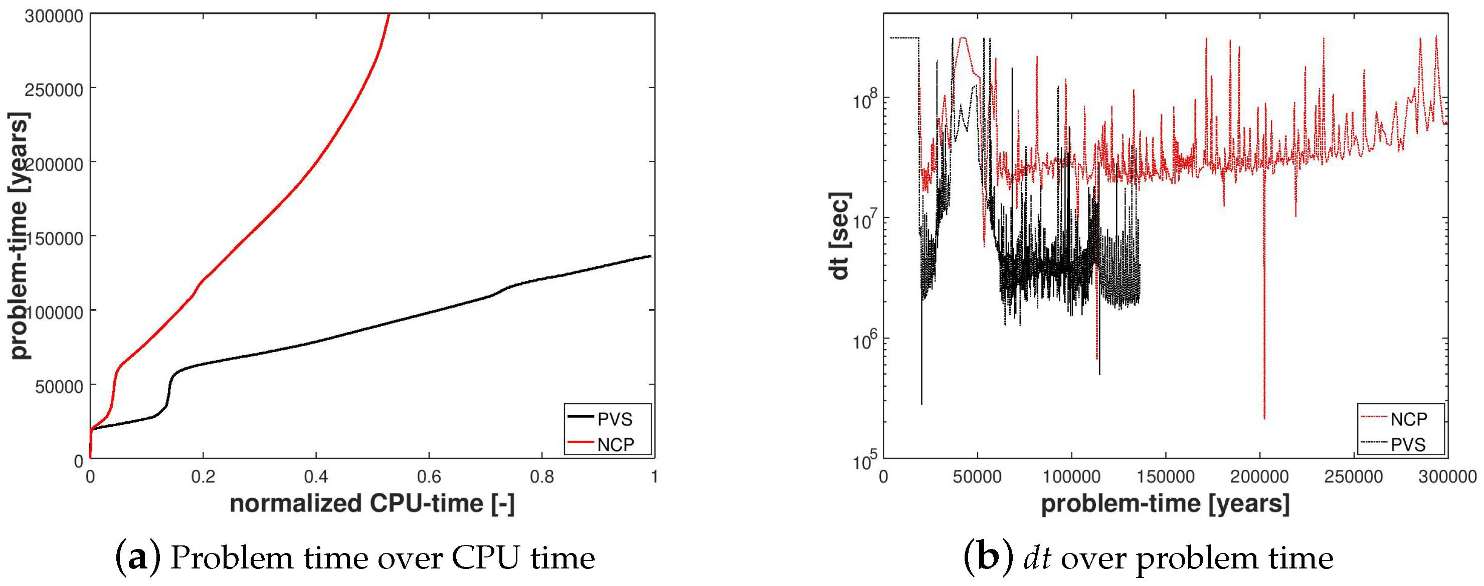
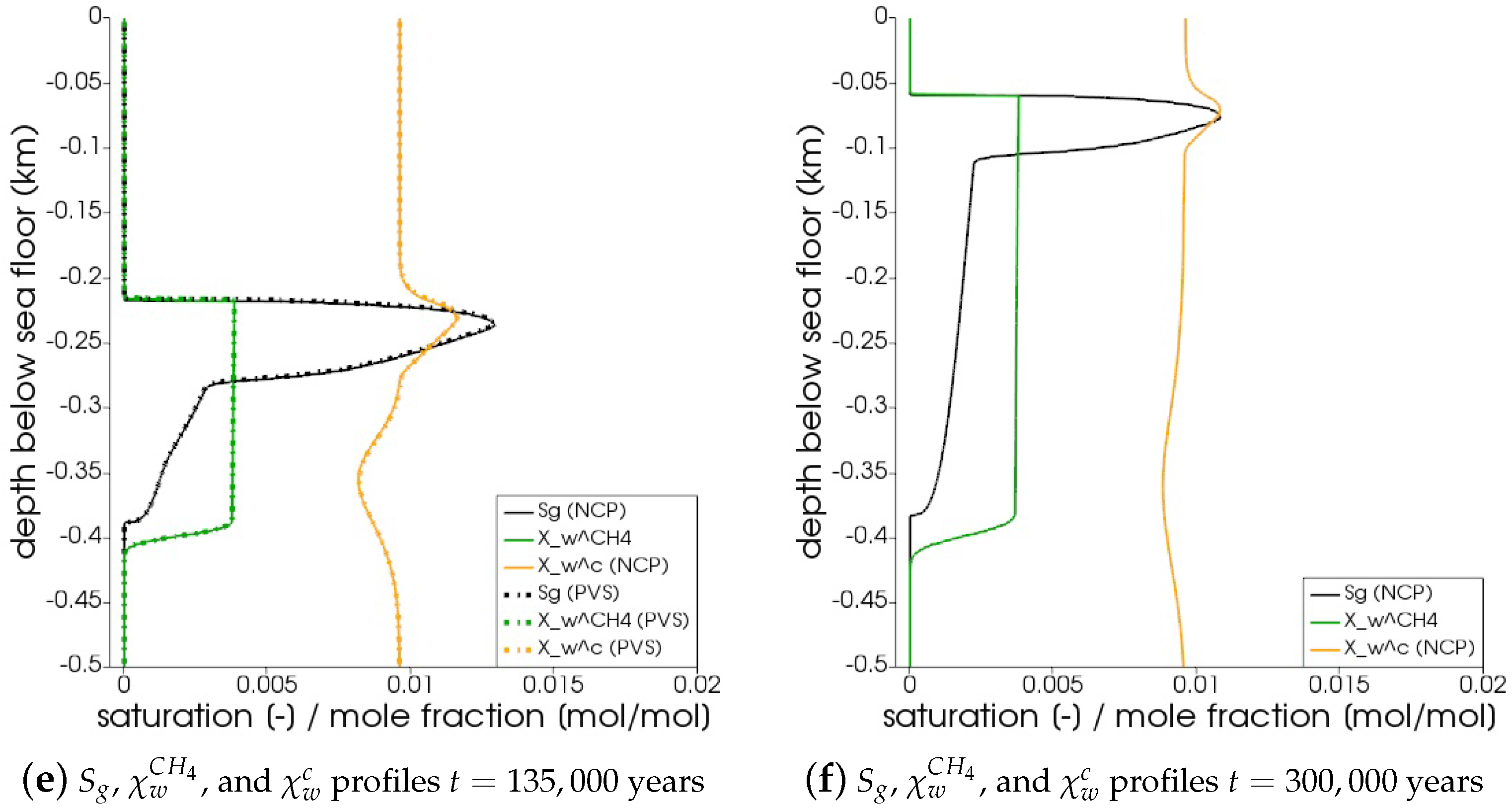
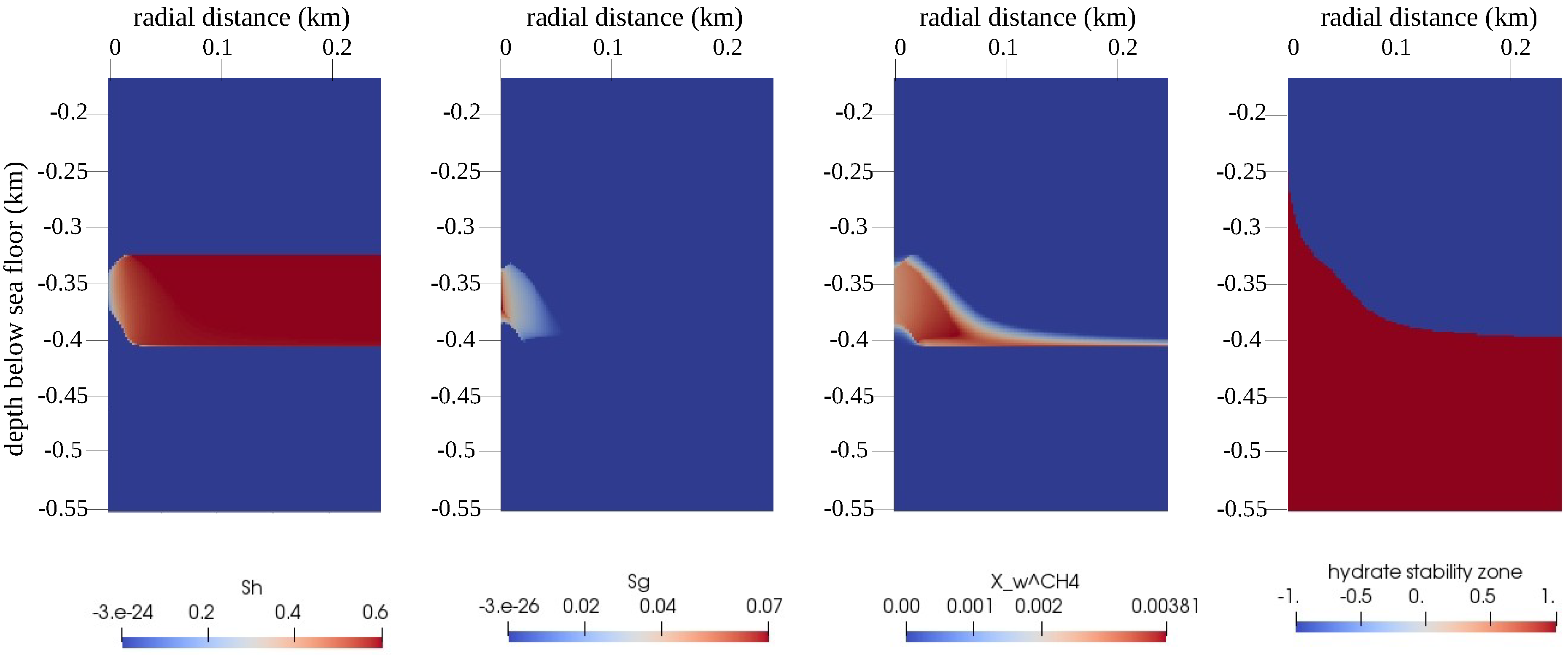
4.1.2. Numerical Simulation and Results

The computational domain was discretized uniformly into 1600 finite volumes along the Z-axis. The maximum time step size was chosen as d t m a x = 10 years. An adaptive time-stepping strategy was used where the time step size was controlled heuristically based on the number of Newton iterations per time integration step. If the number of Newton iterations was more than h , the time step size for the next time integration step was decreased by 25%, whereas if the number of Newton iterations was less than l , the time step size was increased by 10%. Between l and h Newton iterations, d t was not changed. The choice of l and h depends on the problem setting and, as a general rule, in our numerical scheme we considered l 4 and h = l + 4 . In this example, we chose l = 8 and h = 12 .
We performed the numerical simulations with our semi-smooth Newton (NCP) scheme, and for comparison, also with the more common primary variable switching (PVS) approach of [11]. We implemented this PVS scheme within the same software framework as our NCP approach (i.e., DUNE-PDElab, version 2.6.0; https://www.dune-project.org/modules/dune-pdelab/). For both schemes, we used the same discretization scheme (Section 3.1) and the same linear solver (SuperLU). For the Newton solver, we used the same convergence criteria, and for the adaptive time-stepping strategy, we used identical control parameters. Note that we implemented only a sequential version of the PVS scheme. Therefore, for those examples where we compared the solution of our NCP scheme with the PVS scheme, we performed all numerical simulations only in a sequential mode.
In Figure 4a, we can see that the PVS scheme needed ≈50% more CPU time to solve only until ≈45% of the problem time even though the PVS scheme needed less time per calculation due to fewer degrees of freedom compared to the NCP scheme.
In Figure 5, the snapshots of S h , S g , χ w C H 4 , and χ w c are plotted at three times: t 1 = 22,500 years, t 2 = 135,000 years, and t 3 = 300,000 years. Time t 1 corresponds to the instant when the gas phase first appears in the domain. We can see that both the PVS and the NCP schemes are in agreement about where the gas phase appears and in what saturation. Time t 2 corresponds to the time up to which the PVS scheme could solve in 240 CPU-hours (at which point the simulation was aborted due to the large run time). The results of the PVS and the NCP schemes match very well, and serve as a good validation for our numerical implementation. Time t 3 corresponds to the end-time for this problem. Only the solution of the NCP scheme is plotted for this time step. The base of the GHSZ shifts upwards by 300 m due to sedimentation over a period of 300,000 years. The results show that as the GHSZ risis towards the sea floor, the hydrate layer dissociates, generating methane below the base of the GHSZ. Through a combination of dissolution, diffusion, and buoyancy effects, methane transports into the GHSZ where the gas hydrate layer re-forms. The hydrate layer follows the base of the GHSZ, but shrinks along the way as more and more gas dissolves and diffuses away. In Figure 6, this process of hydrate dissociation → gas migration → hydrate reformation is shown in greater detail by zooming in on the time axis between 60,000 years t 120,000 years. These processes are quite complex and nonlinear. As the gas hydrate dissociates from the bottom, the free gas rises upwards with a decreasing speed due to a decreasing permeability in the hydrate phase. When the gas phase crosses the region with maximum S h , the speed of gas migration starts to increase until it escapes the hydrate layer on the other side, where a new hydrate layer starts to form, as shown in Figure 6c. This new hydrate layer continues to grow using the free gas supplied by the dissociation of the old hydrate layer, as shown in Figure 6c–e.
In Figure 4b, the evolution of d t is plotted over the problem time for both schemes. We can see that at t = 22 , 500 years, when the gas phase first appears, d t breaks down for both schemes. However, the reduction of d t for NCP scheme was not as severe as that for the PVS scheme. The time step size gradually recovers as the gas slowly migrates upwards through the hydrate layer, but breaks down again around t = 60 , 000 years, when the free gas crosses the region with peak S h .

4.2. Example 2: Gas Production through Depressurization

In this example, we simulated a gas production scenario where the gas hydrate reservoir was destabilized through depressurization. We considered a single-well configuration, and based the model parameters, material properties, and initial conditions within the reservoir on the geological setting of the Black Sea. The objective of this example was to demonstrate the robustness of our scheme in handling complex phase transitions even in those settings where the reaction rates are large, the hydrate phase distributions are highly heterogeneous, and the permeability typically varies over two-to-four orders of magnitude. Such settings are commonly found in natural gas hydrate systems which occur in turbidite formations containing thin hydrate layers sandwiched between thin layers of silty to clayey sediments.

4.2.1. Problem Setting

We considered a 2 D axisymmetric domain, Ω , having dimensions 1000 m × 1000 m, as shown in Figure 7. The sea floor, Ω s f , was prescribed at z = 0 m. The depressurization well, Ω w e l l , was located at r = 0 m, 0 m z 400 m. The bottom water temperature at the sea floor was T s f = 4 C, and the hydrostatic pressure at the sea floor was P s f = 15 MPa. We assumed that the absolute intrinsic permeability and the total porosity of the primary soil skeleton were K = 10 13 m 2 and ϕ = 0.3 , respectively. At t = 0 , we assumed that the domain was fully saturated with saline water, and there was no free gas phase in the domain. Additionally, the aqueous phase contained no dissolved methane. For the aqueous phase pressure, we considered a hydrostatic pressure gradient, and for the temperature, we prescribed a regional geothermal gradient along the depth, d z T G = 35 C/km. The bGHSZ was located at z = 400 m. We considered that an 80-m-thick gas hydrate layer, Ω H , existed right above the bGHSZ. To show the robustness of our scheme with respect to complex phase transitions, we prescribed a random distribution of the hydrate phase within this layer, s.t. the hydrate saturation ranged from 0.0 to 0.6 , and the corresponding absolute permeability ranged from 10 13 m 2 to 1.6 × 10 15 m 2 . For t > 0 , a pressure of P w Ω w e l l = 8 MPa was prescribed at the production well to simulate gas production through depressurization. At the sea floor, the temperature, pressure, and salinity conditions remained constant and equal to the initial values. At the bottom boundary, Ω B , the regional geothermal gradient was maintained. The initial and boundary conditions are listed in Table 3, and the material properties and model parameters are listed in Table 2.

4.2.2. Numerical Simulation and Results

The computational domain was discretized into a total of 20,276 quadrilateral elements. The gas production process was simulated until t e n d = 360 days. The maximum time step size was chosen as d t m a x = 36,000 s, and the time step size d t was controlled adaptively using the heuristic strategy discussed in Section 4.1.2 with l = 4 and h = 8 . The simulation was run in parallel on four processing units and required a total of 20 CPU-hours. We identified a domain of interest, Ω I , for the gas production process as: 0 m r 250 m, 150 m z 550 m. Outside this domain, pressure, temperature, and saturation profiles did not change much. However, the large size of the domain is necessary to ensure that effects of depressurization do not reach Ω R , and the geothermal gradient is maintained at Ω B .
The main quantities of interest (QoIs) for gas production in gas hydrate reservoirs are S h , S g , χ w C H 4 , and the GHSZ. The snapshots of the QoIs within Ω I are plotted in Figure 8 for times t = 10 days, t = 90 days, and t = 360 days. We can see that over a period of one year, roughly 100 m of the reservoir was effectively depressurized, and the hydrate layer was fully dissociated within a zone of roughly 15 m around the production well. Due to the relatively high pore pressures, most of the methane was produced from the aqueous phase, and the saturation of the free gas phase remained well below 10%.
We compared the performance of the numerical scheme for this example with that of a reference gas production test case. The setting of the reference test case was the same as described in Section 4.2.1, except that the hydrate distribution in Ω H was homogeneous and had a uniform saturation of 0.6 . A snapshot of the QoIs in Ω H for the reference test case is plotted in Figure 9 at time step t = 360 days. By comparing the behavior of the numerical solution with the reference test case, we can ensure that the random hydrate distribution did not introduce any artificial numerical artifacts in the numerical solution. In Figure 10, we can also see that despite the random distribution of the hydrate phase and the large variations in the sediment permeability, the semi-smooth Newton scheme was able to handle the phase transitions quite robustly without significant loss in performance, as indicated by the evolution of the time-step sizes.

5. Conclusions

In this article, we presented a mathematical model for non-isothermal multi-phase multi-component reactive transport processes in methane hydrate reservoirs. The methane hydrate phase transitions were modeled as a non-equilibrium based kinetic process, and the phase transitions within the C H 4 H 2 O system were modeled as a VLE process. The inequality conditions resulting from the VLE assumption were cast as Kharush–Kuhn–Tucker (KKT) equality conditions which were implemented within a semi-smooth Newton scheme using an active-set strategy. Note that in the context of gas hydrate models, a similar nonlinear complementary constraints approach was also used by [55] to develop a semi-smooth Newton strategy for solving a Stefan-type problem involving equilibrium-based hydrate phase transition.
In many widely used multi-phase multi-component gas hydrate reservoir simulators, PVS is the method of choice for handling phase transitions and the vanishing gas phase. In general, the PVS method has the advantage that the numerical model has fewer degrees of freedom, and therefore can perform numerical calculations faster. However, in the case of gas hydrate models, this advantage is most often lost because the phase transitions occur at different rates, and are highly coupled and extremely sensitive to the changes in the local thermodynamic state, which leads to rapidly switching phase states. The PVS scheme often shows poor convergence and requires much smaller time steps. We demonstrated this in Example 1 (Section 4.1), where we simulated gas migration through the GHSZ in the highly dynamic geological setting of the Black Sea over paleo time-scales. Note in Table 2 that, for Example 1, we greatly simplified the problem setting by neglecting the functional dependence of the material properties (e.g., densities, viscosities, heat capacities, and thermal conductivities) on local temperature, pressure, and salinity conditions, thereby reducing the nonlinearities, and we considered only a 1 D setting with homogeneous phase distributions across the domain. Despite these simplifications, the PVS scheme performed much more poorly compared to our semi-smooth Newton scheme. In Example 2 (Section 4.2), we considered another very important application of methane hydrate models, viz., gas production through depressurization. We considered a random distribution of the hydrate phase (and consequently, a random permeability field and capillary pressures ranging over multiple orders of magnitude). We also included strongly nonlinear functional dependencies of the material properties on the local thermodynamic state (see Table 2). Through this example we demonstrated that our semi-smooth Newton scheme can robustly handle even very complex field-scale problems.

Author Contributions

Conceptualization, S.G., B.W., and M.H.; methodology, S.G. and B.W.; software, S.G.; formal analysis, S.G.; writing—original draft preparation, S.G.; writing—review and editing, S.G.; visualization, S.G.; funding acquisition, S.G., M.H., B.W. All authors have read and agreed to the published version of the manuscript.

Funding

This research was funded by the Cluster of Excellence “The Future Ocean” and the SUGAR project. The Future Ocean is funded within the framework of the Excellence Initiative by the Deutsche Forschungsgemeinschaft (DFG) on behalf of the German federal and state governments. SUGAR was jointly funded by the German Ministry of Economy and Energy (BMWi) and the German Ministry of Education and Research (BMBF) through grant no. 03G0856A. We also acknowledge the support of DFG through project no.WO 671/11-1.

Conflicts of Interest

The authors declare no conflicts of interest.

References

  1. Suess, E. Marine cold seeps. In Handbook of Hydrocarbon and Lipid Microbiology; Timmis, K.N., Ed.; Springer-Verlag: Berlin/Heidelberg, Germany, 2010; Volume 1, pp. 187–203. [Google Scholar] [CrossRef]
  2. Liu, J.; Haeckel, M.; Rutqvist, J.; Wang, S.; Yan, W. The Mechanism of Methane Gas Migration through the Gas Hydrate Stability Zone: Insights From Numerical Simulations. J. Geophys. Res. Solid Earth 2019, 124, 4399–4427. [Google Scholar] [CrossRef] [Green Version]
  3. Piñero, E.; Marquardt, M.; Hensen, C.; Haeckel, M.; Wallmann, K. Estimation of the global inventory of methane hydrates in marine sediments using transfer functions. Biogeosciences 2013, 10, 959–975. [Google Scholar] [CrossRef] [Green Version]
  4. Burwicz, E.; Rüpke, L.; Wallmann, K. Estimation of the global amount of submarine gas hydrates formed via microbial methane formation based on numerical reaction-transport modeling and a novel parameterization of Holocene sedimentation. Geochim. Cosmochim. Acta 2011, 75, 4562–4576. [Google Scholar] [CrossRef] [Green Version]
  5. Archer, D.; Buffett, B.; Brovkin, V. Ocean methane hydrates as a slow tipping point in the global carbon cycle. Proc. Natl. Acad. Sci. USA 2009, 106, 20596–20601. [Google Scholar] [CrossRef] [PubMed] [Green Version]
  6. Wang, F.; Zhao, B.; Li, G. Prevention of Potential Hazards Associated with Marine Gas Hydrate Exploitation: A Review. Energies 2018, 11, 2384. [Google Scholar] [CrossRef] [Green Version]
  7. Ruppel, C.D.; Kessler, J.D. The interaction of climate change and methane hydrates. Rev. Geophys. 2017, 55, 126–168. [Google Scholar] [CrossRef]
  8. Class, H.; Helmig, R.; Niessner, J.; Ölmann, U. Multiphase processes in porous media. Lect. Notes Appl. Comput. Mech. 2006, 2006, 45–82. [Google Scholar] [CrossRef]
  9. Marchand, E.; Müller, T.; Knabner, P. Fully coupled generalized hybrid-mixed finite element approximation of two-phase two-component flow in porous media. Part I: Formulation and properties of the mathematical model. Comput. Geosci. 2013, 17, 431–442. [Google Scholar] [CrossRef]
  10. Wu, Y.S.; Forsyth, P.A. On the selection of primary variables in numerical formulation for modeling multiphase flow in porous media. J. Contam. Hydrol. 2001, 48, 277–304. [Google Scholar] [CrossRef]
  11. Class, H.; Helmig, R.; Bastian, P. Numerical simulation of non-isothermal multiphase multicomponent processes in porous media. 1. An efficient solution technique. Adv. Water Resour. 2002, 25, 533–550. [Google Scholar] [CrossRef]
  12. Panfilov, M.; Panfilova, I. Method of negative saturations for flow with variable number of phases in porous media: Extension to three-phase multi-component case. Comput. Geosci. 2014, 18, 385–399. [Google Scholar] [CrossRef]
  13. Neumann, R.; Bastian, P.; Ippisch, O. Modeling and simulation of two-phase two-component flow with disappearing nonwetting phase. Comput. Geosci. 2013, 17, 139–149. [Google Scholar] [CrossRef] [Green Version]
  14. Huang, Y.; Kolditz, O.; Shao, H. Extending the persistent primary variable algorithm to simulate non-isothermal two-phase two-component flow with phase change phenomena. Geotherm. Energy 2015, 3. [Google Scholar] [CrossRef] [Green Version]
  15. Lauser, A.; Hager, C.; Helmig, R.; Wohlmuth, B. A new approach for phase transitions in miscible multi-phase flow in porous media. Adv. Water Resour. 2011, 34, 957–966. [Google Scholar] [CrossRef]
  16. Kräutle, S. The semismooth Newton method for multicomponent reactive transport with minerals. Adv. Water Resour. 2011, 34, 137–151. [Google Scholar] [CrossRef]
  17. Ben-Gharbia, I.; Jaffré, J. Gas phase appearance and disappearance as a problem with complementarity constraints. Math. Comput. Simul. 2014, 99, 28–36. [Google Scholar] [CrossRef] [Green Version]
  18. Bui, Q.M.; Elman, H.C. Semi-smooth Newton methods for nonlinear complementarity formulation of compositional two-phase flow in porous media. arXiv 2018, arXiv:1805.05801. [Google Scholar] [CrossRef] [Green Version]
  19. Moridis, G.; Kowalsky, M.B.; Pruess, K. TOUGH + Hydrate v1.0 User’s Manual: A Code for the Simulation of System Behavior in Hydrate-Bearing Geologic Media; LBNL: Berkeley, CA, USA, 2008. [Google Scholar] [CrossRef] [Green Version]
  20. Janicki, G.; Schlüter, S.; Hennig, T.; Lyko, H.; Deerberg, G. Simulation of Methane Recovery from Gas Hydrates Combined with Storing Carbon Dioxide as Hydrates. J. Geol. Res. 2011, 2011. [Google Scholar] [CrossRef] [Green Version]
  21. Janicki, G.; Schlöter, S.; Hennig, T.; Deerberg, G. Simulation of subsea gas hydrate exploitation. Energy Procedia 2014, 59, 82–89. [Google Scholar] [CrossRef]
  22. White, M.D.; Appriou, D.; Bacon, D.H.; Fang, Y.; Freedman, V.; Rockhold, M.L.; Ruprecht, C.; Tartakovsky, G.; White, S.K.; Zhang, F. STOMP Online User Guide; Pacific Northwest National Laboratory: Richland, WA, USA, 2015. [Google Scholar]
  23. Moridis, G.J.; Kowalsky, M.B.; Pruess, K. HYDrateResSim User’S Manual: A Numerical Simulator for Modeling the Behaviour of Hydrates in Geologic Media; Earth Sciences Division, Lawrence Berkeley National Laboratory: Berkeley, CA, USA, 2005. [Google Scholar]
  24. Liu, X.; Flemings, P.B. Dynamic multiphase flow model of hydrate formation in marine sediments. J. Geophys. Res. Solid Earth 2007, 112. [Google Scholar] [CrossRef] [Green Version]
  25. Gupta, S.; Helmig, R.; Wohlmuth, B. Non-isothermal, multi-phase, multi-component flows through deformable methane hydrate reservoirs. Comput. Geosci. 2015, 19, 1063–1088. [Google Scholar] [CrossRef] [Green Version]
  26. Fuente, M.D.L.; Vaunat, J.; Marín-Moreno, H. Thermo-Hydro-Mechanical Coupled Modeling of Methane Hydrate-Bearing Sediments: Formulation and Application. Energies 2019, 12, 2178. [Google Scholar] [CrossRef] [Green Version]
  27. Sánchez, M.; Santamarina, C.; Teymouri, M.; Gai, X. Coupled Numerical Modeling of Gas Hydrate-Bearing Sediments: From Laboratory to Field-Scale Analyses. J. Geophys. Res. Solid Earth 2018, 123, 10326–10348. [Google Scholar] [CrossRef] [Green Version]
  28. Helmig, R. Multiphase Flow and Transport Processes in the Subsurface. A Contribution to the Modeling of Hydrosystems; Springer: Berlin/Heidelberg, Germany, 1997; p. 367. [Google Scholar]
  29. Facchinei, F.; Pang, J.S. Finite-Dimensional Variational Inequalities and Complementarity Problems, Volume II; Springer: New York, NY, USA, 2013; Volume 53, pp. 1689–1699. [Google Scholar] [CrossRef]
  30. Trémolières, R.; Lions, J.; Glowinski, R. Numerical Analysis of Variational Inequalities; Studies in Mathematics and its Applications; Elsevier Science: Amsterdam, The Netherlands, 2011. [Google Scholar]
  31. Hager, C.; Wohlmuth, B. Semismooth Newton methods for variational problems with inequality constraints. GAMM Mitt. 2010, 33, 8–24. [Google Scholar] [CrossRef]
  32. Hintermüller, M.; Ito, K.; Kunisch, K. The Primal-Dual Active Set Strategy As a Semismooth Newton Method. SIAM J. Optim. 2002, 13, 865–888. [Google Scholar] [CrossRef] [Green Version]
  33. Hüeber, S.; Wohlmuth, B. A primal-dual active set strategy for non-linear multibody contact problems. Comput. Methods Appl. Mech. Eng. 2005, 194, 3147–3166. [Google Scholar] [CrossRef]
  34. Hassanizadeh, M.; Gray, W.G. General conservation equations for multi-phase systems: 1. Averaging procedure. Adv. Water Resour. 1979, 2, 131–144. [Google Scholar] [CrossRef]
  35. Hassanizadeh, M.; Gray, W.G. General conservation equations for multi-phase systems: 2. Mass, momenta, energy, and entropy equations. Adv. Water Resour. 1979, 2, 191–203. [Google Scholar] [CrossRef]
  36. Hassanizadeh, M.; Gray, W.G. General conservation equations for multi-phase systems: 3. Constitutive theory for porous media flow. Adv. Water Resour. 1980, 3, 25–40. [Google Scholar] [CrossRef]
  37. Kuhn, H.W.; Tucker, A.W. Nonlinear Programming. In Proceedings of the Second Berkeley Symposium on Mathematical Statistics and Probability, Berkeley, CA, USA, 31 July–12 August 1950; University of California Press: Berkeley, CA, USA, 1951; pp. 481–492. [Google Scholar]
  38. Kim, H.C.; Bishnoi, P.R.; Heidemann, R.A.; Rizvi, S.S.H. Kinetics of methane hydrate decomposition. Chem. Eng. Sci. 1987, 42, 1645–1653. [Google Scholar] [CrossRef]
  39. Kamath, V. Study of Heat Transfer Characteristics During Dissociation of Gas Hydrates in Porous Media. Ph.D. Thesis, University of Pittsburgh, Pittsburgh, PA, USA, 1984. [Google Scholar]
  40. Brooks, R.H.; Corey, A.T. Hydraulic Properties of Porous Media; Colorado State University Hydrology Papers, Colorado State University: Fort Collins, CO, USA, 1964. [Google Scholar]
  41. Gupta, S. Non-Isothermal, Multi-Phase, Multi-Component Flows through Deformable Methane Hydrate Reservoirs. Ph.D. Thesis, Technical University of Munich: Munich, Germany, 2016. [Google Scholar]
  42. Kossel, E.; Deusner, C.; Bigalke, N.; Haeckel, M. The Dependence of Water Permeability in Quartz Sand on Gas Hydrate Saturation in the Pore Space. J. Geophys. Res. Solid Earth 2018, 123, 1235–1251. [Google Scholar] [CrossRef] [Green Version]
  43. Chen, B.; Chen, X.; Kanzow, C. A penalized Fischer-Burmeister NCP-function. Math. Program. 2000, 88, 211–216. [Google Scholar] [CrossRef]
  44. Fischer, A. On the local superlinear convergence of a Newton-type method for LCP under weak conditions. Optim. Methods Softw. 1995, 6, 83–107. [Google Scholar] [CrossRef]
  45. Fischer, A. A Newton-type method for positive-semidefinite linear complementarity problems. J. Optim. Theory Appl. 1995, 86, 585–608. [Google Scholar] [CrossRef]
  46. Fischer, A. A special newton-type optimization method. Optimization 1992, 24, 269–284. [Google Scholar] [CrossRef]
  47. Bastian, P.; Heimann, F.; Marnach, S. Generic implementation of finite element methods in the Distributed and Unified Numerics Environment (DUNE). Kybernetika 2010, 46, 294–315. [Google Scholar]
  48. Demmel, J.W.; Eisenstat, S.C.; Gilbert, J.R.; Li, X.S.; Liu, J.W.H. A supernodal approach to sparse partial pivoting. SIAM J. Matrix Anal. Appl. 1999, 20, 720–755. [Google Scholar] [CrossRef]
  49. Winguth, C.; Wong, H.; Panin, N.; Dinu, C.; Georgescu, P.; Ungureanu, G.; Krugliakov, V.; Podshuveit, V. Upper Quaternary water level history and sedimentation in the northwestern Black Sea. Mar. Geol. 2000, 167, 127–146. [Google Scholar] [CrossRef]
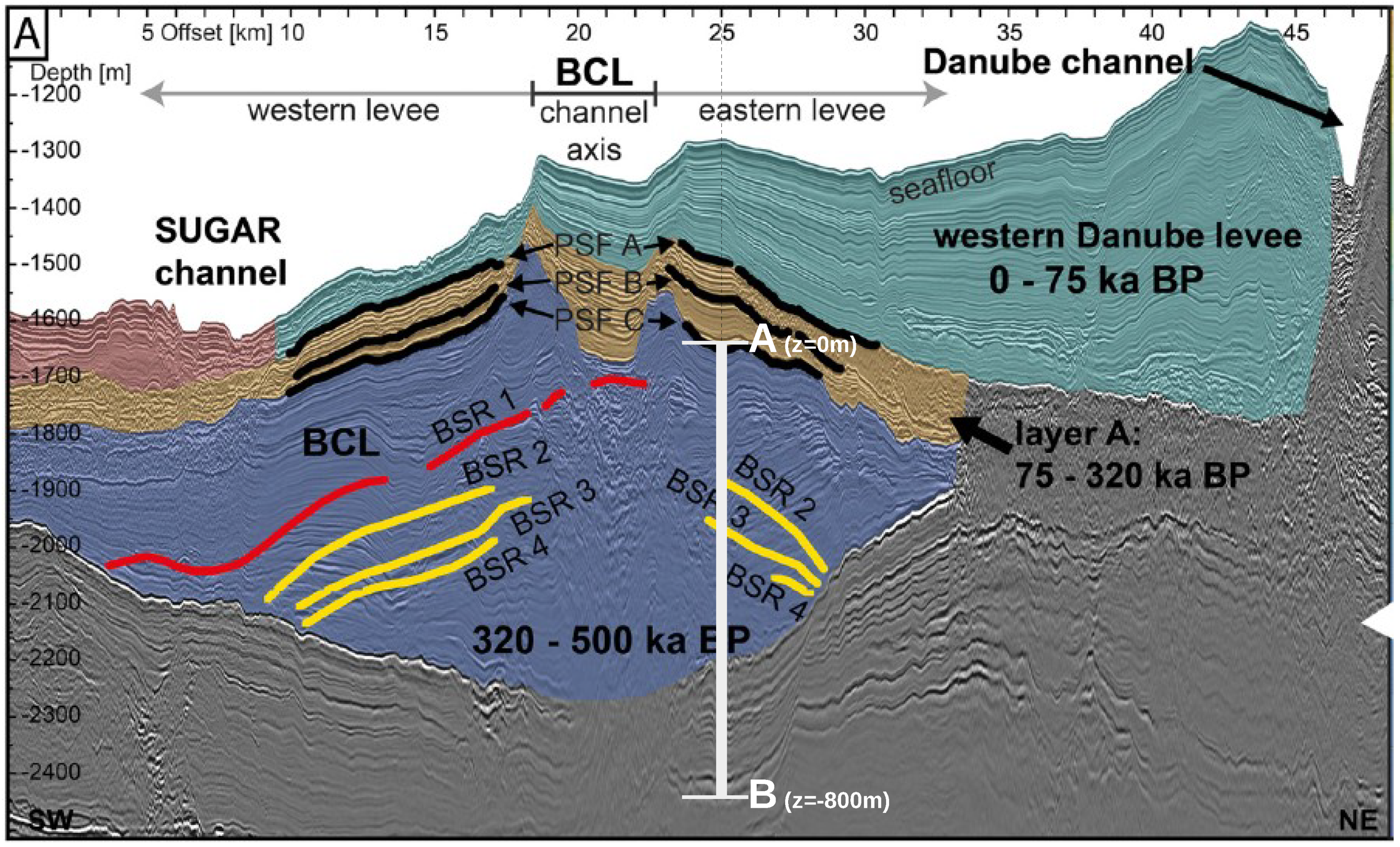
  50. Zander, T.; Haeckel, M.; Berndt, C.; Chi, W.C.; Klaucke, I.; Bialas, J.; Klaeschen, D.; Koch, S.; Atgın, O. On the origin of multiple BSRs in the Danube deep-sea fan, Black Sea. Earth Planet. Sci. Lett. 2017, 462, 15–25. [Google Scholar] [CrossRef] [Green Version]
  51. Degens, E.T.; Ross, D.A. The Black Sea: Geology, chemistry, biology. AAPG Mem. 1974. [Google Scholar] [CrossRef]
  52. Peng, D.Y.; Robinson, D.B. A New Two-Constant Equation of State. Ind. Eng. Chem. Fundam. 1976, 15, 59–64. [Google Scholar] [CrossRef]
  53. Kossel, E.; Bigalke, N.; Pinero, E.; Haeckel, M. The SUGAR Toolbox—A Library of Numerical Algorithms and Data for Modelling of Gas Hydrate Systems and Marine Environments; Technical Report Report Nr. 8:160; GEOMAR: Kiel, Germany, 2013. [Google Scholar]
  54. Gupta, S.; Deusner, C.; Haeckel, M.; Helmig, R.; Wohlmuth, B. Testing a thermo-chemo-hydro-geomechanical model for gas hydrate-bearing sediments using triaxial compression laboratory experiments. Geochem. Geophys. Geosyst. 2017, 18, 3419–3437. [Google Scholar] [CrossRef] [Green Version]
  55. Gibson, N.L.; Patricia Medina, F.; Peszynska, M.; Showalter, R.E. Evolution of phase transitions in methane hydrate. J. Math. Anal. Appl. 2014, 409, 816–833. [Google Scholar] [CrossRef]
Figure 1. Representation of the phases and components in a representative elementary volume (REV). For any pore-filling phase β = g , w , h , phase saturation is defined as S β : = V β V p . Total and apparent porosites are defined as ϕ : = V p V t , and ϕ e f f : = V p V h V t = 1 S h ϕ , respectively.
Energies 13 00503 g001
Figure 2. Regional seismic profile across the western part of the Danube paleo delta in SW to NE direction, depicting the geological setting for Example 1 (Section 4.1). 2D RMCS line 09. Interpretation of the seismic data according to [50]. BCL: buried channel-levee.
Energies 13 00503 g002
Figure 3. Problem setting for Example 1 (Section 4.1). (a) The initial state of the system and identifies the corresponding gas hydrate stability zone (GHSZ). (b) The state of the system at t = t n > 0 , illustrating how the GHSZ shifts as a result of sedimentation over time.
Energies 13 00503 g003
Figure 4. Numerical results for Example 1 (Section 4.1). The figure compares the NCP and the primary variable switching (PVS) schemes in terms of the cumulative CPU time required to solve the problem and the evolution of the time-step size during the simulation.
Energies 13 00503 g004
Figure 5. Numerical results for Example 1 (Section 4.1). The figure shows snapshots of S h , S g , χ w C H 4 , and χ w c at t = 22,500 years, that is, the time when the gas phase first appears; t = 135,000 years, that is, the time up to which the PVS scheme solved in 240 CPU-hours; and t = t e n d = 300,000 years. For t = 22,500 years and t = 135,000 years, the solutions of both NCP and PVS schemes is plotted for comparison.
Energies 13 00503 g005aEnergies 13 00503 g005b
Figure 6. Numerical results for Example 1 (Section 4.1). Figure shows the process of hydrate dissociation → gas migration → hydrate reformation as a result of rising GHSZ between 60,000 years t 120,000 years. The new gas hydrate layer grows using the methane gas supplied by the dissociating gas hydrate layer below.
Energies 13 00503 g006aEnergies 13 00503 g006bEnergies 13 00503 g006c
Figure 7. Problem setting for Example 2 (Section 4.2). Figure (a) highlights the essential features of the problem setting like the locations of the sea floor, the production well, the initial base of the GHSZ, and the initial hydrate distribution within the hydrate layer, and marks our domain of interest within the computational domain. Figure (b) identifies the relevant regions of the computational domain. Ω denotes the computational domain, Ω H Ω denotes the hydrate layer, Ω I Ω denotes the domain of interest, and Ω H Ω I . Ω w e l l denotes the production well boundary, while Ω L denotes the left boundary excluding the production well. Ω s f denotes the top boundary corresponding to the sea floor. Ω R and Ω B denote the right and the bottom boundaries, respectively.
Energies 13 00503 g007
Figure 8. Numerical results for Example 2 (Section 4.2). The figure shows snapshots of the quantities of interest (QoIs) (from left to right: S h , S g , χ w C H 4 , and the GHSZ) within the domain of interest Ω I at different times. Note that for GHSZ, a value of 1 indicates an unstable zone, and 1 indicates a stable zone.
Energies 13 00503 g008
Figure 9. Numerical results for the reference test case of Example 2 (Section 4.2). The figure shows snapshots of the QoIs (from left to right: S h , S g , χ w C H 4 , and the GHSZ) within the domain of interest Ω I at t = t e n d = 360 days. Note that for the GHSZ, 1 indicates an unstable zone, and 1 indicates a stable zone.
Energies 13 00503 g009
Figure 10. Numerical result for Example 2 (Section 4.2). A comparison of the time-step size evolution for a random hydrate phase distribution and a homogeneous hydrate phase distribution.
Energies 13 00503 g010
Table 1. Initial and bounday conditions for Example 1 (Section 4.1).
Initial Conditions
at t = 0 , and 0 m z 800 m P w = P s f + ρ w g z s f z
where z s f = 0 m is the sea floor,
and P s f = 15 MPa is the water pressure at the sea floor.
T= T s f + d z T G z s f z
where T s f = 4 C is the bottom water temperature,
and d z T G = 35 C / km denotes the regional geothermal temperature gradient.
S g =0
χ w C H 4 =0
χ g H 2 O = χ g , s a t H 2 O P g t = 0 , T t = 0
χ w c = 5.5 mmol / mol
at t = 0 ,
      if,     320 m z 400 m, S h = 0.3 400 + z 400 320 z + 320 400 320
else if,     z > 320 m or z < 400 m S h =0
Boundary Conditions
t > 0 , and  z = 0 m P w = P s f + ρ s g v s , z t n + Δ t
T= T s f + d z T G v s , z t n + Δ t
S g =0
χ w c = χ w c t = 0
t > 0 , and  z = 800 m z P w =0
z T = d z T G
v g , z =0
z χ w c =0
Table 2. Material properties and model parameters for Examples 1 and 2.
Property 1 , 2 Example 1Example 2
Water
density ρ w kg/m 3 1030.21 1027 + 0.45 P w MPa 0.15 T C 10 + 0.3521 × 10 3 χ w c 0.0096
dynamic viscosity μ w Pa.s 0.00136 0.001792 exp 0 1.94 4.80 273.15 T + 6.75 273.15 T 2
thermal conductivity k w t h W/m/K 0.59 0.57153 1 + 0.003 T C 1.025 × 10 5 T C 2 + 6.53 × 10 10 P w 0.0797 χ w c
specific heat capacity C p w J/kg/K3945
saturation vapor pressure P s a t H 2 O Pa P c exp 1 T r c 1 ( 1 T r ) + c 2 ( 1 T r ) 1.5 + c 3 ( 1 T r ) 3 + c 4 ( 1 T r ) 3.5 + c 5 ( 1 T r ) 4 + c 6 ( 1 T r ) 7.5
where P c = 22.064 MPa, T c = 647.096 K, T r = T / T c , and  c 1 = 7.85951783 , c 2 = 1.84408259 , c 3 = 11.7866497 , c 4 = 22.6807411 , c 5 = 15.9618719 , c 6 = 1.80122502 .
diffusion coefficient D g H 2 O m 2 /s 0.638 × 10 6 2.26 × 10 9 T + 0.002554 P g
Methane
density ρ g kg/m 3 0.002756 P g T P g z C H 4 R C H 4 T    where R C H 4 = 8314.5 16.04 , and  z C H 4 is estimated using Peng Robinson EoS [52].
dynamic viscosity μ g Pa.s 1.4055 × 10 5 μ 0 273.15 + 162 T + 162 T 273.15 1.5
where μ 0 = 1.0707 × 10 5 4.8134 × 10 14 P g 4.1719 × 10 20 P g 2 + 7.3232 × 10 28 P g 3
thermal conductivity k g t h W/m/K 0.03121 a 0 + a 1 T + a 2 T 2 + a 3 T 3
where a 0 = 0.008863 , a 1 = 0.000242 , a 2 = 0.6997 × 10 6 , and  a 3 = 0.1225 × 10 8
specific heat capacity C p g J/kg/K 2168.65 1238 + 3.13 T + 7.905 × 10 4 T 2 6.858 × 10 7 T 3
solubility constant H w C H 4 Pa exp log ( P s a t H 2 O ) 11.0094 T r + 4.8362 ( 1 T r ) 0.355 T r + 12.5220 exp ( 1 T r ) T r 0.41
diffusion coefficient D w C H 4 m 2 /s 1.57 × 10 11 1.57 × 10 11 P w 1.0135 × 10 5 exp 0.003475 T
Hydrate
density ρ h kg/m 3 920
hydration number N h 5.90
thermal conductivity k h t h W/m/K 0.5
specific heat capacity C p h J/kg/K2327 1.937 T 3 1.5151 T 2 + 3.9554 T 342.7 × 10 3
Salt
diffusion coefficient D w c m 2 /s 10 9
Soil
density ρ s kg/m 3 2600
thermal conductivity k s t h W/m/K 3.0
specific heat capacity C p s J/kg/K1000
Hydrate Phase Change Kinetics
hydrate equilibrium pressure P e Pa exp 38.592 8533.8 T + 4.4824 χ w c
kinetic rate constant k r mol/m 2 /Pa/s 10 17 10 12
specific surface area A 0 m 2 /m 3 10 5
heat of reaction Q ˙ h W/m 3 g ˙ h M h 56599 16.744 T
Hydraulic Properties
absolute intrinsic permeability K 0 m 2 10 15 10 13
total porosity ϕ 0.5 0.3
Brooks–Corey parameters p 0 , λ Pa,− 5 × 10 4 , 1.2
sphericity parameterm1
residual saturations S w r , S g r −,−0,0
1 See [53] for references to P s a t H 2 O an H w C H 4 ; [20] for references to k w t h , C p w , μ 0 , g , ρ h , N h , k h t h , C p h , D w c , ρ s , k s t h , and C p s ; and [54] for references to μ w , D g H 2 O , μ g , D w C H 4 , k g t h , C p g , and Q ˙ h . 2 To evaluate the property values for Example 1, we considered a reference state of T = 9 C, P = 10 MPa , and χ w c = 5.5 mmmol/mol.
Table 3. Initial and bounday conditions for Example 2 (Section 4.2).
Initial Conditions
tag: Ω
at t = 0 ,
0 m r 1000 m and 0 m z 1000 m
P w = P s f + ρ w g z s f z
where z s f denotes the sea floor, z s f = 0 m,
and P s f denotes the water pressure at the sea floor, P s f = 15 MPa.
T= T s f + d z T G z s f z
where T s f = 4 C denotes the temperature at the sea floor,
and, d z T G = 35 C / km denotes the regional geothermal temperature gradient.
S g =0
χ w C H 4 =0
χ g H 2 O = χ g , s a t H 2 O P g t = 0 , T t = 0
χ w c = 5.5 mmol / mol
at t = 0 , and  0 m r 1000 m,
tag: Ω H :        320 m z 400 m S h =rand 0 , 0.6
tag: Ω Ω H :     z > 320 m or z < 400 m S h =0
Boundary Conditions
tag: Ω w e l l P w = 8 MPa
t > 0 ,     r = 0 and 0 m z 400 m T =0
v g =0
χ w c =0
tag: Ω s f P w = P s f
t > 0 ,     z = 0 and 0 m r 1000 mT= T s f
S g =0
χ w c = χ w c t = 0
tag: Ω R v w =0
t > 0 ,     r = 1000 m and 0 m z 1000 m T =0
v g =0
χ w c g =0
tag: Ω B v w =0
t > 0 ,     z = 1000 m and 0 m r 1000 m T = T G
v g =0
χ w c g =0
tag: Ω L v w =0
t > 0 ,     r = 0 m and 400 m > z 1000 m T =0
v g =0
χ w c g =0

