A Temperature-Risk and Energy-Saving Evaluation Model for Supporting Energy-Saving Measures for Data Center Server Rooms

Abstract
:1. Introduction
2. Verification Data Conditions
2.1. Verification Room
2.2. Verification Data
3. Construction of Prediction Model
3.1. Aim of Each Construction Model
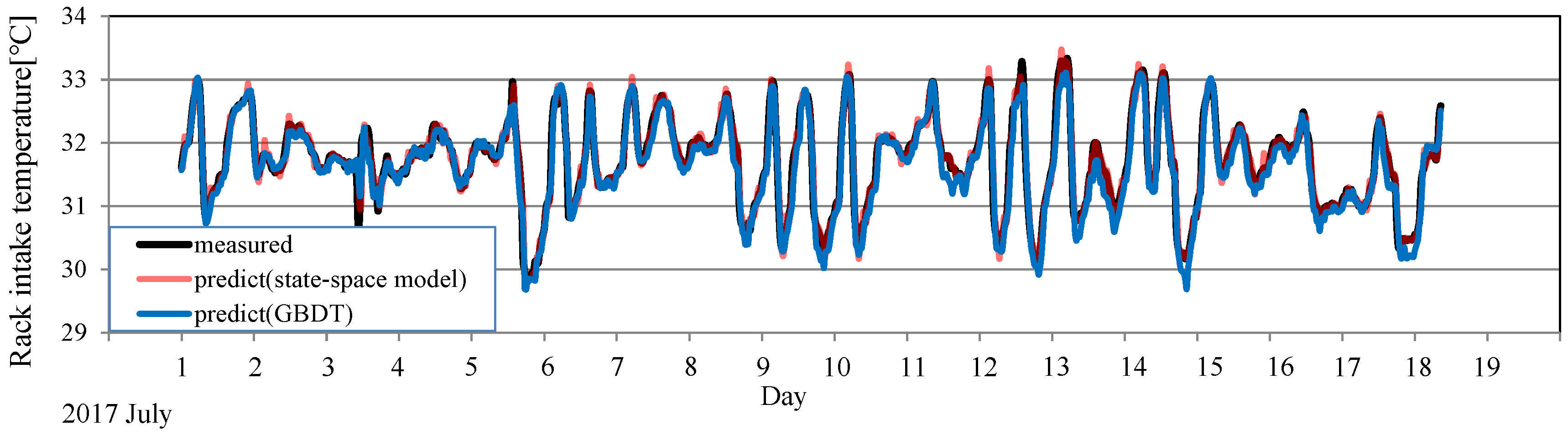
3.2. Outline of Prediction Model of Rack Intake Temperature
3.2.1. Construction of Model for Predicting Rack Intake Temperature
3.2.2. Methods Used by the Model for Predicting Rack Intake Temperature
3.2.3. Method for Evaluating the Model for Predicting Rack Intake Temperature
- Correlation coefficient (R): R expresses the explanatory power of the predicted value of the objective variable.
- Correct answer rate: The ratio of the number of predicted values within ±0.5 °C of the measured value to the total number of predicted values
- Root-mean-square error (RMSE): The accuracy of the three machine-learning methods is evaluated in terms of RMSE, which is a commonly used index for numerical prediction.
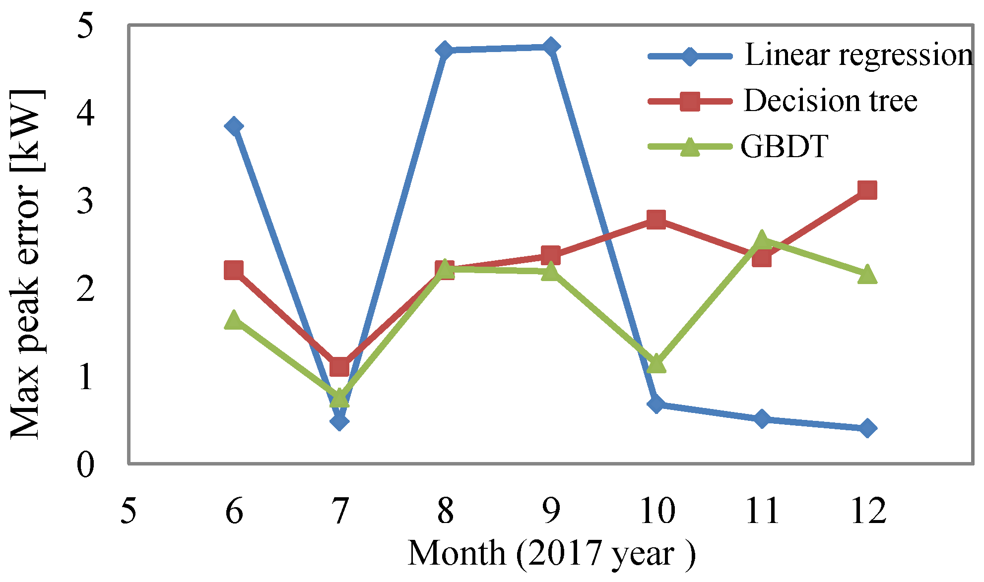
- Maximum peak error: As for predicting server-room temperature, maximum peak error is significant if the actual measured value and the predicted value deviate greatly. The error by which the actually measured value is larger than the predicted value is therefore defined as maximum peak error.
3.3. Outline of Baseline Model of CRAC
3.3.1. Construction of a Baseline Model for CRAC
3.3.2. Methods Used by Baseline Model
3.3.3. Method for Evaluating Baseline Model
- 1.
- Correlation coefficient (R): R expresses the explanatory power of the predicted value of the objective variable.
- 3.
- Root-mean-square error (RMSE): The accuracy of the three machine-learning methods is evaluated in terms of RMSE, which is a commonly used index for numerical prediction.
- 4.
- Maximum peak error: As for predicting server-room temperature, maximum peak error is significant if the actual measured value and the predicted value deviate greatly. The error by which the actually measured value is larger than the predicted value is therefore defined as maximum peak error.
- 5.
- Normalized Mean Bias Error (NMBE): NMBE is a normalization of the MBE index that is used to scale the results of MBE, making them comparable. This index is used by IPMVP.
4. Results
4.1. Evaluation of Accuracy of Temperature-Prediction Model
4.1.1. Primary Evaluation of Prediction Model and Narrowing Down of Prediction Methods
4.1.2. Secondary Evaluation of Prediction Model and Determination of Prediction Method
4.1.3. Detailed Evaluation of the Determined Prediction Model
- Effect of explanatory variables on accuracy
- 2.
- Effect of learning period on accuracy
4.1.4. Summary of Evaluation of Accuracy of Temperature Prediction Model
4.2. Evaluation of Accuracy of Baseline Model
4.2.1. Primary Evaluation of Baseline Model and Narrowing Down of Prediction Methods
4.2.2. Secondary Evaluation of Baseline Model and Determination of Prediction Method
4.2.3. Detailed Evaluation of Baseline Model
- 1.
- Effect of explanatory variables on prediction accuracy
- 2.
- Effect of learning period on accuracy
4.2.4. Summary of Evaluation of Accuracy of the Baseline Model
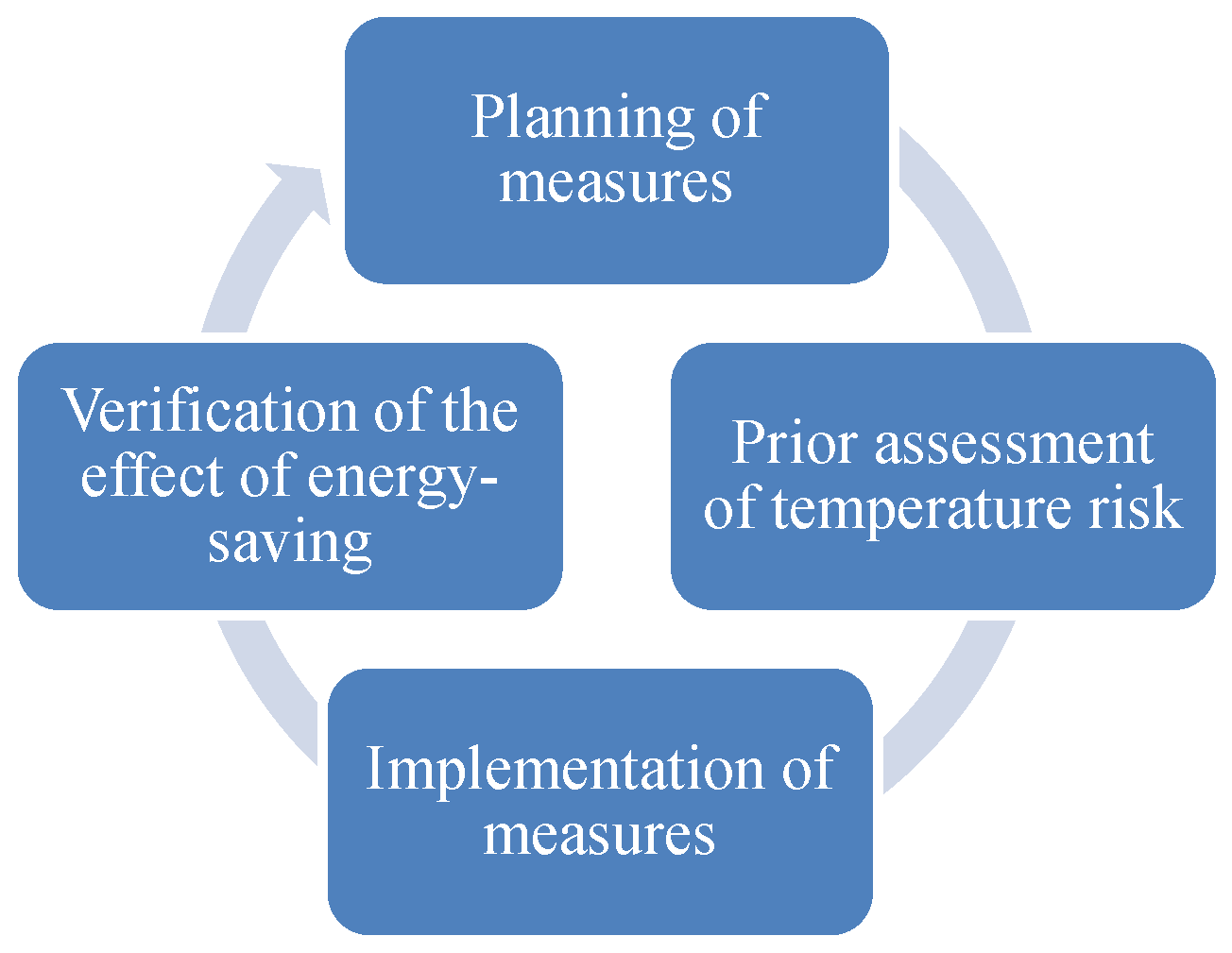
5. Verification of Effectiveness of the Proposed Model When Energy-Saving Measures Are Implemented
5.1. Overview of Effectiveness Verification
5.2. Evaluation of Temperature Risk by Using Rack Intake Temperature Prediction Model
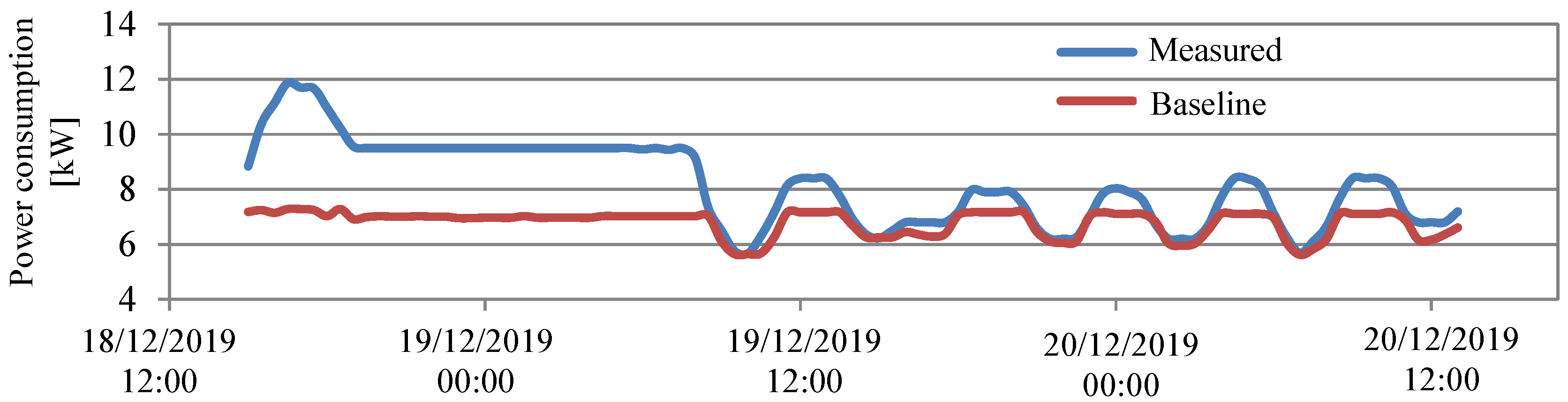
5.3. Visualization of Energy-Saving Effect by Using Baseline Model
5.4. Additional Verification of Baseline When the Setting of CRAC Return Temperature Is Changed
6. Concluding Remarks
- ■
- Prediction of rack intake temperature
- We defined an evaluation indices that we considered to be important of data center operation, and verified it with multiple machine learnng methods which has character of self-learning. I built a model which predicted using a state space model as a method high accuracy from the viewpoint of the evaluation indices.
- It was clarified that the return temperature of CRAC is an important among the explanatory variables on this model.
- ■
- Calculation of the CRAC baseline
- We selected a machine learning method with XAI that we thought was important in this problem.
- We verified the multiple methods and selected GBDT as a method high accuracy from the viewpoint of evaluation indices. In addition, We quantified the influence of the explanatory variables on the objective variables and showed that the model has explanatory power.
Author Contributions
Funding
Conflicts of Interest
References
- Andrae, A.; Edler, T. On global electricity usage of communication technology: Trends to 2030. Challenges 2015, 6, 117–157. [Google Scholar] [CrossRef] [Green Version]
- Eric, M.; Arman, S.; Nuoa, L.; Sarah, S.; Jonathan, K. Recalibrating global data center energy-use estimates, American Association for the Advancement of Science. Science 2020, 367, 984–986. [Google Scholar]
- ASHRAE Technical Committee 9.9 (TC 9.9). Datacom Equipment Power Trends and Cooling Application Second Edition; American Society of Heating Refrigerating and Air-Conditioning Engineers Inc.: Atlanta, GA, USA, 2012. [Google Scholar]
- Geng, H. Data Center Handbook; John Wiley & Sons, Inc.: Hoboken, NJ, USA, 2015. [Google Scholar]
- ASHRAE Technical Committee (TC) 9.9 Mission Critical Facilities, Data Centers, Technology Spaces, and Electronic Equipment. Data Center Power Equipment Thermal Guidelines and Best Practices; American Society of Heating Refrigerating and Air-Conditioning Engineers Inc.: Atlanta, GA, USA, 2016; Available online: https://tc0909.ashraetcs.org/documents/ASHRAE_TC0909_Power_White_Paper_22_June_2016_REVISED.pdf (accessed on 3 August 2020).
- Tsukimoto, H.; Udagawa, Y.; Yoshii, A.; Sekiguchi, K. Temperature-rise suppression techniques during commercial power outages in data centers. In Proceedings of the 2014 IEEE 36th International Telecommunications Energy Conference (INTELEC), Vancouver, BC, Canada, 28 September–2 October 2014. [Google Scholar]
- Lin, M.; Shao, S.; Zhang, X.S.; Van Gilder, J.W.; Avelar, V.; Hu, X. Strategies for data center temperature control during a cooling system outage. Energy Build. 2014, 73, 146–152. [Google Scholar] [CrossRef]
- Garday, D.; Housley, J. Thermal Storage System Provides Emergency Data Center Cooling; Intel Corporation: Santa Clara, CA, USA, 2007. [Google Scholar]
- Tsuda, A.; Mino, Y.; Nishimura, S. Comparison of ICT equipment air-intake temperatures between cold aisle containment and hot aisle containment in datacenters. In Proceedings of the 2017 IEEE International Telecommunications Energy Conference (INTELEC), Broadbeach, QLD, Australia, 22–26 October 2017. [Google Scholar]
- Niemann, J.; Brown, K.; Avelar, V. Impact of hot and cold aisle containment on data center temperature and efficiency. In Schneider Electric’s Data Center, White Paper; Science Center: Foxboro, MA, USA, 2017. [Google Scholar]
- Sakaino, H. Local and global global dimensional CFD simulations and analyses to optimize server-fin design for improved energy efficiency in data centers. In Proceedings of the Fourteenth Intersociety Conference on Thermal and Thermomechanical Phenomena in Electronic Systems, Orlando, FL, USA, 27–30 May 2014. [Google Scholar]
- Winbron, E.; Ljung, A.; Lundström, T. Comparing performance metrics of partial aisle containments in hard floor and raised floor data centers using CFD. Energies 2019, 12, 1473. [Google Scholar] [CrossRef] [Green Version]
- Lin, P.; Zhang, S.; Van Gilde, J. Data Center Temperature Rise during a Cooling System Outage. In Schneider Electric’s Data Center, White Paper; Science Center: Foxboro, MA, USA, 2013. [Google Scholar]
- Andrew, S.; Tomas, E. Thermal performance evaluation of a data center cooling system under fault conditions. Energies 2019, 12, 2996. [Google Scholar]
- Thermal Energy System Specialists LLC—TRNSYS 17 Documentation, Mathematical Reference. Available online: http://web.mit.edu/parmstr/Public/TRNSYS/04-MathematicalReference.pdf (accessed on 17 June 2019).
- Zavřel, V.; Barták, M.; Hensen, J.L.M. Simulation of data center cooling system in an emergency situation. Future 2014, 1, 2. [Google Scholar]
- Kummert, M.; Dempster, W.; McLean, K. Thermal analysis of a data centre cooling system under fault conditions. In Proceedings of the Eleventh International IBPSA Conference, Glasgow, UK, 27–30 July 2009. [Google Scholar]
- Efficiency Valuation Organization. International Performance Measurement and Verification Protocol; Efficiency Valuation Organization: Toronto, ON, Canada, 2012; Volume 1. [Google Scholar]
- Jian, L.; Jakub, J.; Hailong, L.; Wen-Quan, T.; Yuanyuan, D.; Jinyue, Y. A new indicator for a fair comparison on the energy performance of data centers. Appl. Energy 2020, 276, 115497. [Google Scholar]
- Maurizio, S.; Damiana, C.; Onorio, S.; Alessandra, D.A.; Alberto, Z. Carbon and water footprint of Energy saving options for the air conditioning of electric cabins at industrial sites. Energies 2019, 12, 3627. [Google Scholar]
- Chao, D.; Nan, Z. Using residential and office building archetypes for energy efficiency building solutions in an urban scale: A China case study. Energies 2020, 13, 3210. [Google Scholar]
- Cheng, J.C.; Das, M. A BIM-based web service framework for green building energy simulation and code checking. J. Inf. Technol. Constr. 2014, 19, 150–168. [Google Scholar]
- Stefan, G.; Mohammad, H.; Jiying, L.; Jelena, S. Effect of urban neighborhoods on the performance of building cooling systems. Build. Environ. 2015, 90, 15–29. [Google Scholar]
- Massimiliano, M.; Benedetto, N. Parametric performance analysis and energy model calibration workflow integration—A scalable approach for buildings. Energies 2020, 13, 621. [Google Scholar]
- Demetriou, D.; Calder, A. Evolution of data center infrastructure management tools. ASHRAE J. 2019, 61, 52–58. [Google Scholar]
- Brown, K.; Bouley, D. Classification of Data Center Infrastructure Management (DCIM) Tools. In Schneider Electric’s Data Center, White Paper; Science Center: Foxboro, MA, USA, 2014. [Google Scholar]
- Sasakura, K.; Aoki, T.; Watanabe, T. Temperature-rise suppression techniques during commercial power outages in data centers. In Proceedings of the 2017 IEEE International Telecommunications Energy Conference (INTELEC), Broadbeach, QLD, Australia, 22–26 October 2017. [Google Scholar]
- Sasakura, K.; Aoki, T.; Watanabe, T. Study on the prediction models of temperature and energy by using dcim and machine learning to support optimal management of data center. In Proceedings of the ASHRAE Winter Conference 2019, Atlanta, GA, USA, 12–16 January 2019. [Google Scholar]
- Matt, T. Gunning, Explainable Artificial Intelligence (XAI), Defense Advanced Research Projects Agency (DARPA), June 2018. Available online: https://www.darpa.mil/program/explainable-artificial-intelligence (accessed on 31 August 2020).
- Amina, A.; Mohammed, B. Peeking inside the black-box: A survey on explainable artificial intelligence (XAI). IEEE Access 2018, 6, 52138–52160. [Google Scholar]
- Germán, R.; Carlos, B. Validation of calibrated energy models: Common errors. Energies 2017, 10, 1587. [Google Scholar]
- Huerto-Cardenas, H.E.; Leonforte, F.; Del, P.C.; Evola, G.; Costanzo, V. Validation of dynamic hygrothermal simulation models for historical buildings: State of the art, research challenges and recommendations. Build. Environ. 2020, 180, 107081. [Google Scholar] [CrossRef]
- Harvey, A.; Koopman, S. Diagnostic checking of unobserverd-components time series models. J. Bus. Econ. Stat. 1992, 10, 377–389. [Google Scholar]
- Chen, T.; Guestrin, C. XGBoost: A Scalable Tree Boosting Systems; ACM: San Francisco, CA, USA, 2016. [Google Scholar]
- Mehdi, M.; Mostafa, R.; Hamid, S. Temperature-aware power consumption modeling in Hyperscale cloud data centers. Future Gener. Comput. Syst. 2019, 94, 130–139. [Google Scholar]


| Item | Data |
|---|---|
| Room size (m2) | 140 |
| Number of racks for ICT equipment | 26 |
| Number of CRACs | 2 |
| Number of task-ambient CRACs | 2 |
| Cooling capacity of CRAC (kW) | 45 |
| No | Verification Model | Period |
|---|---|---|
| 1 | Rack intake temperature prediction model | 1 April to 30 April, 2016 |
| 2 | 1 May to 31 October, 2017 | |
| 3 | Baseline model | 1 May to 31 December, 2017 |
| 4 | Both models | 21 October to 23 December, 2019 |
| No. | Explanatory Variable |
|---|---|
| 1 | CRAC power consumption |
| 2 | CRAC COP |
| 3 | CRAC cooling capacity |
| 4 | Return temperature of CRAC |
| 5 | Supply temperature of CRAC |
| 6 | Power consumption of entire server room |
| 7 | Power consumption of each rack |
| No. | Method |
|---|---|
| 1 | Linear regression |
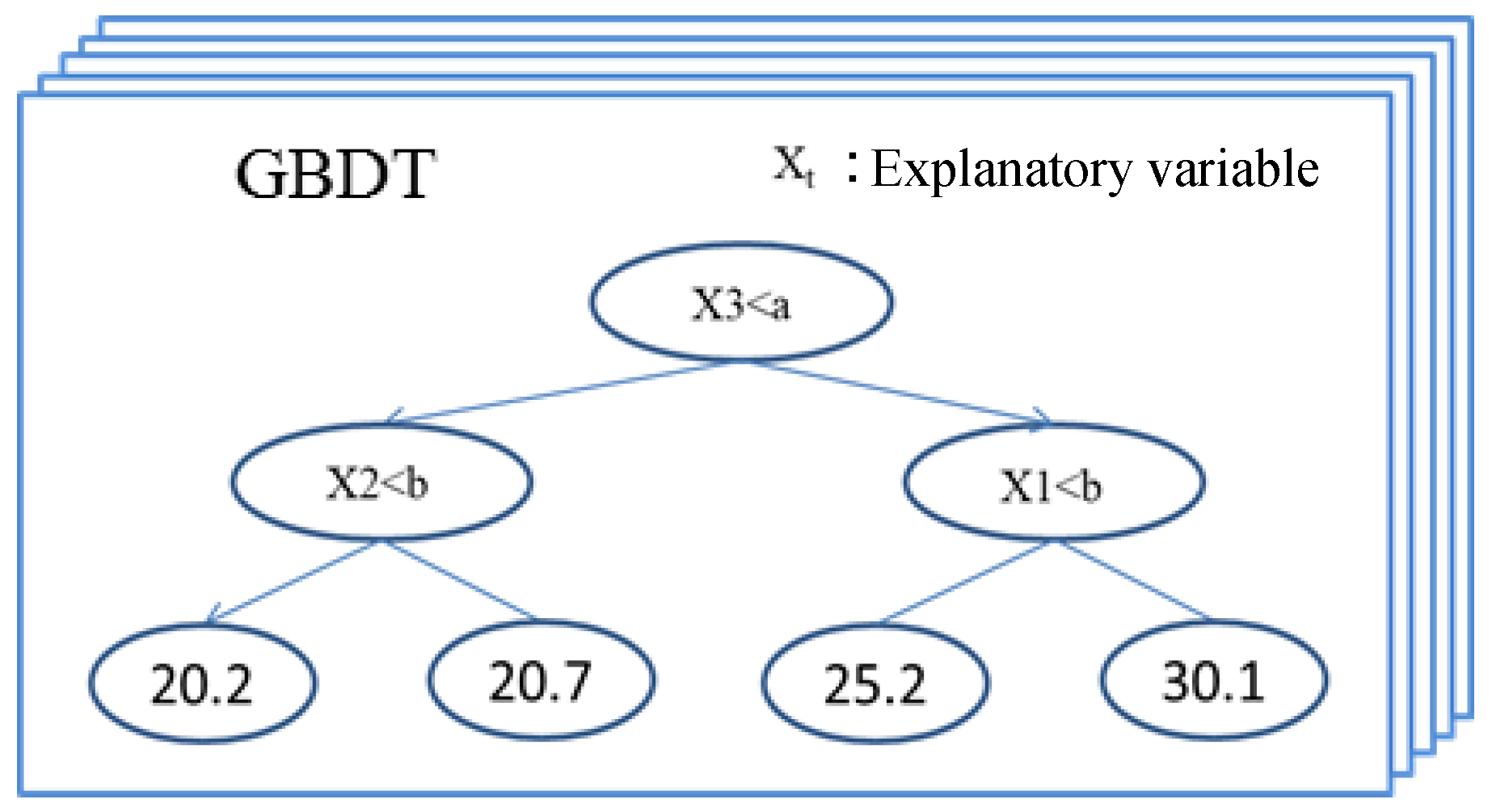
| 2 | Gradient-boosting decision tree (GBDT) |
| 3 | State-space model |
| No. | Explanatory Variable |
|---|---|
| 1 | CRAC cooling capacity |
| 2 | Outside-air temperature |
| 3 | Power consumption of each rack |
| Method | Evaluation Index | |||
|---|---|---|---|---|
| R | Correct-Answer Rate | RMSE | Max Peak Error | |
| Linear regression | 0.34 | 0.86 | 0.36 | 0.97 |
| GBDT | 0.81 | 0.99 | 0.11 | 1.07 |
| State-space model | 0.94 | 0.99 | 0.10 | 1.04 |
| Method | Explanation |
|---|---|
| GBDT | As an ensemble learning method using decision trees, a prediction method used in regression and classification problems [33] |
| State-space model | Prediction method used for time-series problems [34] |
| 2017 | |||||
|---|---|---|---|---|---|
| May | June | July | August | September | October |
| Learning | Evaluation | ||||
| Learning | Evaluation | ||||
| Learning | Evaluation | ||||
| Learning | Evaluation | ||||
| Learning | Evaluation | ||||
| Method | Evaluation Index | |||
|---|---|---|---|---|
| R | Correct-Answer Rate | RMSE | Max Peak Error | |
| GBDT | 0.82 | 0.62 | 0.35 | 2.77 |
| State-space model | 0.98 | 0.99 | 0.14 | 2.20 |
| Explanatory Variable Used | RMSE |
|---|---|
| Without CRAC power consumption | 0.13 |
| Without CRAC COP | 0.13 |
| Without CRAC cooling capacity | 0.13 |
| Without return temperature of CRAC | 0.18 |
| Without supply temperature of CRAC | 0.13 |
| Without power consumption of entire server room | 0.13 |
| Without power consumption of each rack | 0.14 |
| Only CRAC power consumption | 0.22 |
| Only COP of CRAC | 0.21 |
| Only CRAC cooling capacity | 0.22 |
| Only return temperature of CRAC | 0.15 |
| Only supply temperature of CRAC | 0.21 |
| Only power consumption of entire server room | 0.22 |
| Only power consumption of each rack | 0.18 |
| (Reference) when all variables are used | 0.14 |
| Method | Evaluation Index | |||
|---|---|---|---|---|
| (1) R | (3) RMSE | (4) max peak error | (5) NMBE | |
| Linear regression | 0.82 | 1.00 | 4.75 | 0.61 |
| Decision tree | 0.85 | 0.61 | 3.11 | 1.00 |
| gbdt | 0.88 | 0.56 | 2.56 | 1.37 |
| Method | 2017 | ||||||
|---|---|---|---|---|---|---|---|
| June | July | August | September | October | November | December | |
| Linear regression | 0.77 | 0.90 | 0.87 | 0.87 | 0.94 | 0.67 | 0.67 |
| Decision tree | 0.84 | 0.85 | 0.84 | 0.84 | 0.94 | 0.75 | 0.91 |
| GBDT | 0.90 | 0.89 | 0.89 | 0.88 | 0.95 | 0.70 | 0.94 |
| Learning Period No. | Explanatory Variable | Evaluation Period |
|---|---|---|
| 1 | Previous week | November and December, 2017 |
| 2 | Previous two weeks | |
| 3 | Previous three weeks | |
| 4 | Previous month | |
| 5 | Previous two months | |
| 6 | Previous three months | |
| 7 | Previous four months | |
| 8 | Previous five months | |
| 9 | Previous six months |
| Evaluation Index | Learning Period No. | ||||||||
|---|---|---|---|---|---|---|---|---|---|
| 9 | 8 | 7 | 6 | 5 | 4 | 3 | 2 | 1 | |
| Correlation coefficient | 0.67 | 0.53 | 0.60 | 0.59 | 0.52 | 0.70 | 0.74 | 0.52 | 0.51 |
| RMSE | 0.56 | 0.78 | 0.61 | 0.70 | 0.76 | 0.41 | 0.39 | 0.48 | 0.46 |
| Peak difference | 2.17 | 3.11 | 2.51 | 2.54 | 2.81 | 2.56 | 2.38 | 2.36 | 2.39 |
| Evaluation Index | Learning Period No. | ||||||||
|---|---|---|---|---|---|---|---|---|---|
| 9 | 8 | 7 | 6 | 5 | 4 | 3 | 2 | 1 | |
| Correlation coefficient | 0.94 | 0.94 | 0.95 | 0.95 | 0.94 | 0.94 | 0.94 | 0.94 | 0.88 |
| RMSE | 0.59 | 0.62 | 0.60 | 0.58 | 0.62 | 0.62 | 0.60 | 0.63 | 0.99 |
| Peak difference | 1.36 | 1.31 | 1.61 | 1.64 | 1.96 | 2.16 | 2.11 | 1.90 | 1.64 |
| Method | Evaluation Index | |||
|---|---|---|---|---|
| R | Correct-Answer Rate | RMSE | Max Peak Error | |
| State-space model | 0.99 | 0.98 | 0.14 | 2.37 |
| Method | Evaluation Index | ||
|---|---|---|---|
| R | RMSE | Max Peak Error | |
| GBDT | 0.91 | 0.26 | 0.49 |
| Rack No | Calculation Results | Max Measured Value | Error (Max Measured Value—Calculation Results) | Average Measured Value | Error (Average Measured Value—Calculation Results) |
|---|---|---|---|---|---|
| A1 | 30.36 | 32.62 | 2.26 | 30.77 | 0.41 |
| A2 | 29.52 | 31.45 | 1.93 | 29.52 | −0.01 |
| A3 | 30.63 | 32.61 | 1.98 | 31.09 | 0.46 |
| A4 | 29.56 | 31.57 | 2.01 | 29.16 | −0.40 |
| A5 | 33.46 | 35.00 | 1.54 | 32.82 | −0.64 |
| A6 | 29.99 | 32.11 | 2.12 | 29.54 | −0.45 |
| A7 | 31.15 | 33.35 | 2.19 | 31.21 | 0.05 |
| B1 | 30.86 | 32.89 | 2.03 | 31.09 | 0.23 |
| B2 | 29.31 | 31.09 | 1.78 | 29.04 | −0.28 |
| B3 | 29.48 | 31.45 | 1.97 | 29.11 | −0.37 |
| B4 | 31.48 | 33.58 | 2.10 | 31.43 | −0.04 |
| B5 | 29.38 | 31.34 | 1.96 | 29.47 | 0.09 |
| B6 | 31.76 | 34.06 | 2.30 | 31.61 | −0.15 |
| B7 | 29.13 | 31.46 | 2.33 | 29.03 | −0.10 |
| C1 | 30.38 | 32.67 | 2.29 | 30.86 | 0.47 |
| C2 | 30.20 | 32.30 | 2.10 | 30.71 | 0.51 |
| C3 | 32.85 | 34.92 | 2.08 | 33.15 | 0.31 |
| C4 | 29.66 | 31.44 | 1.78 | 29.72 | 0.06 |
| C5 | 29.05 | 30.76 | 1.71 | 29.14 | 0.09 |
| C6 | 29.87 | 31.82 | 1.95 | 30.01 | 0.15 |
| C7 | 28.80 | 30.53 | 1.73 | 28.87 | 0.07 |
| D1 | 30.25 | 32.00 | 1.745 | 30.45 | 0.20 |
| D2 | 29.99 | 31.77 | 1.78 | 30.20 | 0.21 |
| D3 | 30.83 | 33.09 | 2.26 | 31.11 | 0.28 |
| D4 | 30.01 | 31.49 | 1.48 | 29.84 | −0.17 |
| D5 | 29.53 | 31.14 | 1.61 | 29.34 | −0.18 |
| D6 | 28.88 | 30.73 | 1.85 | 29.03 | 0.15 |
| D7 | 28.62 | 30.50 | 1.88 | 28.83 | 0.20 |
| Period | Points | Setting of CRAC Return Temperature | (Measured Value-Based Run) Sum of 706 Points |
|---|---|---|---|
| 21 November 2019–6 December 2019 | 706 | 30 °C | 49.15 kW |
| Period | Points | Setting of CRAC Return Temperature | (Measured Value-Based Run) Sum of 706 Points |
|---|---|---|---|
| 10 December 2019–12 December 2019 | 97 | 26 °C | −33.05kW |
| 12 December 2019–16 December 2019 | 193 | 24 °C | −37.76kW |
| 16 December 2019–18 December 2019 | 97 | 22 °C | −13.67kW |
| 18 December 2019–20 December 2019 | 92 | 20 °C | −126.97kW |
| 2017 | |||||||
|---|---|---|---|---|---|---|---|
| May | June | July | August | September | October | November | December |
| learning | evaluation | ||||||
| learning | evaluation | ||||||
| learning | evaluation | ||||||
| learning | evaluation | ||||||
| learning | evaluation | ||||||
| learning | evaluation | ||||||
| learning | evaluation | ||||||
| Learning Period | RMSE |
|---|---|
| 7 days before the evaluation period | 0.12 |
| 14 days before the evaluation period | 0.13 |
| 21 days before the evaluation period | 0.12 |
| 31 days before the evaluation period | 0.14 |
| 61 days before the evaluation period | 0.12 |
| 91 days before the evaluation period | 0.13 |
| Method | 2017 | ||||||
|---|---|---|---|---|---|---|---|
| June | July | August | September | October | November | December | |
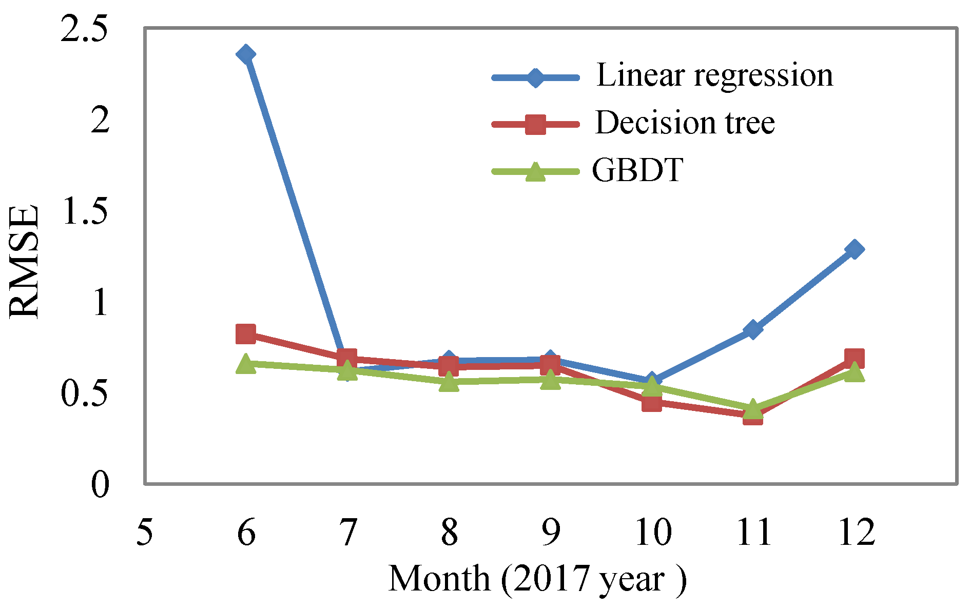
| Linear regression | 2.35 | 0.61 | 0.67 | 0.68 | 0.56 | 0.84 | 1.28 |
| Decision tree | 0.83 | 0.69 | 0.64 | 0.64 | 0.44 | 0.37 | 0.69 |
| GBDT | 0.66 | 0.62 | 0.56 | 0.57 | 0.54 | 0.41 | 0.61 |
| Method | 2017 | ||||||
|---|---|---|---|---|---|---|---|
| June | July | August | September | October | November | December | |
| Linear regression | 3.85 | 0.48 | 4.71 | 4.75 | 0.68 | 0.51 | 0.40 |
| Decision tree | 2.20 | 1.10 | 2.20 | 2.37 | 2.78 | 2.35 | 3.11 |
| GBDT | 1.64 | 0.75 | 2.22 | 2.20 | 1.14 | 2.56 | 2.16 |
| Method | 2017 | ||||||
|---|---|---|---|---|---|---|---|
| June | July | August | September | October | November | December | |
| Linear regression | 30.28 | 3.83 | −0.73 | 0.93 | 6.86 | 10.27 | 15.25 |
| Decision tree | −7.33 | 3.74 | −2.22 | −2.61 | −4.54 | 0.64 | 5.31 |
| GBDT | 6.78 | 3.69 | −2.14 | −2.44 | −7.73 | −1.52 | 7.29 |
© 2020 by the authors. Licensee MDPI, Basel, Switzerland. This article is an open access article distributed under the terms and conditions of the Creative Commons Attribution (CC BY) license (http://creativecommons.org/licenses/by/4.0/).
Share and Cite
Sasakura, K.; Aoki, T.; Komatsu, M.; Watanabe, T. A Temperature-Risk and Energy-Saving Evaluation Model for Supporting Energy-Saving Measures for Data Center Server Rooms. Energies 2020, 13, 5222. https://doi.org/10.3390/en13195222
Sasakura K, Aoki T, Komatsu M, Watanabe T. A Temperature-Risk and Energy-Saving Evaluation Model for Supporting Energy-Saving Measures for Data Center Server Rooms. Energies. 2020; 13(19):5222. https://doi.org/10.3390/en13195222
Chicago/Turabian StyleSasakura, Kosuke, Takeshi Aoki, Masayoshi Komatsu, and Takeshi Watanabe. 2020. "A Temperature-Risk and Energy-Saving Evaluation Model for Supporting Energy-Saving Measures for Data Center Server Rooms" Energies 13, no. 19: 5222. https://doi.org/10.3390/en13195222