Dynamic Response of an Inverted Pendulum System in Water under Parametric Excitations for Energy Harvesting: A Conceptual Approach

Abstract

In this paper, we have investigated the dynamic response, vibration control technique, and upright stability of an inverted pendulum system in an underwater environment in view point of a conceptual future wave energy harvesting system. The pendulum system is subjected to a parametrically excited input (used as a water wave) at its pivot point in the vertical direction for stabilization purposes. For the first time, a mathematical model for investigating the underwater dynamic response of an inverted pendulum system has been developed, considering the effect of hydrodynamic forces (like the drag force and the buoyancy force) acting on the system. The mathematical model of the system has been derived by applying the standard Lagrange equation. To obtain the approximate solution of the system, the averaging technique has been utilized. An open loop parametric excitation technique has been applied to stabilize the pendulum system at its upright unstable equilibrium position. Both (like the lower and the upper) stability borders have been shown for the responses of both pendulum systems in vacuum and water (viscously damped). Furthermore, stability regions for both cases are clearly drawn and analyzed. The results are illustrated through numerical simulations. Numerical simulation results concluded that: (i) The application of the parametric excitation control method in this article successfully stabilizes the newly developed system model in an underwater environment, (ii) there is a significant increase in the excitation amplitude in the stability region for the system in water versus in vacuum, and (iii) the stability region for the system in vacuum is wider than that in water.

1. Introduction

Global climate changes are rapidly transforming into more fatal and complex environmental disasters, happening all around the world. Abundant emission of hazardous gases form coal fired energy plants is one such kind of severe climate change. That is why the world energy paradigm is shifting from existing hazardous gas emission energy plant to finding new renewable and clean energy sources (such as photo-voltaic solar cells, nuclear energy, and ocean energy, etc.). The basic aim of this research article is to propose an initial concept related to energy harvesting from water waves devices. Moreover, this study has potential benefits in the field of underwater under-actuated robotic arm system.

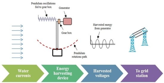
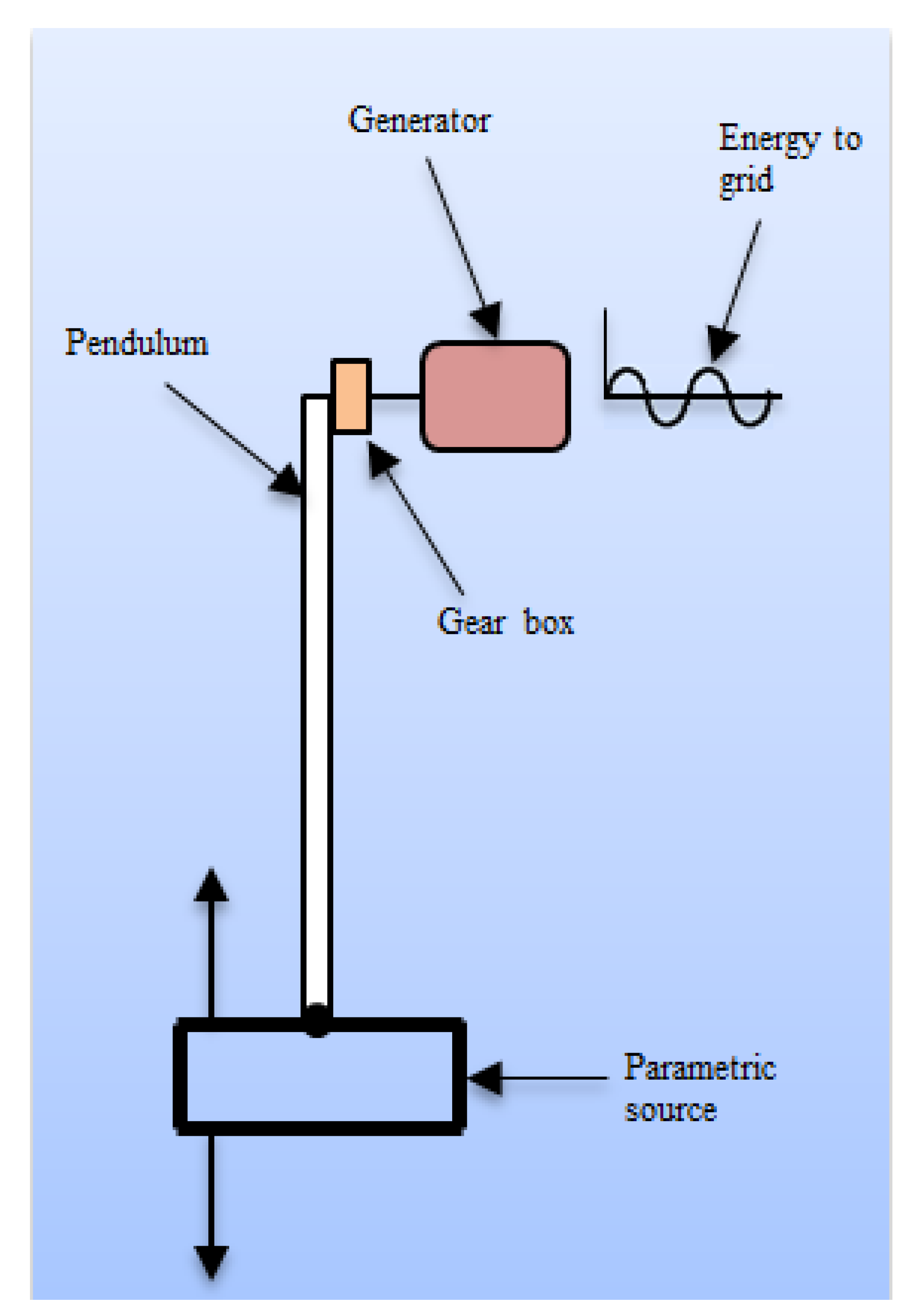
In this article, the dynamic response characteristics of an inverted pendulum system in viewpoint of a future wave energy harvesting device in an underwater environment are discussed. The problems associated with the dynamic response and parametric excitation control of the pendulum system are also addressed. Simple water waves are simulated through the concept of parametric excitations. Parametric excitation phenomena are widely used in the control design of various mechanical and electrical dynamical systems. Moreover, nowadays, parametrically excited pendulum systems are getting a huge attention in the development of wave energy converters and in various kind of energy harvesting devices. It is believed that wave energy can be successfully harvested if pivot point of an inverted pendulum system oscillates at a constant speed. This pivot point, oscillating with a constant speed in the horizontal direction will be attached to a generator. The attached generator will then produce electrical energy. Figure 1 shows the proposed conceptual schematic diagram of the wave energy harvesting system.

It is already known that the dynamic response behavior and stability control of a system in water is different than in vacuum [1]. The mathematical analysis and simulation of underwater systems can be very useful for understanding their physical characteristics. All underwater systems experience hydrodynamic forces during their operations, and these forces cause problems in their control and stabilization. That is why parametric excitations cannot be directly applied successfully in water without the development of a new model of an inverted pendulum system for stabilization purposes. Therefore, it is necessary first to obtain the dynamic model of a pendulum system while keeping in view the impact of the hydrodynamic forces on its surface. A pendulum-based system model has been used to show the response of water on a submerged body [2]. In addition, the dynamic response of a viscously damped and non-rotating single degree of freedom (DOF) pendulum system is investigated theoretically and experimentally. Several other works related to the development of dynamic models of different systems in water can be referred to in previous studies [3,4,5,6].

For at least one century, an inverted pendulum system has been considered as a benchmark system in designing, controlling, stabilizing, and testing of numerous nonlinear mechanical control applications, like boxingbots [4], segway [7], and an inverted pendulum cart system [8]. There are a number of standard control techniques that exist in the control engineering area, which have been tested on an inverted pendulum model prior to their implementation on the real systems [4,7,8,9,10,11]. For example, the design of an active stabilizing system for a single-track vehicle system was studied [12], and an intelligent control and balancing technique for a robotics system has been formulated [13]. A fuzzy controller has been suggested to solve the trajectory tracking problem of the inverted pendulum attached to a cart system [14], while a particle swarm optimization-based neural network controller has been designed for solving a real world unstable control challenge [15]. The mechanical systems mentioned above have been developed based on the dynamic design of pendulum systems in an open environment like air or vacuum. However, the work on the design and upright stability of a pendulum system in water (i.e., a viscously damped system) by introducing parametric excitations at its base has not yet been reported.

There already exist a number of scientific researches in the literature on the upright stability control of a statically unstable system through parametric excitations. Moreover, there are various control techniques which can be applied for control and stabilization purposes of an inverted pendulum system. Parametric excitation is one of the famous techniques that can be applied for such purposes. It is an open-loop control technique, and this technique does not require any state measurements of the plant. Initially, S. M. Meerkov had done some work on developing a general theory for parametrically excited systems [16]. He examined the effects of parametric excitations on the response of a controlled system by showing its stability and transient motion analysis. Furthermore, he introduced a control theory for a class of linear finite dimensional systems. Several approaches of parametrically excited systems are based on an averaging method. These approaches gained a greater attention in many other fields, including linear and non-linear control system theories. Since S. M. Meerkov’s publication on vibrational control systems, numerous other researchers have also done research in parametric excitations and stability of linear and non-linear dynamical systems by using an averaging technique, and without averaging technique [17,18,19,20,21,22].

It has already been discussed [16] that the parametric excitation control principle is based on the introduction of vibrations (like with zero mean value). Many researchers have used different dynamical systems and introduced the vibrational control system theory. In a previous study [23], the author has shown another method for parametric excitations of an under-actuated mechanical system; this method is the application of the geometric control technique in the differential geometry to determine necessary oscillatory inputs for stabilization and trajectory tracking. Numerical simulations are carried out to investigate stable domains of an inverted pendulum system [24]. The authors have shown that the loss of stability at larger value of amplitudes observed to follow Hopf bifurcation phenomena. They have further drawn a stability diagram for a pendulum system. A geometrical picture of an inverted pendulum behavior is given in a previous study [25]. Here, the reason behind the stability of a pendulum system through high frequency vibrations is examined. Averaging technique and vibrational control theory of mechanical systems were studied previously [26]. A link between averaging method and controllability theory is discussed by linking the concepts of averaged potential and symmetric product. The dynamic behavior of vertical structure of marine riser applications in the presence of hydrodynamic forces and under parametric excitations was studied previously [3]. The author has shown the dynamic response features of the system for undamped and damped cases, separately. His results illustrated that the effects of internal resonances due to the parametric excitations can be eliminated by considering the effect of hydrodynamic forces in the system dynamic model. Stabilization of upright vertical position of an inverted pendulum system by applying vibrational control is studied in another research [27]. A formula is also derived for the limit of region of stability of solutions of the Hill’s equation and with damping in the neighborhood of the zeroth natural frequency. A technique for determining the damping ratio of a parametric pendulum is presented in a report [28]. Pendulum rotations under parametric excitations from viewpoint of energy harvesting purpose are studied in another research [29]. As the uncontrolled system exhibits complex dynamics, thus the authors considered an added control torque method and obtained the optimal period-1 rotational motion for maximum energy harvesting. It was found that the limiting optimal solution gives about a quarter more energy harvesting than the uniform rotations generates. Moreover, the rotations of a parametrically excited pendulum system fitted on a floating support and were forced to move vertically under the influence of wave currents, and on the basis of a dedicated wave flume, laboratory experiments have been presented in [5]. Dynamics of the N-pendulum system and its application to wave energy are presented in a report [30] where numerical simulations were conducted for an experimental rig targeting under development to test the functionality of the concept and modeling the response of the N-pendulum. In one study [22], the authors investigated whether a parametric excitation control method can also be used for dynamic mechanical systems without the application of the averaging method. Furthermore, authors have shown that this control technique can also be used via stability plots and by using Mathieu equation. In another work [31], authors have presented a control approach for a parametrically excited pendulum system in view point of energy extraction from an oscillatory motion and sea currents. They have shown that the stable rotations can be obtained regardless of the forcing conditions and for every set of initial conditions. They have further stated that their control method can be used in designing the autonomous pendulum harvester devices.

Many authors have used different systematic and numerical techniques to determine the suitable conditions for stability and stable regions for pendulum systems. The stability border was calculated for an undamped case of an inverted pendulum by using the averaging method reported previously [32], whereas the stability border was calculated by using a numerical approach (i.e., approximate solution) [33]. The Floquet theory was used in another study [34] to determine the lower stability border in the closed form for a parametrically excited inverted pendulum system. The authors also computed the stability borders for both the undamped and viscously damped cases, and have shown that, at larger damping values, the forcing amplitude for a given frequency increases for the damped case as compared with an undamped case. The authors have investigated the dynamic response of a tilted parametric pendulum in a study [35] where they have plotted the control space diagram of major bifurcation loci for the inverted solutions of a pendulum system. Many authors have used parametric excitations for analyzing the dynamic responses and stability of marine risers [36,37,38]. More recently, a stability analysis of a deep water marine riser under the parametric excitations was studied [39].

To the best of our knowledge, there have been no studies found on the dynamic behavior and parametrically excited control of an inverted pendulum system in water in view point of wave energy harvesting purposes. This paper presents the dynamic response, upright control, and stability formulism of a pendulum system both in vacuum and in water, when subjected to a parametric excitation input in vertical direction at the support point for the purpose of stabilization. For the first time, a new dynamic model for investigating the underwater response of an inverted pendulum system has been developed, considering hydrodynamics forces. An averaging technique has been applied to obtain an approximate solution of the system. Furthermore, an open loop parametric excitation control technique has been applied to stabilize the pendulum at its upright unstable equilibrium position. We have plotted both the lower and upper stability borders of the pendulum system in vacuum as well as in water, which results in obtaining the corresponding stability regions of the pendulum system. The results are illustrated through numerical simulations. The simulation plots show the following observations: (i) The applied parametric excitation method proposed in this article successfully stabilized the newly developed pendulum system model in water, (ii) there is a significant increase in the excitation amplitude in the stability region for the system in water versus in vacuum, and (iii) the stability region for the system in vacuum is wider than that in water.

The rest of this article is summarized as follows. The physical system, problem formulation statement, and dynamic model of the inverted pendulum system in water are expressed in Section 2. Parametric excitation control of both systems is discussed in Section 3. Simulations, maximum energy harvesting, and various kinds of inverted pendulum systems responses in vacuum and in water are presented in Section 4. Finally, conclusions of this work are drawn in Section 5.

2. Statement of Problem Formulation

2.1. Pendulum System in Vacuum

The equation of motion of a simply undamped inverted pendulum in a vacuum environment with vertically driven support point oscillating with y(t) = μsin(ωt), forcing amplitude (μ), and the forcing frequency (ω) is given as:

$$\ddot{\theta }=\left(\frac{g}{l}-\frac{\mu {\omega }^2\sin (\omega t)}{l}\right)\sin \theta$$

(1)

where l is length of pendulum system and g is gravitational force. Since we are dealing with stabilization of vertically upright unstable equilibrium position of the inverted pendulum system, we linearized the nonlinear Equation (1) around θ = 0. By assuming that sinθ ≈ θ, then, the linearized equation obtained is given as:

$$\ddot{\theta }=\left(\frac{g}{l}-\frac{\mu {\omega }^2\sin (\omega t)}{l}\right)\theta$$

(2)

2.2. Pendulum System in Water

It is assumed that the underwater pendulum system is free to vibrate around its pivot point, and water is at rest. The underwater system experiences hydrodynamics forces acting on it relative to its motion, fluid viscosity, fluid velocity, and volume of the submerged body, etc. In such cases, the hydrodynamic forces cannot be neglected and create problems in controlling underwater systems. Such type of systems exhibits an example of viscously damped systems. The dynamics analysis and control of such underwater systems can be very useful to understand the physical behavior of these kinds of systems. For this purpose, we have studied and compared the stability and control performance of pendulum systems in both mediums (like vacuum and in water).

An inverted pendulum has two equilibrium points (0, π): zero is upright and unstable equilibrium position and 180 degree is downward stable equilibrium position. This work considers the model of pendulum system in an underwater environment when parametric excitations are applied vertically at its support point to control the system at its upright unstable position. The pendulum is directly attached to the vibrating base that produces periodic oscillation at a desired smaller amplitude and higher frequency. Figure 2a,b shows pendulums in vacuum and water, in which the hydrodynamic force and the buoyance force appear in Figure 2b. (x_o,y_o) are the coordinates of the mass, l is length of pendulum, θ(t) is deviation angle from the vertical line in radian, m is mass of inverted pendulum, F_B is buoyancy force, F_D is drag force, and μsin(ωt) is the parametric input at the support point.

Since the pendulum system is placed in water, that is why hydrodynamic forces will act on its surface. Buoyancy force F_B, drag force F_D have a significant effect on the dynamic response of the inverted pendulum system [40,41,42]. Thus, drag force, in-line with the fluid flow, can be obtained as follows:

$$F_D=\frac{1}{2}{C}_D{\rho }_w{A}_p{v}^2$$

(3)

where C_D is drag force coefficient, A_p is object’s dimensions, ν is relative velocity between the static fluid and mass, and ρ_w is the fluid density. In this article, fluid is not moving and only velocity of mass is taken into account. Additionally, buoyancy force can be obtained from the following equation as:

$$F_B={\rho }_w{V}_{r}g$$

(4)

where V_r is volume of inverted pendulum system. As whenever a body moves in a fluid, it also carries its own mass. This mass is defined as added mass (it is inertia added to a body, when the body moves some volume of surrounding fluid during its movements in a fluid), and this also gives an additional inertia to the system. This added mass is obtained from the following equation:

$$m_a=C_a{\rho }_w{V}_r$$

(5)

where C_a is called added mass coefficient.

The mathematical dynamic model of an inverted pendulum in water is obtained by applying the Lagrange method. The pendulum system in water is free to rotate around its vertical upright unstable position when parametric input is applied, thus resulting is a system that has one DOF. The deviation angle θ(t) is assumed to be the only generalized coordinate. Additionally, the kinetic energy (T) and potential energy (U) of the inverted pendulum system in water are derived from Figure 2b as follow:

$$T=\frac{1}{2}m{v}^2$$

(6)

$$U=\left(m_{r}g-F_B\right)y_o$$

(7)

where m_r is the mass of inverted pendulum in water, ν is velocity of the system, and F_B is buoyancy force acting on the pendulum system in an upward direction. Velocity v² represents a vector quantity and is defined as variation in the position of the system and is given as follows:

$$v^2=l^2\stackrel{.}{{\theta }^2}-2\mu l\omega \sin \theta \cos (\omega t)\stackrel{.}{\theta }+{\mu }^2{\omega }^2{\cos }^2(\omega t)$$

(8)

Now, the sum of all damping coefficients in conjunction with the movement of the pendulum system in water can be written in the form of a so-called dissipation energy (D) and is given by:

$$D=\frac{1}{2}{D}_{\theta }\stackrel{.}{{\theta }^2}$$

(9)

where D_θ is called as dissipative force coefficient and it is associated with the motion of the pendulum system in water. It is the sum of the viscous angular damping coefficient (Cv), mechanical damping (Cm), and electrical damping (Ce). As the drag force is the only opposing force that acts on the pendulum system under consideration, it can be represented as:

$$Q=sign(v)F_D$$

(10)

The drag force signal changes according to the angular movements of pendulum system [2]. If the angular movement is in clockwise direction, then the drag force signal is positive, otherwise it will appears as negative. The equation of motion of an underwater inverted pendulum system can be derived through the standard Lagrange method for a single DOF and a non-conservative system. Substituting Equations (6)–(10) in the Lagrange equation and performing the corresponding derivations yields the mathematical dynamic equation of a pendulum system in water including the expression for a parametric excitation input source as:

$$\ddot{\theta }=\frac{1}{m{l}^2}\left(\left(\left(m_{r}g-F_B\right)l-m\mu l{\omega }^2\sin (\omega t)\right)\sin \theta -D_{\theta }\stackrel{.}{\theta }+sign(v)F_D\right)$$

(11)

where m = m_r + m_a, μ is amplitude, ω is frequency of the oscillatory input system, and F_D, F_B, and D_θ are explained as in Equations (3), (4) and (8), respectively. The above nonlinear equation of an inverted pendulum system in water describes the dynamic behavior and motion characteristics of this system. The dynamics of such system can be segregated in two phases. The first is without, and the second is with the parametric excitation input, respectively.

3. Parametric Excitation Control

This section discusses the parametric excitation control method for a newly developed underwater (viscously damped) inverted pendulum system model through the averaging method. An inverted pendulum system shows the behavior of a second-order nonlinear dynamical system. The dynamic equation of the system and its corresponding approximate solution through the averaging method are discussed in the following section. For comparison purposes, the dynamic model of the pendulum system in vacuum is also presented.

3.1. Parametric Excitation Control of an Inverted Pendulum in Vacuum

As the exact solution of Equation (2) cannot be obtained directly, that is why we need to find an approximate solution of the system. By applying the averaging method on Equation (2), the averaged equation of the system with constant coefficients is obtained as follows:

$${\ddot{\theta }}_{av}=\left(\frac{g}{l}-\frac{{\mu }^2{\omega }^2}{2l^2}\right){\theta }_{av}$$

(12)

Equation (12) follows the reasoning that if the constant oscillations of lower excitation amplitude (i.e., smaller than the inverted pendulum’s length) and higher forcing frequency (i.e., larger than that of the systems natural frequency) are applied with the condition μ²ω² > 2gl, then, the induced vibrations asymptotically stabilize the averaged system in Equation (12) and the linearized inverted pendulum system in Equation (2). Hence, the lower stability border for the inverted pendulum system is given by the following inequality:

$${\mu }^2{\omega }^2-2gl>0$$

(13)

3.2. Parametric Excitation Control of Inverted Pendulum in Water

The linearized dynamic system model of the pendulum system by assuming sinθ ≈ θ, from Equation (11), can be written as:

$$\ddot{\theta }=\frac{1}{m{l}^2}\left(\left(\left(m_{r}g-F_B\right)l-m\mu l{\omega }^2\sin \left(\omega t\right)\right)\theta -D_{\theta }\stackrel{.}{\theta }+sign(v)F_D\right)$$

(14)

Now, applying the averaging method on Equation (14), the averaged equation of the system with constant coefficients obtained is as follows:

$${\ddot{\theta }}_{av}=\left(\frac{\left(m_{r}g-F_B\right)}{ml}-\frac{{\mu }^2{\omega }^2}{2l^2}\right){\theta }_{av}-\frac{D_{\theta }{\stackrel{.}{\theta }}_{av}}{m{l}^2}+sign(v)\frac{F_D}{m{l}^2}$$

(15)

Equation (15) tells that when the constant input of parametric excitations of lower amplitude and higher frequency are applied by satisfying the following inequality:

$${\mu }^2{\omega }^2>\raisebox{1ex}{$2(m_{r}g-F_B)l$}\!\left/ \!\raisebox{-1ex}{$m$}\right.$$

(16)

Then, the applied input vibrations asymptotically stabilize the averaged system given in (15) and linearized pendulum system in water given in (14). Hence, the lower stability border of an inverted pendulum system in water is given by the following inequality:

$${\mu }^2{\omega }^2-\raisebox{1ex}{$2(m_{r}g-F_B)l$}\!\left/ \!\raisebox{-1ex}{$m$}\right.>0$$

(17)

4. Numerical Simulation Results

This section presents the upright parametric excitation control, stability analysis, and the comparison of both un-damped system and inverted pendulum system (damped) in water, respectively, via simulations. The fourth-order Runge-Kutta (RK) method is used to compute numerical simulations results (MATLAB’s Simulink Toolbox was used for this purpose) of both non-linear inverted pendulum systems, given by Equations (1) and (11), respectively. Simulation values [1] used for the pendulum system are given in

Table 1. Values.

No.	Quantities	Values
1	Mass, mr (Kg)	0.165
2	Length, l (m)	1
3	Diameter, d (m)	0.01
4	Gravitational force, g (m/s2)	9.81
5	Coefficient of drag force, CD	1.28
6	Coefficient of added mass, Ca	2.0
7	Water density ρw, (Kg/m3)	1000

.

In the first phase, both inverted pendulum systems are displaced by 1 rad from their upright unstable upward equilibrium positions and without the application of any parametrically excited input. Figure 3 shows the time response and deviation (red line represents the upright equilibrium point of the pendulum systems) of angular displacements of inverted pendulum systems in vacuum (dash line), and in water (solid blue line) in the presence of hydrodynamics forces.

It can be observed that the angular displacement of both pendulum systems increases, and pendulums move away from their upright unstable positions, and finally become stable at their stable equilibrium position of 180 degrees. As we already know, the parametric excitation control method is only valid for certain bounded ranges of lower amplitudes and higher frequencies of the input oscillatory system as previously explained in [22,24,35,36]. That is why there exist two bounds for the stability of a pendulum system: A lower and an upper stability bound. Therefore, stability borders for both the systems in vacuum and in water are obtained from Equations (16) and (17) and are illustrated in Figure 4a,b. Figure 4a,b shows that if we choose any combination of input of a lower amplitude and higher frequency that falls within a stable region, that should stabilize both systems.

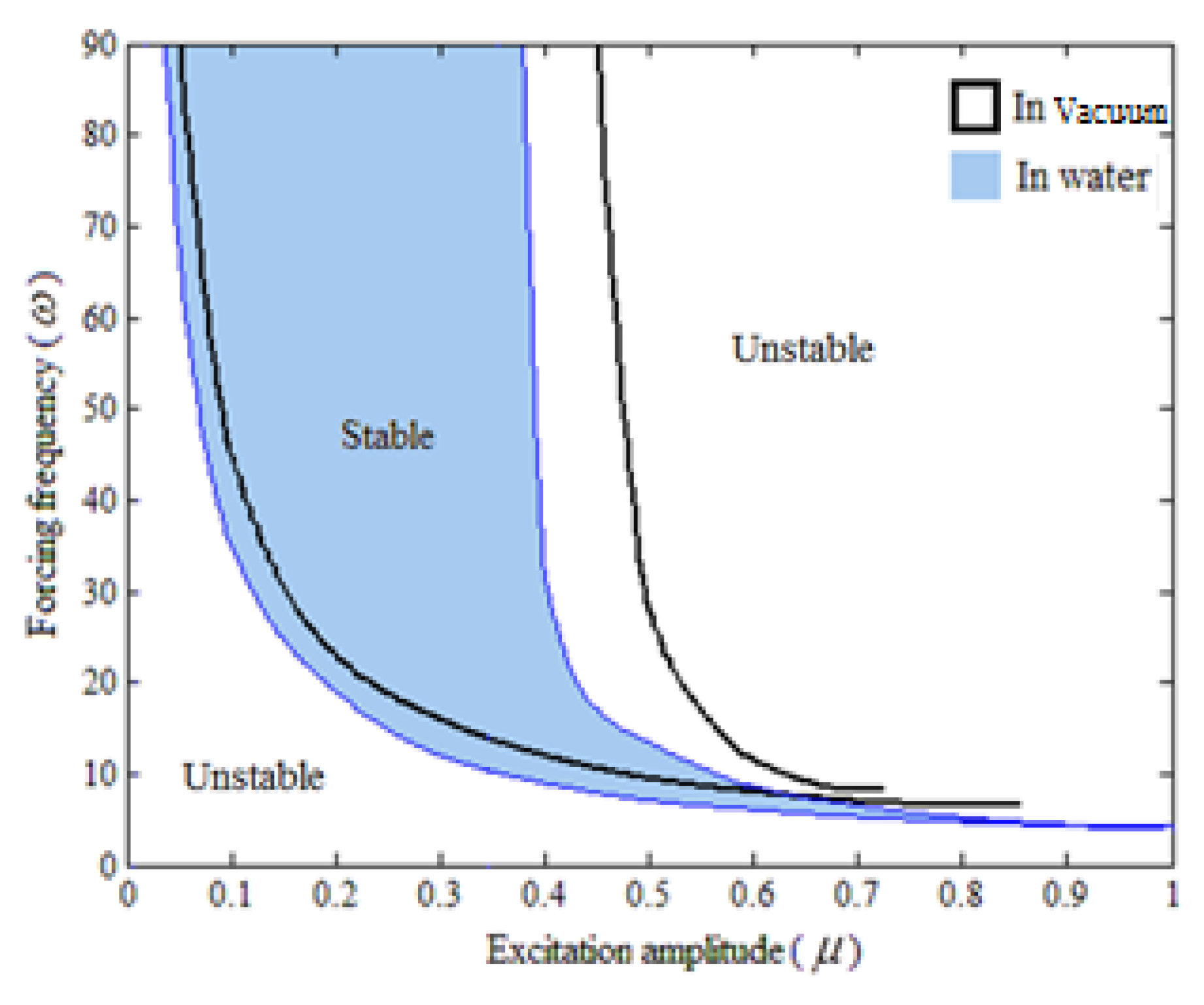
It is also shown that if we choose any combination of input of a lower amplitude and higher frequency that falls within the unstable regions, this will cause instability in both systems. Figure 5 illustrates the combined stability regions for both systems. It can be observed that the stability region for the system in vacuum is wider than for the system in water, and there is a significant decrease in the stability region for the inverted pendulum system in water.

The reason behind this difference is that the inverted pendulum system in an underwater environment is under the strong influence of hydrodynamics forces and represents a viscously damped system. There is also a significant increase in the excitation amplitude in the stability region for the system in water as compared with the pendulum system in vacuum. The above results are discussed for an undamped and damped pendulum cases in a previous study [35].

In the second phase, both the pendulum systems are initially taken away from their upright unstable position (zero rad) to 0.01 rad. Figure 6 shows a numerical simulation of an inverted pendulum system in vacuum for three different points with forcing frequencies of ω = 10, 14, and 20 rad/s, and excitation amplitudes of μ = 0.02, 0.04, and 0.06 m.

These points are illustrated in Figure 4a with black square dots. Figure 6a shows that the pendulum system is unstable in the lower unstable region, whereas Figure 6b illustrates that the system is stabilized around its upright unstable position in the stable region, and finally Figure 6c shows that the system is again unstable in the upper unstable region, and shows a rotating behavior. Figure 7 shows the numerical simulation of the pendulum system in water for different values of forcing frequencies, ω = 6.5, 12, and 40 rad/s, but with the same value of the excitation amplitude (like μ = 0.05 m).

These three points are illustrated in Figure 4b with blue circular dots. Figure 7a shows that the system is not stable around our targeted desired position, but it is showing an oscillatory behavior at another location. As mentioned in the literature, a pendulum system under parametric excitations would have more than one stability points (e.g., it may be showing stability around 45 degrees, etc.). However, our targeted stability point is only the upright position and best suited for energy harvesting purposes. Figure 7b illustrates that the system is stabilized around its upright unstable position in stable region, and finally Figure 7c shows that the system is unstable in the upper unstable region and finally becomes stable at 180 degrees. It can be observed that, in the underwater environment, the pendulum system is not exhibiting any rotational behavior in the unstable region. This is due to the strong effect of hydrodynamic forces.

Maximum Energy Harvesting

Figure 8a–l demonstrates the time responses of the parametrically controlled stable pendulum systems in vacuum and in water for several values of applied input of smaller amplitudes and higher frequencies. It is clearly evident from Figure 8a–f that the pendulum system is stable around its upright equilibrium position, but is continuously oscillating in case of vacuum medium. This means that these values of applied input of amplitude and frequency could not harvest maximum energy due to the fact that larger deviations from the equilibrium point could cause further vibrations in the entire system. It can be clearly observed from Figure 8g–l that the pendulum system is asymptotically stable around its upright equilibrium position in case of water which is a quite favorable condition for the operations of wave energy harvesting devices. This shows that these values of applied input of amplitude and frequency could continuously harvest the maximum amount of energy without safety hazards. Moreover, as mentioned in the literature, input values of applied amplitude and frequency for maximum energy harvesting might vary in case of complex water waves. As a result, up down movements of rectangular base attached at the base of the pendulum system could perform more complex motion profiles.

5. Conclusions

In this article, the phenomenon of dynamic stabilization and parametric excitation control for both the inverted pendulum systems (i.e., in vacuum and in water) is presented. Lagrangian approach has been used to derive the mathematical model for the study of dynamic analysis of a pendulum system, including the effect of hydrodynamic forces into account. The averaging method has been used to obtain the approximate solution for both systems. Moreover, the stability regions for both systems are illustrated through numerical simulations. The stability region graphs illustrate that any chosen combination of input of lower amplitude and higher frequency lying inside a stable region stabilizes and lying outside the stable region destabilizes both systems. The stability region graphs show that, for the pendulum system in water, the excitation amplitude for a specific forcing frequency increases as compared with the pendulum system in vacuum. The results illustrate that there is a significant increase in the excitation amplitude in the stability region for the underwater system as compared with the inverted pendulum system in vacuum. Furthermore, the entire system can be subjected to moving water disturbances and can be taken as a bench mark start point in designing wave energy harvesting devices in the future.

References

1. Shah, U.H.; Hong, K.-S. Input shaping control of a nuclear power plant’s fuel transport system. Nonlinear Dyn. 2014, 77, 1737–1748. [Google Scholar] [CrossRef]
2. Martins, D.; Silveira-Neto, A.; Steffen, V., Jr. A Pendulim-based model for fluid structure interaction analysis. Rev. Eng. Térmica 2007, 6, 76–83. [Google Scholar] [CrossRef]
3. Chatjigeorgiou, I. On the parametric excitation of vertical elastic slender structures and the effect of damping in marine applications. Appl. Ocean Res. 2004, 26, 23–33. [Google Scholar] [CrossRef]
4. Lee, G.H.; Lee, H.J.; Choi, H.J.; Jeon, H.J.; Jung, S. Application of mobile inverted pendulum systems to Boxingbots for a boxing game. In Proceedings of the 2009 IEEE/ASME International Conference on Advanced Intelligent Mechatronics, Singapore, 14–17 July 2009; pp. 963–968. [Google Scholar]
5. Lenci, S.; Brocchini, M.; Lorenzoni, C. Experimental rotations of a pendulum on water waves. J. Comput. Nonlin. Dyn. 2012, 7, 011007. [Google Scholar] [CrossRef]
6. Kopman, V.; Laut, J.; Acquaviva, F.; Rizzo, A.; Porfiri, M. Dynamic modeling of a robotic fish propelled by a compliant tail. IEEE J. Ocean Eng. 2014, 40, 209–221. [Google Scholar] [CrossRef]
7. Pathak, K.; Franch, J.; Agrawal, S.K. Velocity and position control of a wheeled inverted pendulum by partial feedback linearization. IEEE Trans. Robot. 2005, 21, 505–513. [Google Scholar] [CrossRef]
8. Gordillo, F.; Aracil, J. A new controller for the inverted pendulum on a cart. Int. J. Robust Nonlin. 2008, 18, 1607–1621. [Google Scholar] [CrossRef] [Green Version]
9. Spong, M.W. The swing up control problem for the acrobot. IEEE Control Syst. Mag. 1995, 15, 49–55. [Google Scholar]
10. Spong, M.W.; Corke, P.; Lozano, R. Nonlinear control of the reaction wheel pendulum. Automatica 2001, 37, 1845–1851. [Google Scholar] [CrossRef]
11. Jung, S.; Cho, H.-T.; Hsia, T.C. Neural network control for position tracking of a two-axis inverted pendulum system: Experimental studies. IEEE Trans. Neural Networ. 2007, 18, 1042–1048. [Google Scholar] [CrossRef]
12. Chu, T.-D.; Chen, C.-K. Design and implementation of model predictive control for a gyroscopic inverted pendulum. Appl. Sci. 2017, 7, 1272. [Google Scholar] [CrossRef] [Green Version]
13. Jin, S.; Ou, Y. A wheeled inverted pendulum learning stable and accurate control from demonstrations. Appl. Sci. 2019, 9, 5279. [Google Scholar] [CrossRef] [Green Version]
14. Llama, M.; Flores, A.; Garcia-Hernandez, R.; Santibañez, V. Heuristic global optimization of an adaptive fuzzy controller for the inverted pendulum system: Experimental comparison. Appl. Sci. 2020, 10, 6158. [Google Scholar] [CrossRef]
15. Lin, C.-J.; Lin, X.-Y.; Jhang, J.-Y. Unstable system control using an improved particle swarm optimization-based neural n etwork controller. Electronics 2019, 8, 1302. [Google Scholar] [CrossRef] [Green Version]
16. Meerkov, S. Principle of vibrational control: Theory and applications. IEEE Trans. Autom. Contr. 1980, 25, 755–762. [Google Scholar] [CrossRef]
17. Meerkov, S. Condition of vibrational stabilizability for a class of nonlinear systems. IEEE Trans. Autom. Contr. 1982, 27, 485–487. [Google Scholar] [CrossRef]
18. Bellman, R.; Bentsman, J.; Meerkov, S.M. Vibrational control of systems with Arrhenius dynamics. J. Math. Anal. Appl. 1983, 91, 152–191. [Google Scholar] [CrossRef] [Green Version]
19. Bellman, R.; Bentsman, J.; Meerkov, S. On vibrational stabilizability of nonlinear systems. J. Optim. Theory App. 1985, 46, 421–430. [Google Scholar] [CrossRef] [Green Version]
20. Bellman, R.; Bentsman, J.; Meerkov, S. Vibrational control of nonlinear systems: Vibrational stabilizability. IEEE Trans. Autom. Contr. 1986, 31, 710–716. [Google Scholar] [CrossRef]
21. Bellman, R.; Bentsman, J.; Meerkov, S. Vibrational control of nonlinear systems: Vibrational controllability and transient behavior. IEEE Trans. Autom. Contr. 1986, 31, 717–724. [Google Scholar] [CrossRef]
22. Berg, J.M.; Wickramasinghe, I.M. Vibrational control without averaging. Automatica 2015, 58, 72–81. [Google Scholar] [CrossRef]
23. Brockett, R.W. On the rectification of vibratory motion. Sens. Actuat. 1989, 20, 91–96. [Google Scholar] [CrossRef]
24. Blackburn, J.A.; Smith, H.; Grønbech-Jensen, N. Stability and Hopf bifurcations in an inverted pendulum. Am. J. Phys. 1992, 60, 903–908. [Google Scholar] [CrossRef]
25. Levi, M.; Weckesser, W. Stabilization of the inverted linearized pendulum by high frequency vibrations. SIAM Rev. 1995, 37, 219–223. [Google Scholar] [CrossRef]
26. Bullo, F. Averaging and vibrational control of mechanical systems. SIAM J. Control. Optim. 2002, 41, 542–562. [Google Scholar] [CrossRef] [Green Version]
27. Seyranian, A.; Seyranian, A. The stability of an inverted pendulum with a vibrating suspension point. J. Appl. Math. Mech. 2006, 70, 754–761. [Google Scholar] [CrossRef]
28. Horton, B.; Wiercigroch, M.; Xu, X. Transient tumbling chaos and damping identification for parametric pendulum. Phil. Trans. R. Soc. A 2008, 366, 767–784. [Google Scholar] [CrossRef]
29. Nandakumar, K.; Wiercigroch, M.; Chatterjee, A. Optimum energy extraction from rotational motion in a parametrically excited pendulum. Mech. Res. Commun. 2012, 43, 7–14. [Google Scholar] [CrossRef]
30. Yurchenko, D.; Alevras, P. Dynamics of the N-pendulum and its application to a wave energy converter concept. Int. J. Dyn. Contr. 2013, 1, 290–299. [Google Scholar] [CrossRef] [Green Version]
31. Reguera, F.; Dotti, F.E.; Machado, S.P. Rotation control of a parametrically excited pendulum by adjusting its length. Mech. Res. Commun. 2016, 72, 74–80. [Google Scholar] [CrossRef]
32. Landu, L.D.; Lifshitz, E.M. Mechanics; Pergamon Press: Oxford, UK, 1960; Volume 8. [Google Scholar]
33. Capecchi, D.; Bishop, S.R. Periodic oscillations and attracting basins for a parametrically excited pendulum. Int. J. Dyn. Stab. Syst. 1994, 9, 123–143. [Google Scholar] [CrossRef]
34. Erdos, G.; Singh, T. Stability of a parametrically excited damped inverted pendulum. J. Sound Vib. 1996, 198, 643–650. [Google Scholar] [CrossRef]
35. Sudor, D.J.; Bishop, S.R. Inverted dynamics of a tilted parametric pendulum. Eur. J. Mech. A Solids 1999, 18, 517–526. [Google Scholar] [CrossRef]
36. Hsu, C. The response of a parametrically excited hanging string in fluid. J. Sound Vib. 1975, 39, 305–316. [Google Scholar] [CrossRef]
37. Park, H.-I.; Jung, D.-H. A finite element method for dynamic analysis of long slender marine structures under combined parametric and forcing excitations. Ocean Eng. 2002, 29, 1313–1325. [Google Scholar] [CrossRef]
38. Prado, F.S.; Sakamoto, F.Y.; Mazzilli, C.E. An analysis of parametric instability of risers. Lat. Am. J. Solids Struct. 2014, 11, 348–368. [Google Scholar] [CrossRef] [Green Version]
39. Lou, M.; Hu, P.; Qi, X.; Li, H. Stability analysis of deepwater compliant vertical access riser about parametric excitation. Int. J. Nav. 2019, 11, 688–698. [Google Scholar] [CrossRef]
40. McLain, T.W. Modeling of Underwater Manipulator Hydrodynamics with Application to the Coordinated Control of an Arm/Vehicle System. Ph.D. Thesis, Department of Mechanical Engineering, Stanford University, Stanford, CA, USA, 1996. [Google Scholar]
41. Rahman, M.; Bhatta, D. Evaluation of added mass and damping coefficient of an oscillating circular cylinder. Appl. Math. Model. 1993, 17, 70–79. [Google Scholar] [CrossRef]
42. Lin, C.C.; Chen, R.C.; Li, T.L. Experimental determination of the hydrodynamic coefficients of an underwater manipulator. J. Robot. Syst. 1999, 16, 329–338. [Google Scholar] [CrossRef]
Figure 1. Proposed conceptual schematic diagram of the wave energy harvesting system.
Energies 13 05215 g001
Figure 2. Inverted pendulum systems with oscillatory input sources (a) in vacuum and (b) in water.
Energies 13 05215 g002
Figure 3. Time response of inverted pendulum systems without any oscillatory input.
Energies 13 05215 g003
Figure 4. Stability regions for inverted pendulum systems (a) in vacuum and (b) in water.
Energies 13 05215 g004
Figure 5. Combined stability regions for inverted pendulum systems.
Energies 13 05215 g005
Figure 6. Numerical simulation: (a) ω = 10, μ = 0.02; (b) ω = 14, μ = 0.04; and (c) ω = 20, μ = 0.06.
Energies 13 05215 g006
Figure 7. Numerical simulation: (a) ω = 6.5, μ = 0.05; (b) ω = 12, μ = 0.05; and (c) ω = 40, μ = 0.05.
Energies 13 05215 g007
Figure 8. Time response of inverted pendulum systems in vacuum ((a) ω = 25, μ = 0.02; (b) ω = 50, μ = 0.02; (c) ω = 25, μ = 0.03; (d) ω = 50, μ = 0.03; (e) ω = 25, μ = 0.04; (f) ω = 50, μ = 0.04), and water ((g) ω = 40, μ = 0.01; (h) ω = 60, μ = 0.01; (i) ω = 40, μ = 0.02; (j) ω = 60, μ = 0.02; (k) ω = 40, μ = 0.03; (l) ω = 60, μ = 0.03).
Energies 13 05215 g008