Article

A Novel Data-Energy Management Algorithm for Smart Transformers to Optimize the Total Load Demand in Smart Homes

1
Canada Excellence Research Chair Team, Concordia University, Montreal, QC H3G 1M8, Canada
2
Department of Electrical Engineering, Ecole de Technologie Superieure, Montreal, QC H3C 1K3, Canada
3
Mechanical Engineering Department, McGill University, Montreal, QC H3A 0G4, Canada
4
Department of Electrical Engineering, Faculty of Technology, University of Batna 2, Fesdis 05078, Batna, Algeria
*
Author to whom correspondence should be addressed.
Energies 2020, 13(18), 4984; https://doi.org/10.3390/en13184984
Submission received: 26 August 2020 / Revised: 14 September 2020 / Accepted: 21 September 2020 / Published: 22 September 2020
(This article belongs to the Special Issue Community Microgrids)

Abstract

:
The increased integration of Electric Vehicles (EVs) into the distribution network can create severe issues—especially when demand response programs and time-varying electricity prices are applied, EVs tend to charge during the off-peak time to minimize the electricity cost. Hence, another peak demand might be created, and other solutions are required. Many researchers tried to solve the problem; however, limitations exist because of the decentralized topology of the network. The system operator is not allowed to control the end-users’ load due to security and privacy issues. To overcome this situation, we propose a novel data-energy management algorithm on the transformer’s level that controls the power demand profiles of the householders and exchange energy between them without violating their privacy and security. Our method is compared to an existing one in the literature based on a decentralized control strategy. Simulations show that our approach has reduced the electricity cost of the end-users by 3%, increased the revenue of the system operator, and reduced techno-economic losses by 50% and 42%, respectively. Our strategy shows better performance even with a 100% penetration level of EVs on the network, in which it respects the network’s constraints and maintains the voltage within the recommended limits.

Graphical Abstract

1. Introduction

1.1. Literature Review

To mitigate the impact of the high penetration level of Electric Vehicles (EVs) on the distribution systems, advanced optimization algorithms and control strategies were developed including, but not limited, to (i) Centralized [1] (ii) Hierarchical [2], (iii) Multi-Agent [3], and (iv) Decentralized [4]. According to [5], due to privacy and security issues, the most used strategy to control the electrical appliances and devices at home is the decentralized control strategy. A home energy management system (HEMS) is deployed to control and schedule the power demand profile of the electrical devices. Internal optimization and control are required without any intervention or communication with any external agents [6]. Despite the usage of advanced optimization algorithms to obtain optimal scheduling of the loads at homes, the optimal solution may not participate in improving the total power demand profile on the Distribution Transformer (DT) and the Distribution Network (DN). This is due to the fact that most of the controllable loads, especially EVs, tend to consume much energy during low electricity prices; therefore, the DT capacities can be easily exceeded, and many issues might appear. Demand Response Programs (DRPs) were introduced to mitigate the impact of high power and energy demands during peak times and when there are lots of electricity burdens [7,8]. The DRPs can be categorized as, but not limited to, (i) price-based [9], (ii) incentive-based [4], (iii) power-based [6], and (iv) energy-based [4].
Home Energy Management Systems (HEMS) have been extensively studied in recent years, in which they have the ability to communicate with the Distribution System Operator (DSO) in order to receive the DRPs and electricity prices. An optimization algorithm is used to optimize and schedule the electrical loads with an objective to minimize the electricity cost at home. In paper [5], convex programming was considered for scheduling the electrical devices, which was more efficient and faster than other existing methods. The authors considered an EV, a photovoltaic system, and a battery storage system. However, the proposed control strategy cannot supply energy to the grid, and the objective function did not consider incentive programs. Hence, the method was not suitable to be considered for a larger scale. In [10], the authors considered the maintenance and generation cost of a wind turbine, photovoltaic, EV, and a battery storage system as the objective function. Despite an additional Renewable Energy Source (RES) being added to supply electricity to the home and grid, and despite advanced optimization techniques being used, such as the Taguchi method, results were not prominent for a larger scale. The main reason is that electrical loads tend to consume a lot of energy during periods when the electricity price is low. Therefore, peak demand could be formed during off-peak periods. To solve the problem, authors in [11] added more electrical loads to the schedule, and the problem was considered as a Mixed-Integer Linear Programming (MILP). In articles [10,11], a price-based demand response program is only used at home to minimize the electricity cost, which did not motivate householders to reduce their power demand in critical periods. To ameliorate the performance, especially from the viewpoint of the system operator, paper [4] considered both price- and incentive-based demand response programs. Results were better than [10,11]. However, the proposed method failed to limit the peak demand in some periods, and the transformer’s nameplate rating and power limit could be easily exceeded. To solve the problem, reference [6] introduced new power- and energy-based tariffs. The proposed DRPs were necessary to limit energy and power demand on the network. Despite the fact that many controlled devices were considered in the optimization model, a total load of all homes on the transformer might exceed the transformer capacity in some critical periods. Other new DRPs were introduced in paper [9], such as price- and power-limiting-based DRPs. The model responded to the contingencies on the network and controlled the electricity market price. However, the power limit of the transformer was not considered in the optimization model; hence, the transformer’s limit could be exceeded.
It is certain that many research papers worked on the integration of RES and EVs in order to improve their integration into the distribution network [8,12,13,14]. However, limitations always exist since the actual problem comes from the topology of the network’s infrastructure that is considered passive. Transformers are regarded as passive elements, in which their main role is to deliver electricity to the end-users and sometimes change the voltage rates. Hence, the existing topology of the distribution grid is a barrier and cannot mitigate the high penetration level of renewable energy technologies and EVs. From this place, many leading manufacturers such as ABB [15] and Siemens [16] developed a new generation of transformers named “Digital transformer”. This kind of transformer is equipped with sensors that measure, store, analyze, and generate real-time data of the operation of the transformer [17]. The data include, but are not limited to, the local weather data (e.g., humidity, ambient temperature), Global Positioning System (GPS) location, winding current and voltage, top-oil temperature, oil level, etc. Then, the transformer calculates some parameters, such as, but not limited to, the total harmonic distortion and the transformer’s lifetime. Both system operators and end-users are allowed to access the real-time data of the transformer; hence, they can better use the data to improve energy management and increase the efficiency of the network [16].
A further step into the smart grid was made by introducing the Solid-State Transformer (SST) [18]. Contrary to the existing coil-based transformer, the SST is a power-electronics-based transformer that converters AC-to-DC and DC-to-AC using different topologies. An SST has many functions such as (i) reduce the power fluctuations of the load, (ii) reduce power losses and harmonic distortion, (iii) mitigate the integration of Battery Storage System (BSS) and RES, (iv) improve the bidirectional power flow, (v) energy management of the DN, and (vi) voltage regulation [18]. Solid-state and digital transformers are promising technologies that improve the stability and efficiency of the network. However, they are not deployed due to several constraints, such as their high cost and some technical difficulties and limitations. Some studies have been carried out to manage the energy flow on the transformer level using these emerging technologies. Paper [19] studied the integration of SST to manage energy in a Photovoltaic-assisted Charging Station. The authors proposed a rule-based decision-making energy management system for SST to control the bi-directional power flow for supporting the real-time ancillary service. Authors in [20] developed a real-time energy management algorithm for a grid-connected charging park in an industrial and commercial workplace. Reference [21] proposed a high-power SST-based charging station for electric vehicles and discussed in-depth the application of solid-state transformer in the design of high-power electric vehicle charging stations. It is clear that the literature concentrates more on the integration of SST in electric vehicle parking lots and charging stations, in which centralized control strategies are used. Centralized control strategies can work for some end-users such as EV parking lots and charging stations, while they are not suitable for other end-users such as residential buildings and homes. Only decentralized control strategies can be used for such applications, although they have many limitations and barriers. From this place, it is crucial to develop a new control strategy that guarantees the independence of the consumers, increases their security, and protects their privacy, while respecting the constraints and limits on the distribution network. To the best of our knowledge, energy management systems for homes on the distribution network level using SST and DT, that satisfy both the system operator and the consumers, have not been studied yet, and need further investigation.

1.2. Contribution

To fill the gap in the literature and to overcome the existing power network topology limits, especially in the presence of EVs and RESs, we propose novel data-energy management algorithms on the Smart Transformer (ST) level to control the total load profile of each connected home. The novelty will be stated as follows:
  • It is the first algorithm that proposes a variable soft-constrained power profile limit for each home, in order to limit the power consumption. The limit is based on the classification of homes according to their average energy demand (from the lowest to the highest). This limit will satisfy the system operator by limiting the total power demand on the transformer, hence, reducing the techno-economic losses on the network.
  • This is the first algorithm that proposes decentralized demand response and incentive programs for each individual home. In another meaning, at a certain period, home 1 should not exceed 5 kW while, home 2 should not exceed 4 kW. If not, they will not benefit from the incentive programs.
  • This is the first algorithm that shares the unused energy between homes, which will maximize the load factor and minimize the power congestion on the network. Hence, the voltage profile is maintained within limits, and techno-economic losses are reduced.
  • Our strategy is designed to satisfy both end-users and the system operator, which will be a great advantage to be implemented. That is why it is necessary to define a new incentive program which encourages the end-users to use our strategy to minimize their electricity cost, and to maximize the profit of the system operator under certain constraints.
Moreover, the ST guarantees better privacy and security of the customers in which their private data are not sent to the system operator, while it is just used locally to manage energy on the transformer level. Our strategy is compared to an existing one in the literature (in which it used a conventional transformer). The comparison considers the technical and economic impact of both strategies on end-users, the transformer, the network, and the system operator.

1.3. Paper Organization

The organization of the paper is presented as follows. In Section 2, the proposed data-energy management system at the transformer level is presented and explained. Assumptions are listed in Section 3. The results are presented in Section 4. A conclusion is shown in Section 5, in which it summarizes the study and highlights the most important findings.

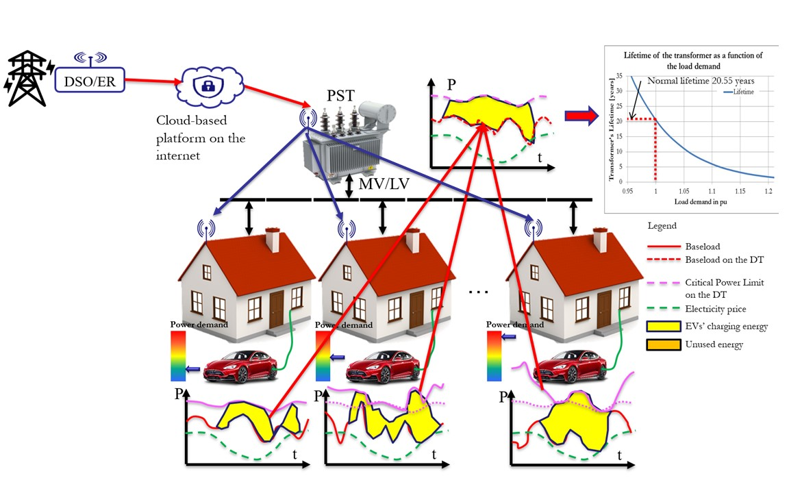
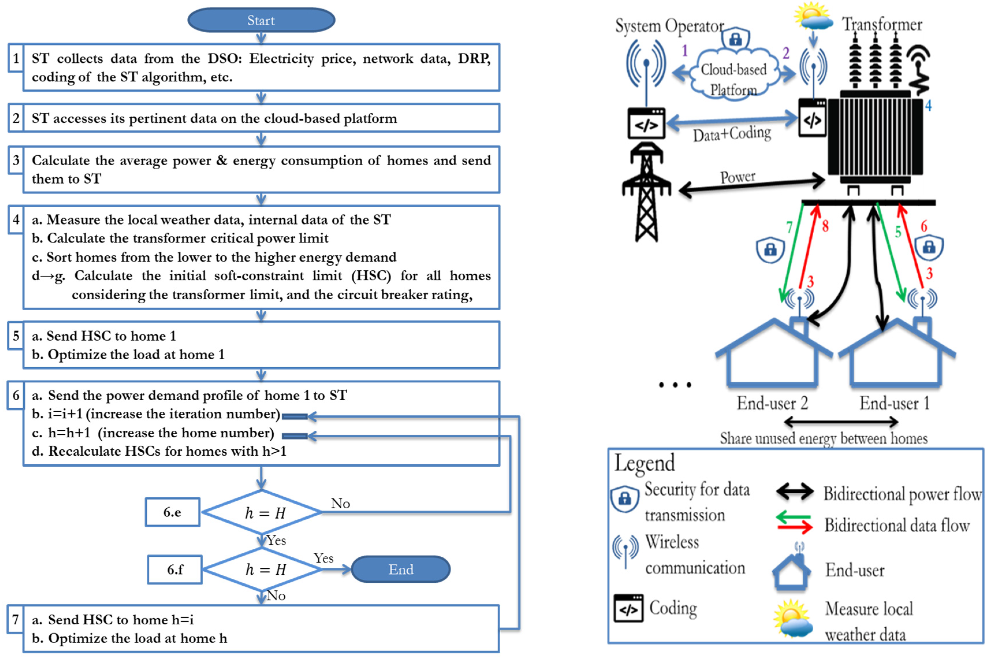
2. The Proposed Data-Energy Management Algorithm for the Smart Transformer

In this subsection, we propose a novel data-energy management algorithm on the transformer level that suggests a power soft-constraint limit for each home (HSC), in which the total power demand of all homes must respect the transformer critical power limit (e.g., 100 kVA). This limit is variable and depends on the power consumption profiles of all end-users. It allows the consumers to exchange the unused energy between them, which will increase their satisfaction while respecting the limits on the transformer. The transformer’s role is similar to the chief executive officer (CEO) of a company; it collects and analyzes data, takes decisions, and gives orders and tasks to the end-users to accomplish. The end-users are considered as the head of departments. They have the complete freedom to do whatever they want to, in a condition to perform their tasks within the specified period and constraints. In this way, the ST does not intervene directly with controlling and scheduling the electrical loads of the end-users. Moreover, the energy demand data of the consumers are manipulated internally between the transformer and the users, i.e., they are not sent to the system operator; hence, the security and privacy issues are resolved, which increases their satisfaction. The system operator’s role is to verify that the total load on the network respects the constraints and limits. From this place, the system operator only checks the status of the transformer and is not allowed to control the load of the consumers since the transformer can do it internally. The proposed algorithm is presented in different steps. Figure 1 shows a simplified schematic diagram of the proposed strategy. The following steps are considered:
StepDescription of the Flow Chart in Figure 1
1.ST receives data from the DSO, and the electricity retailer through the WIFI (as presented in Figure 2). Data are stored on a cloud-based platform using the most recent cybersecurity software (e.g., Global System for Mobile Communications (GSM) or Ethernet with the state-of-the-art cybersecurity). Data can be categorized as follows:
  • Householder’s data:
    Number of homes on the same smart transformer;
    Circuit breaker rates of each home;
    Number of phases for each home (e.g., single or three phases).
  • Cables’ data between the transformer and homes:
    Phase number, type, length, resistivity, inductivity, size.
  • Electricity Tariff: fixed price, progressive price, time-of-use, dynamic, real-time price, etc.;
  • Demand response and incentive programs;
  • Code for the smart transformer.
2.ST is assigned with a unique identification code in order to access data on the internet
3.
  • Active and reactive power demands of each electrical load at home are saved in the HEMS for a long period (i.e., one year);
  • The average apparent ( S h , t , d L o a d ) and active power ( P h , t , d L o a d ) consumptions are calculated as in Equation (1) for home “h” at instant “ t ” and day “d”, in which they are used to calculate the Home Soft-Constraint (HSC) limit as in Equations (5) and (11). HSC should be respected in order to guarantee that the total load on the ST will not violate its critical power limits and constraints;
  • Equation (2) calculates the average energy demand for a day;
  • The above mentioned data are received by the ST via local wireless communication between the ST and homes (e.g., WIFI, Long Range Wide-Area Network (LoRaWAN)). We are not using internet for security and privacy reasons. In this way, we also avoid any connection problems on the internet which might fail.
4.
  • Sensors in the ST collect weather and local data:
    Weather data, such as solar irradiance, wind speed, condition and alert, ambient temperature, humidity.
    ST internal data (in case it is a coil-based transformer):
    Top-oil temperature, winding current and voltage, and oil and moisture level.
    Other ST data: nameplate rating (e.g., 100 kVA), normal insulation life (e.g., 25 years), GPS location, number of phases, etc.
  • ST calculates the transformer’s critical power limit ( S t T C L ) as it is presented in [22].
    Energies 13 04984 i001
  • ST sorts and ranks homes from the lowest (h = 1) to the highest (h = H) average energy demand for a certain day.
    Energies 13 04984 i002
  • Equation (3) calculates the total homes aggregated circuit breaker rating ( S T o t a l C B ), where S h C B is the circuit breaker rate at home “ h ”. For example, S 1 C B = 5   kVA , S 2 C B = 7   kVA , S 3 C B = 9   kVA ,… S T o t a l C B = 5 + 7 + 9 +
  • Equation (4) calculates the soft constraint per unit ( α t ) at the home level. α t is in per unit and its has the same value for all homes on the same ST. Equation (5) calculates the soft-constraint apparent power ( S h , t H S C ) of each home. S h , t H S C can be different for each home; it is the result of multiplying α t by S h C B . If each home respects its soft-constraint limit ( S h , t H S C ), the transformer’s critical power limit will also be respected). In case the power demands at homes overpass their S h , t H S C , homes are not affected; however, the total load on the transformer may exceed its capacity. E h H S C is the energy soft-constraint limit at home in Equation (6).
    Example: consider four homes on an ST with the following data, we have to calculate α t and S h , t H S C .
    timeCircuit Breaker Capacity at home (kVA)Total Circuit Breaker Capacities of all homes (kVA)Transformer Rating Capacity (kVA)Transformer Real Power Limit (kVA)Soft constraint in per unitSoft constraint at home (kVA)
    S h , t H S C
    tH1H2H3H4 S T o t a l C B S t T C L α t H1H2H3H4
    12412264811075800.7317.458.7318.9134.91
    22412264811075700.6415.277.6416.5530.55
    32412264811075720.6515.717.8517.0231.42
    42412264811075770.7016.808.4018.2033.60
    52412264811075820.7517.898.9519.3835.78
    62412264811075680.6214.847.4216.0729.67
    Energies 13 04984 i003
    Energies 13 04984 i004
  • Energy demand may vary significantly from home to home for a certain period. Hence, S h , t H S C may decrease or increase depending on the home’s energy needs. Hence, calculating the optimal power soft-constraint limit for each home is necessary and is carried out by iteration considering the average energy demand. For this reason,   S h , t H S C is replaced by   S h , t H S C ( i ) as presented in Equation (8). The iteration number is represented by i . Starting from ( i = 1 ), S h , t H S C ( i ) . is iterated for all homes for t [ 1 , T ] . In Equation (9), β h , t ( i ) is the ratio of the power soft constraint at home to the transformer’s critical power limit. It is used for homes (h > 1), and it is used to calculate S h , t H S C ( i ) for homes h = 2 H . c h = 1 is a correction factor that is used to decrease or increase the power limit S h = 1 , t H S C ( i = 1 ) at home h = 1 depending on the actual energy demand. γ h , t is a factor that adjusts the HSC at home 1 in a way that E h L o a d , a v g E h H S C .
  • The first iterations of S h , t H S C ( i ) and β h , t ( i ) are sent to the home “h = 1”. These values are used as a constraint in the optimization model and algorithm. S h , t H S C ( i ) for all homes must be respected to respect the transformer’s power limit.
Energies 13 04984 i005
5.
  • S h , t H S C ( i ) and β h , t ( i ) are received by the Local Controller (LC) of home (h = 1).
  • Electrical loads at home “h = 1” are scheduled based on the optimal solution found by the LC. The algorithm for HEMS is set by a party such as end-user, DSO, or a specialized company, etc.
Energies 13 04984 i006
6.
  • After the optimization, ST receives P h , t L o a d   and S h , t L o a d from the LC, and calculates the unused energy in home 1. The unused energy is transmitted to other homes in order to use it and increase their soft-constraint power limit, which will help them to minimize their electricity cost and increase their demand if needed. The unused power and energy values are mentioned in the orange area of home 1 in the following figure:
    Energies 13 04984 i007
  • After receiving the information, ST increases i by 1 ( i = i + 1 ), e.g., i = 2 ; this means that a second iteration starts to calculate the soft-power constraints of all homes.
  • h is increased by 1 ( h = h + 1 ). For example, with h = 2 , the calculation of the P h , t L o a d   and S h , t L o a d starts from the second home to the last one.
  • In Equations (10) and (11), S h , t H S C ( i ) and β h , t ( i ) are recalculated for homes with h > 1 .
  • Compare h to H to verify if S h , t H S C ( i ) has changed for all homes starting from home h = h + 1 (e.g., h = 2 ), to h = H . If yes, set h = i (e.g., h = 2 ). If not, return to step 6.d.
  • Compare h to H for the second time. If h = H , it means that the calculation of S h , t H S C ( i ) , β h , t ( i ) and the optimization process has been completed for all homes. If not, data of the S h , t H S C ( i ) and β h , t ( i ) are sent to home h = i (e.g., h = 2) through steps 7, 9, 11, etc.
7.
  • Send S h , t H S C ( i ) and β h , t ( i ) to home h = i (e.g., h = 2).
    Energies 13 04984 i008
  • Optimize and schedule the controlled elements at home “h” as in step 5.b.
Energies 13 04984 i009
8.
  • Repeat the steps until h=H for the second comparison in step 6.f.
  • The final value of S h , t H S C and E h H S C are used as a soft-constraint at homes.
S h , t L o a d , a v g = d = 1 D S h , t , d L o a d D         ;         P h , t L o a d , a v g = d = 1 D P h , t , d L o a d D
E h L o a d , a v g = t T P h , t L o a d , a v g · Δ t
S T o t a l C B = h = 1 H S h C B
α t = S t T C L / S T o t a l C B
S h , t H S C = α t · S h C B
E h H S C = t T P h , t H S C
S h = 1 , t H S C ( i = 1 ) = α t · S h = 1 C B E h = 1 L o a d , a v g t T P h = 1 , t H S C c h = 1   f o r { h [ 1 , H ] t [ 1 , T ]
S h , t H S C ( i ) = α t · S h C B   f o r { h [ 1 , H ] t [ 1 , T ]
β h , t ( i ) = S h , t H S C ( i ) S t T C L γ h , t   f o r { h [ 1 , H ] t [ 1 , T ]
β h , t ( i ) = β h , t ( i 1 ) / h = i H β h , t ( i 1 )
S h , t H S C ( i ) = β h , t ( i ) ( S i 1 , t H S C ( i 1 ) S i 1 , t L o a d ) + S h , t H S C ( i 1 )

3. Assumptions for the Study

To validate our novel approach, a case study is chosen in Quebec, Canada. Generally, in Quebec, a transformer supplies ten homes with 200 A, single-phase (1 − φ) circuit breaker for each home. However, the proposed strategy could work no matter the number of homes, their circuit breaker ratings, or their load demands. The following data are provided by Hydro-Quebec Utility, reference [4], and other references for simulation purposes:
  • The baseload power and water consumption profiles at homes;
  • Real weather data such as solar irradiance and ambient temperature;
  • Real-time pricing is taken from reference [4] and presented in Figure 3;
  • Transformer data: 80 kVA, 1 − φ, 60 Hz, 11 kV/120 V;
  • Optimized elements at home are similar to reference [4]: 2 EVs, one BSS, one electric water heater, and one Photovoltaic (PV) system.
Our study is compared to reference [4]. Therefore, the same energy management system and optimization model are chosen for both studies. However, in [4] a conventional transformer is used, and energy management on the transformer level is not considered. Therefore, we carried out some modifications to the algorithm in which we added the power ( P h , t H S C ) and energy ( E h H S C ) soft-constraint limits at home, and we developed a new incentive program as presented in Table 1.
In Table 1, the homeowner gains 2.9 $/day and 2 $/day if the power and energy limits are respected, respectively. However, no additional tariffs are applicable if he does not respect these limits. This incentive program does not penalize users if they exceed the power and energy limits. However, each homeowner will save an amount of 1788.5 $/year (4.9 $/day × 365 day/year) if he does not exceed the limit during a complete year. This may cost the DSO lots of money for all end-users. However, DSO saves much more by reducing the techno-economic losses on the network. In this way, a win–win situation is settled between the householders and the DSO. The values of π P and π E are optimally chosen in a way to minimize the compensation of the DSO and increase the benefit of the end-users at the same time.
For validation purposes, our proposed method M2 is compared to the one (M1) in reference [4]. Mixed-Integer Nonlinear Programming (MINLP) is chosen to solve the optimization model for both methods in MATLAB R2016b. For the implementation of our strategy on a larger network, IEEE 123 node test feeder is chosen and solved in OpenDSS. Three different scenarios are considered:
  • Scenario 1: From the perspective of the customers using method 1, which is in favor of the consumers and not the system operator. The main goal of this scenario is to minimize the electricity cost at homes without considering the constraints on the network as in [4].
  • Scenario 2: From the perspective of the system operator using our proposed method 2 without considering our proposed incentive program. This method is called M2woIP (Method 2 without Incentive Program), which is in favor of the system operator and not the customer. In this scenario, the system operator gets the most benefits since it minimizes the techno-economic losses on the network while maximizing its revenue from the electricity bills.
  • Scenario 3: In this scenario, we tried to satisfy both end-users and the system operator, in which the end-user pays less than scenario 2 (sometimes even less than scenario 1), and at the same time, the system operator increases its revenue compared to scenario 1, which is due to the minimization of techno-economic losses on the transformer and the network. This scenario is called M2wIP (Method 2 with Incentive Program), in which we implement our proposed incentive program that encourages the users to adopt it and not to be fined in case they do not want to.
The above-mentioned scenarios are important and show how much the proposed method can encourage the system operator and the clients to adopt such strategies to increase their satisfaction, reduce their losses, and increase their revenue. In the following section, it becomes much clearer why we choose to study three different scenarios and which one is considered the best to be implemented.

4. Results and Discussions

In this section, both methods (M1 and M2) are studied, and techno-economic comparison is performed at home, on the transformer and the distribution network as presented in Table 2.

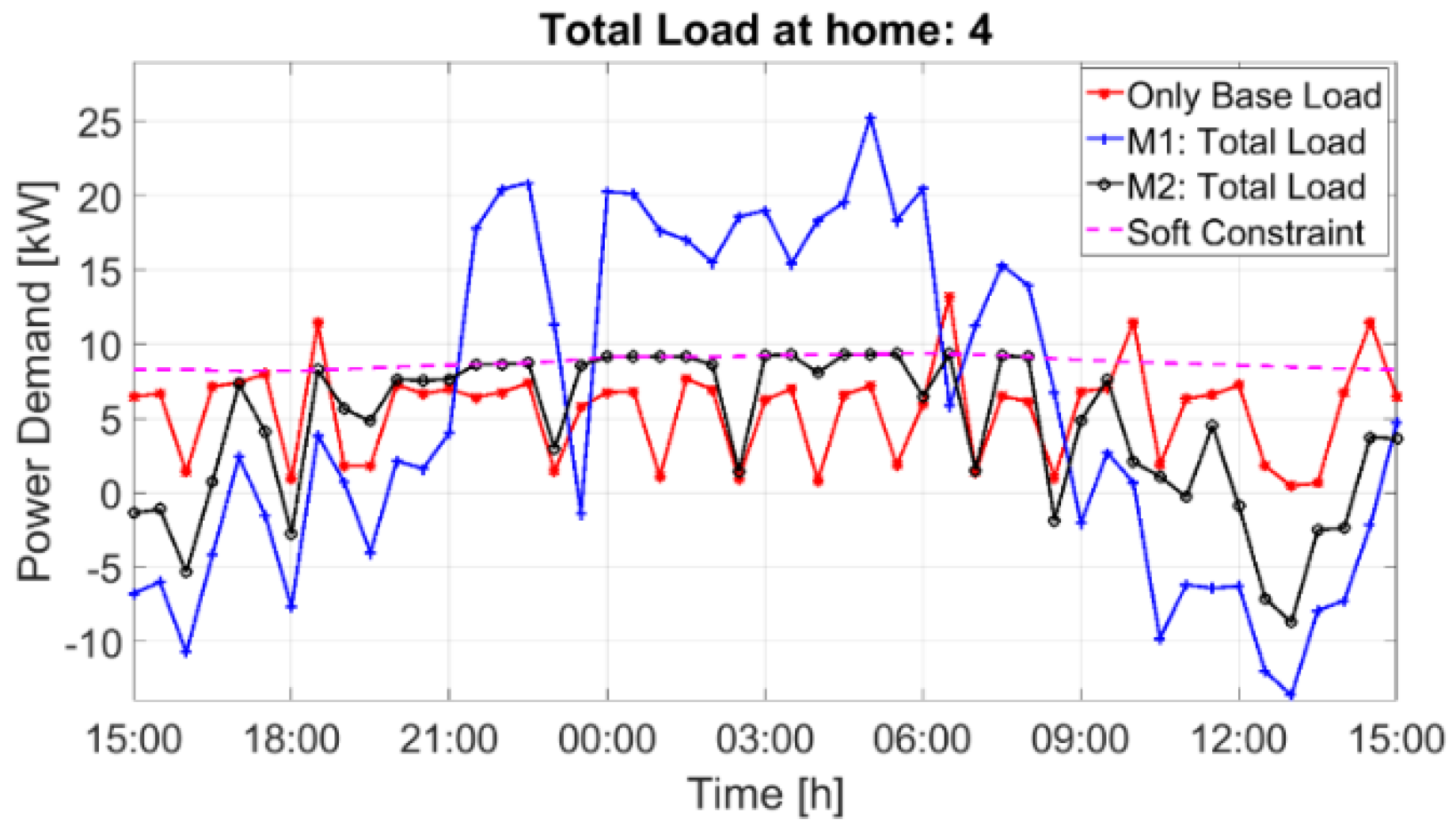
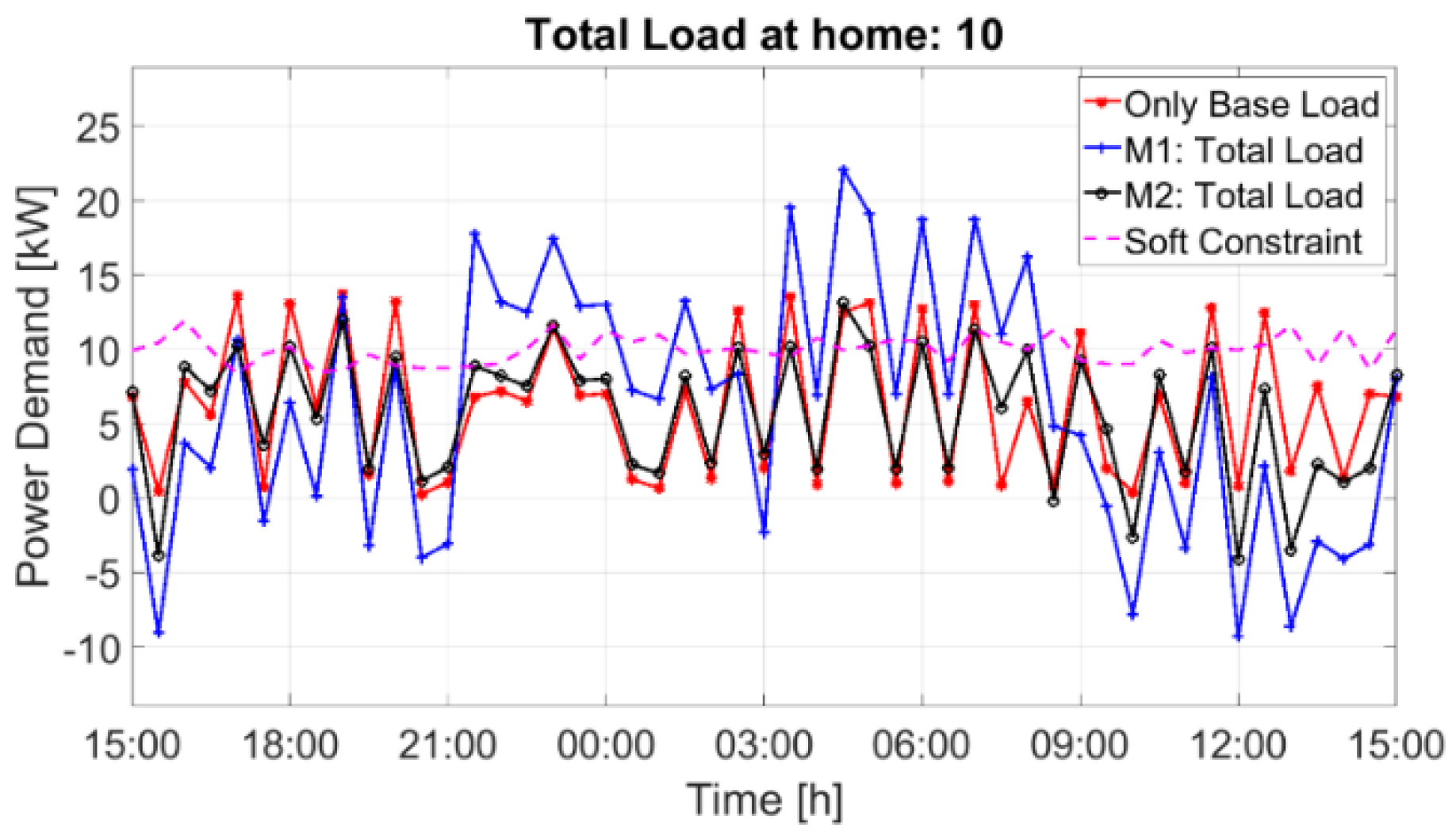
4.1. Impact on Power Consumption at Homes

This subsection aims at studying the impact of both methods on the total power consumption at homes. Two typical homes are considered in Figure 4 and Figure 5, in which Figure 4 represents homes 1, 2, 3, 4, 5, 7, 8, and 9 when the power consumption, using our method (M2), respects the soft-constraint limit (HSC), while Figure 5 represents homes 6 and 10 when M2 has slightly exceeded the soft-constraint limit. The case is different for M1, in which the power consumption using M1 at all homes has exceeded the HSC. In Figure 4, home 4 is studied. The red curve presents the power profile of the baseload, which cannot be optimized or controlled. For the case of M1 (blue curve), the power demand at home highly exceeds the HSC during low electricity price periods (between 21:00 and 09:00 as in Figure 3) for about 2.5 times (at 05:00 in Figure 4), which is considered very high. On the contrary, in periods when the electricity price is high, the power consumption appears negative (blue curve, between hours 15:00 and 21:00, and 09:00 and15:00), because the algorithm tries to minimize the electricity cost by injecting power to the grid from the EVs and the BSS.
On the other hand, for our method M2 (black curve), the HSC limit is respected by the power demand at home, and the charging period of the EVs might be extended, and could even charge during high electricity price due to the limit imposed by the HSC. Consequently, M2 has a higher electricity cost compared to M1, as presented in Figure 6 (blue columns compared to red columns).

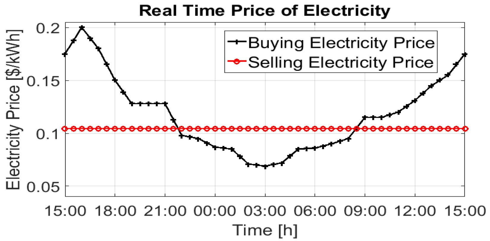
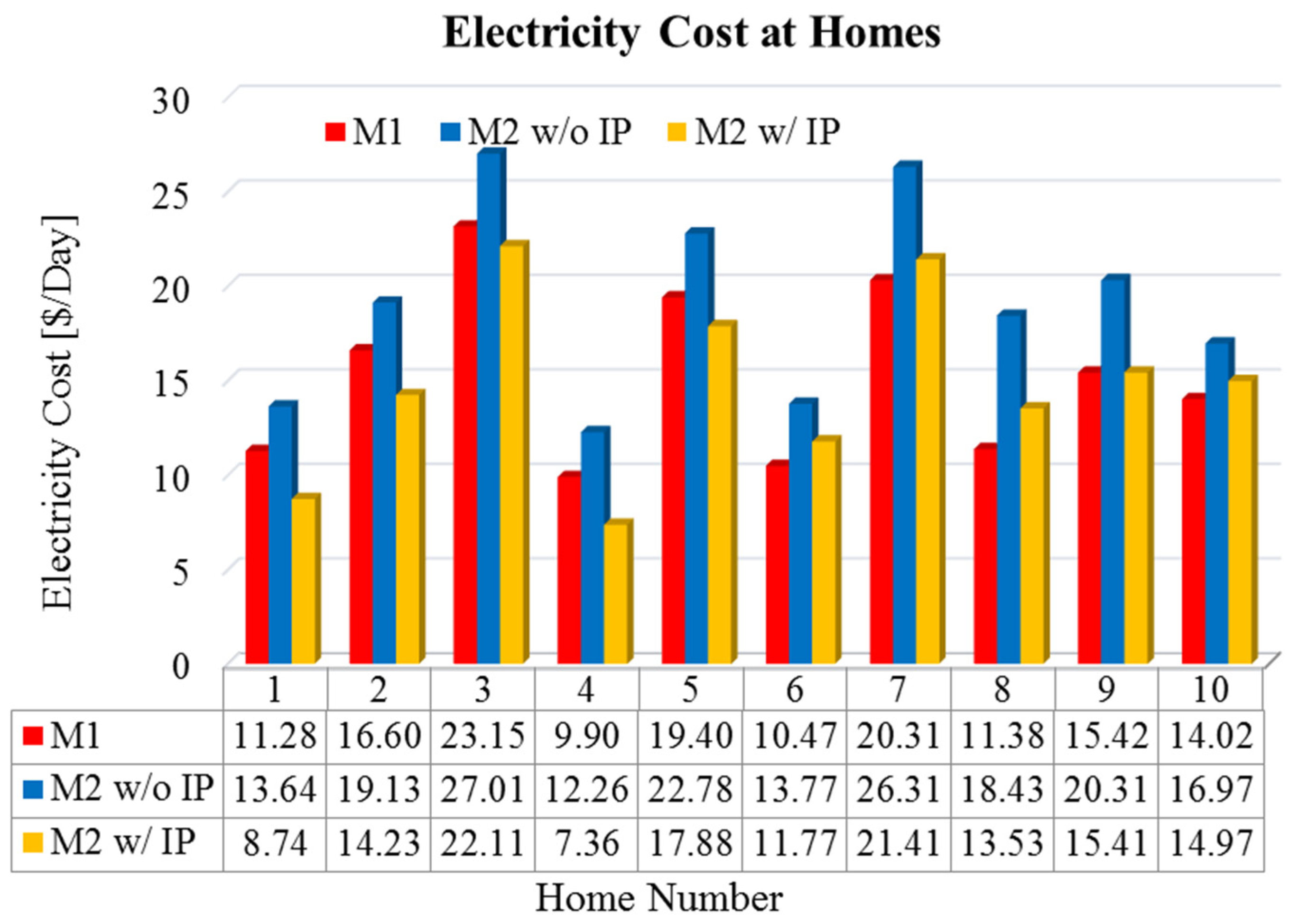
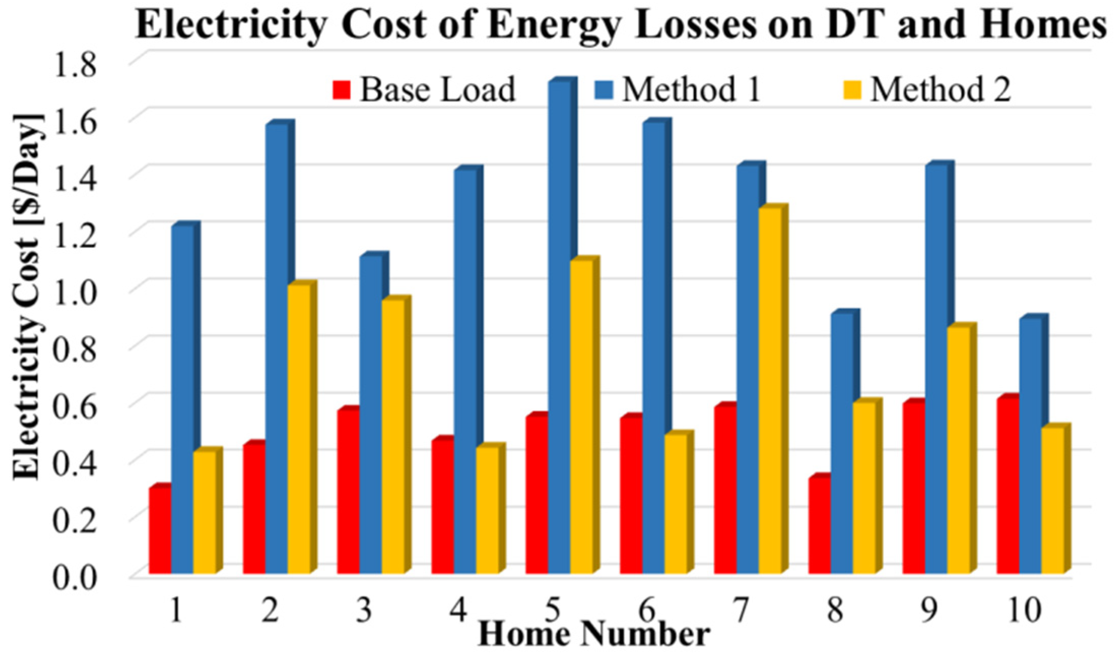
4.2. Economic Impact on the Electricity Cost at Homes

Figure 6 presents a comparison between the three methods:
  • M1 in red color;
  • M2 without our proposed incentive program (M2woIP) in blue color;
  • M2 with our proposed incentive program (M2wIP) in orange color (refer to Table 1).
M1 shows better results compared to M2woIP, which is very logical since M1 tries to minimize the electricity cost at home without considering the constraint HSC. M2woIP is perfect for the system operator and not for the end-user since his electricity cost at home becomes higher with the same energy consumption as in M1. Therefore, to increase the satisfaction factor of the householders, M2wIP is considered, and it gives better results than M2woIP, and sometimes better than M1, as can be seen for homes 1, 2, 3, 4, 5, and 9. The benefits of using M2wIP are stated as follows:
  • 2 $/day is deduced from the electricity bill of the householder if he respects the energy soft-constraint limit at home ( E h H S C );
  • 2.9 $/day is deduced if the householder respects the power soft-constraint limit at home ( P h , t H S C );
  • 4.9 $/day is deduced in case the householder is able to respect both energy and power soft-constraint limits;
  • 0 $/day is deduced in case the householder could not respect any limits (refer to Table 1).
In conclusion, M2wIP encourages the householders to adopt our strategy in order to reduce their electricity bill (sometimes even better than M1), while maintaining the stability of the network and protecting the transformers from overheating.

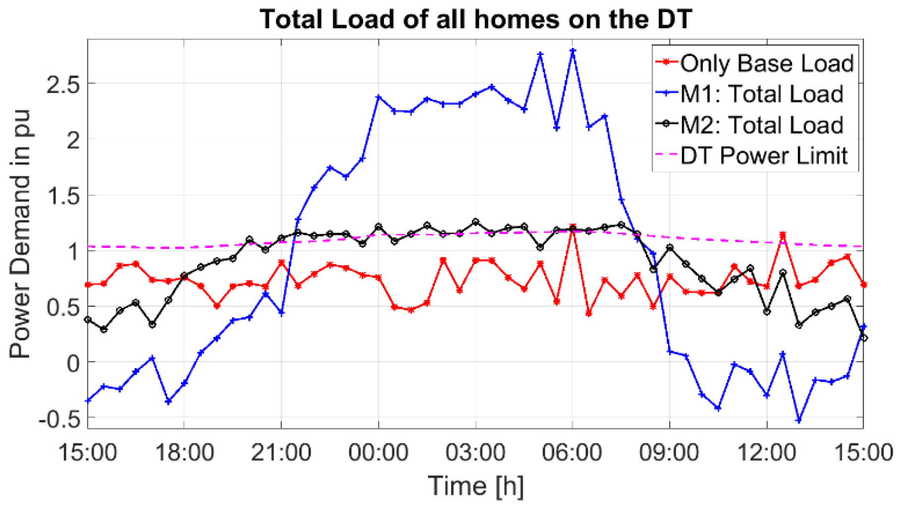
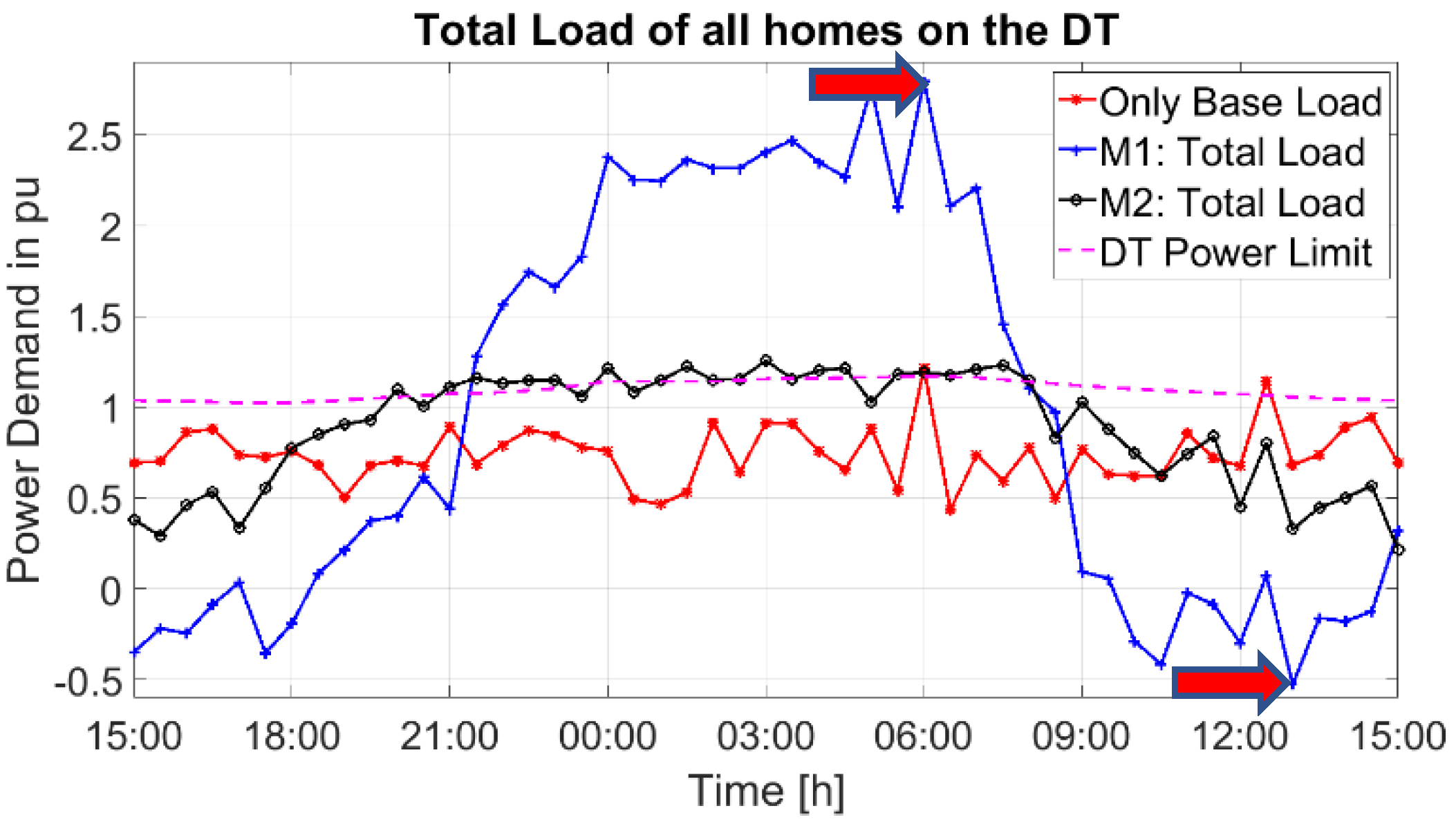
4.3. Technical Impact on the Distribution Transformer

Figure 7 and Figure 8 present the total power and voltage profiles of the transformer for three scenarios: (i) only baseload (red curve), (ii) M1 (blue curve), and (ii) M2 (black curve). The presence of two EVs, one BSS, and one EWH in each home puts lots of stress on the transformer. The total number of EVs is 20 for ten homes. Therefore, it is obvious for M1 (red curve) to exceed the critical power limit of the transformer since it does not consider our proposed power soft-constraint limit at homes. However, our method, M2, has increased the load factor and almost flattens the profile. Hence, M2 mitigates the impact on the transformer, reducing its loss of life. It also reduces the losses, and the voltage drops, as in Figure 8.
Please note that since some protection devices are used (such as circuit breakers and fuses), the mentioned peak demand for M1 on the transformer in Figure 7 might be lower. These devices will protect the transformer from very high overloading. However, protection devices can be activated, and circuit breakers might trip and leave the householders without electricity, and even blackouts on the network may happen. In this study, both methods, M1 and M2, are compared without considering the existence of the protection devices on the transformer in a goal to see their impact on the network without any interventions. Although, notably, if protection devices are activated, M1 risks reducing the lifetime of the transformer and causing brownout.

4.4. Economic Impact on the Distribution Transformer

After studying the technical impact, it is necessary to study the economic impact of both methods on the transformer and the network. Some definitions are necessary to be introduced at the beginning. In this paper, the Loss of Life during a day ( L O L D a y ) in Equation (12) is defined as the reduced time from the transformer’s lifetime during one day of operation in the presence of an electrical burden. L O L D a y is expressed by number of days. For example, L O L D a y = 3   d a y s means that one day of operation for a certain power demand profile is equivalent to 3 days of operations at the transformer full nameplate rating. Where L O L % is the percent loss of life of the transformer [23], L N is the transformer lifetime provided by the manufacturer in hours (e.g., L N = 180 , 000   h 20.55   years ) [23]. Sometimes, because of very high-power consumption during a day, the transformer may lose its total lifetime within one day of operation. Hence, the LOL per day cannot exceed its total lifetime. Therefore, it is necessary to limit its LOL to the maximum life expectancy of the transformer L N / 24 . For this purpose, the minimum between the percent loss of life per day and the total lifetime of the transformer is considered in order to guarantee the real values of the LOL per day.
L O L D a y = m i n ( ( L O L % 100 · L N 24 ) ; L N 24 )
In Equation (13), the transformer’s Remaining Lifetime ( R T D T ) is defined as the period in which the transformer can survive if the same power demand profile is applied every day. E.g., R T D T = 6000   days means that the transformer can survive 6000 days if it the same power demand profile is applied every day.
R T D T = L N L O L Day
Table 3 presents the results of the Loss of Life per day, the transformer’s remaining lifetime, and its benchmark depreciation cost per day. Regarding the baseload, the LOL per day is equal to 0.25, which is considered below the reference value “1”. It means that one day of operation at the baseload power profile is equal to 0.25 days of operation at the transformer’s full power capacity. Therefore, the remaining lifetime of the transformer is increased to 80.95 years (instead of 20.55 years), and the depreciation cost shows a negative value, which means that the DSO is saving 0.6 $/day because of the low power demand. However, the case is different for M1 and M2. As M1 has created a high peak demand during the day for a long period, the LOL per day is equal to the transformer lifetime 20.55 years (or 7500 days). In another meaning, the transformer lasts only for one day and ceases to function. Its benchmark depreciation cost is equal to the transformer’s cost (6000 $). Therefore, the DSO should change the transformer after one day of operation, which will cost millions and even billions of dollars for a large network. On the contrary, M2 shows a better performance, in which the LOL per day is reduced to 1.81 days for the same energy demand during a day (instead of 7500 for the case of M1). Therefore, the remaining lifetime of the transformer is increased to 11.35 years, and the benchmark depreciation cost becomes equal to 0.65 $/day.
Figure 9 and Figure 10 show the impact of both methods on the total energy losses and their cost on the DT and at homes during a day, respectively. M1 has the highest energy losses, while M2 shows better performance and has reduced the energy losses up to 71.4% (for home 4) and their cost by 69.2% (for home 6). Moreover, M2 has reduced the cost even below that of the baseload for homes 4, 6, and 10, which is considered a remarkable improvement. The reduction in energy losses increases the saving of the DSO since it is not paid by the end-users.

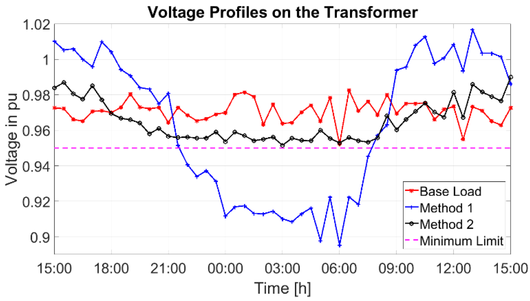
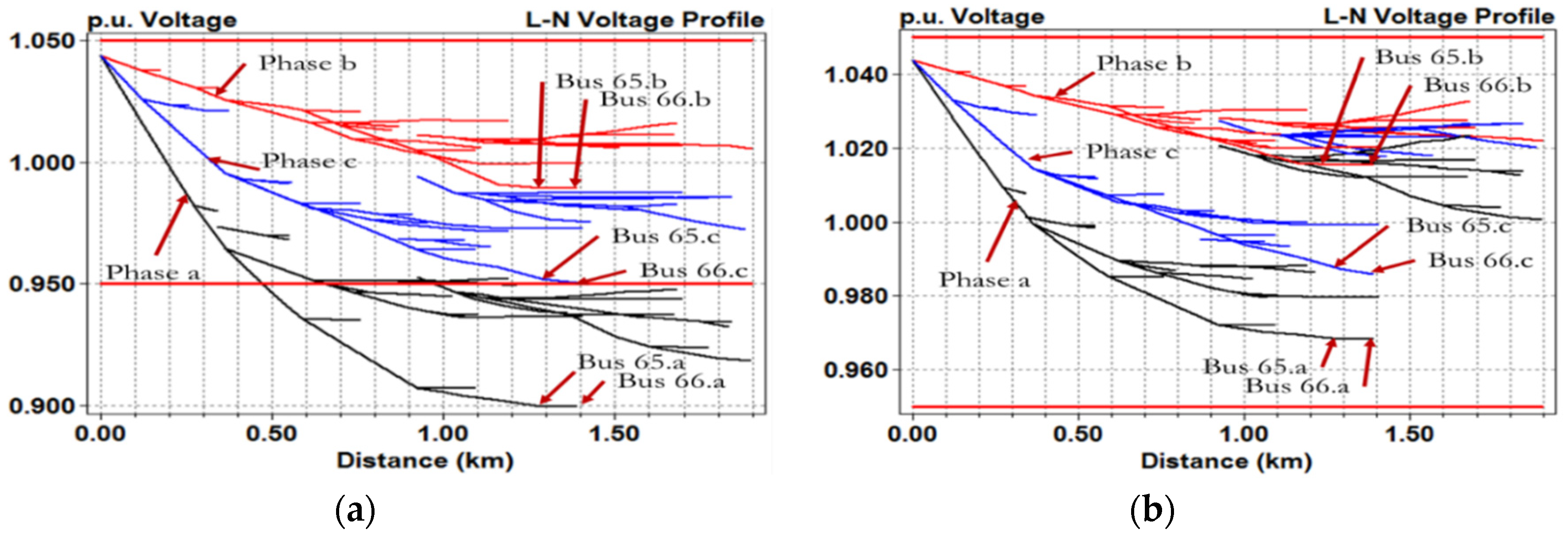
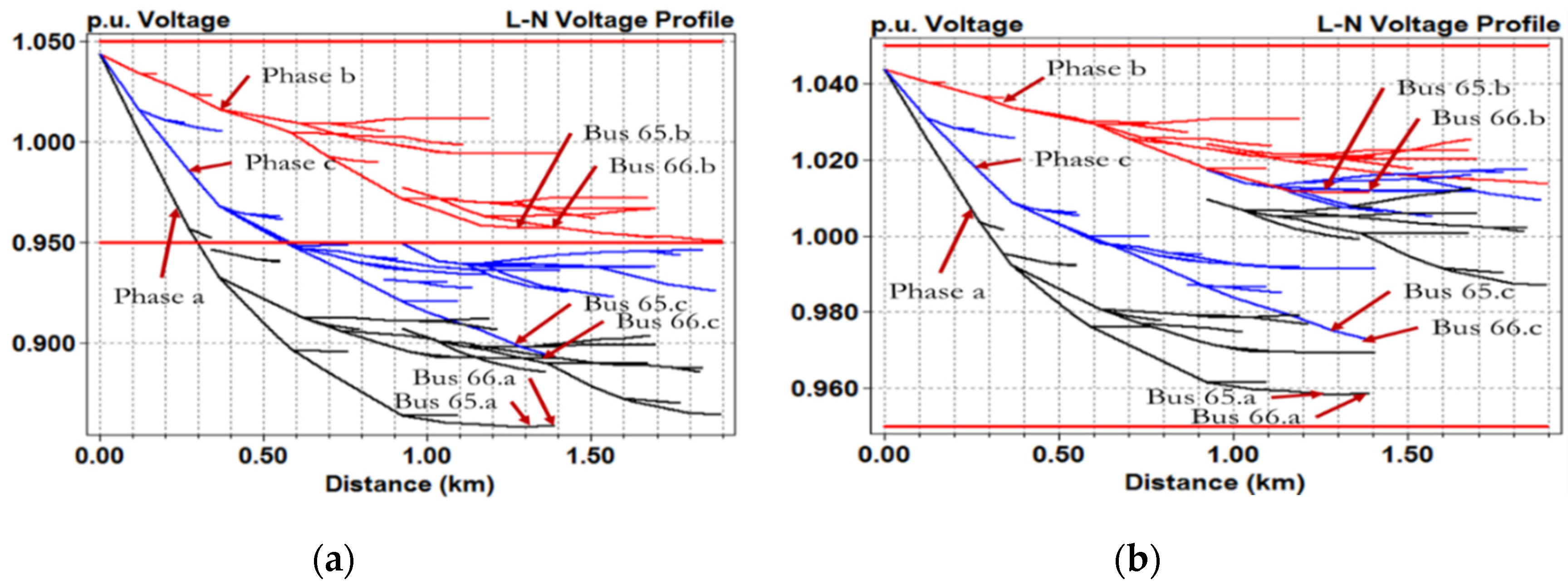
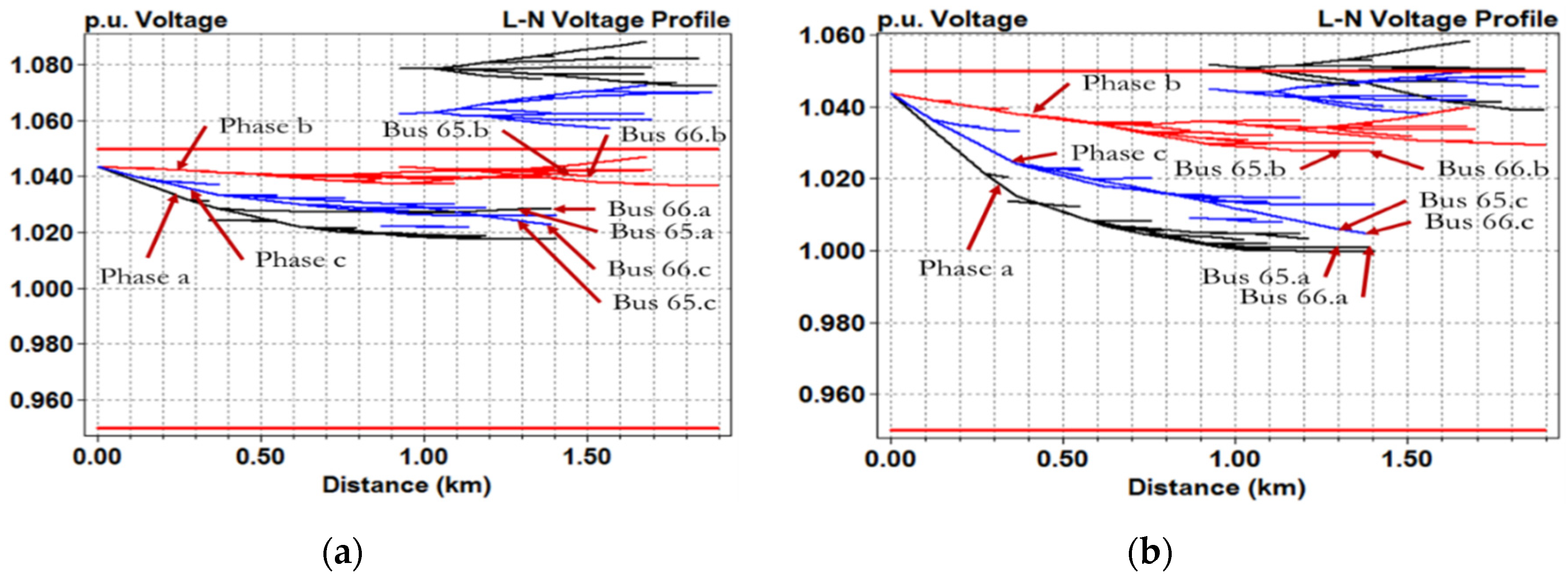
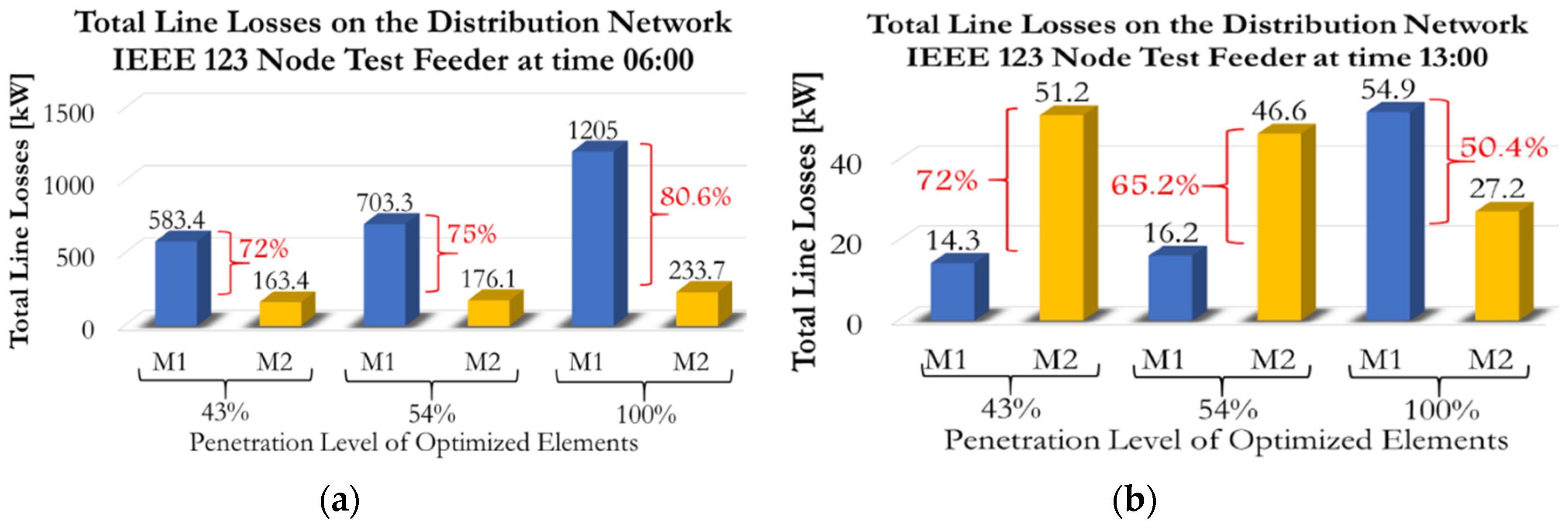
4.5. Technical Impact on the Network

In this subsection, the impact of both methods on a large distribution network is considered and studied. Voltage drop, power losses, and their cost are calculated for each point of the distribution network. To do so, some assumptions are necessary to be considered:
1-
OpenDSS is chosen as software to solve the power flow on the distribution network;
2-
Two particular hours are studied as in Figure 11, 06:00 and 13:00, in which the power demands using M1 attain their maximum and minimum values during a day, respectively;
3-
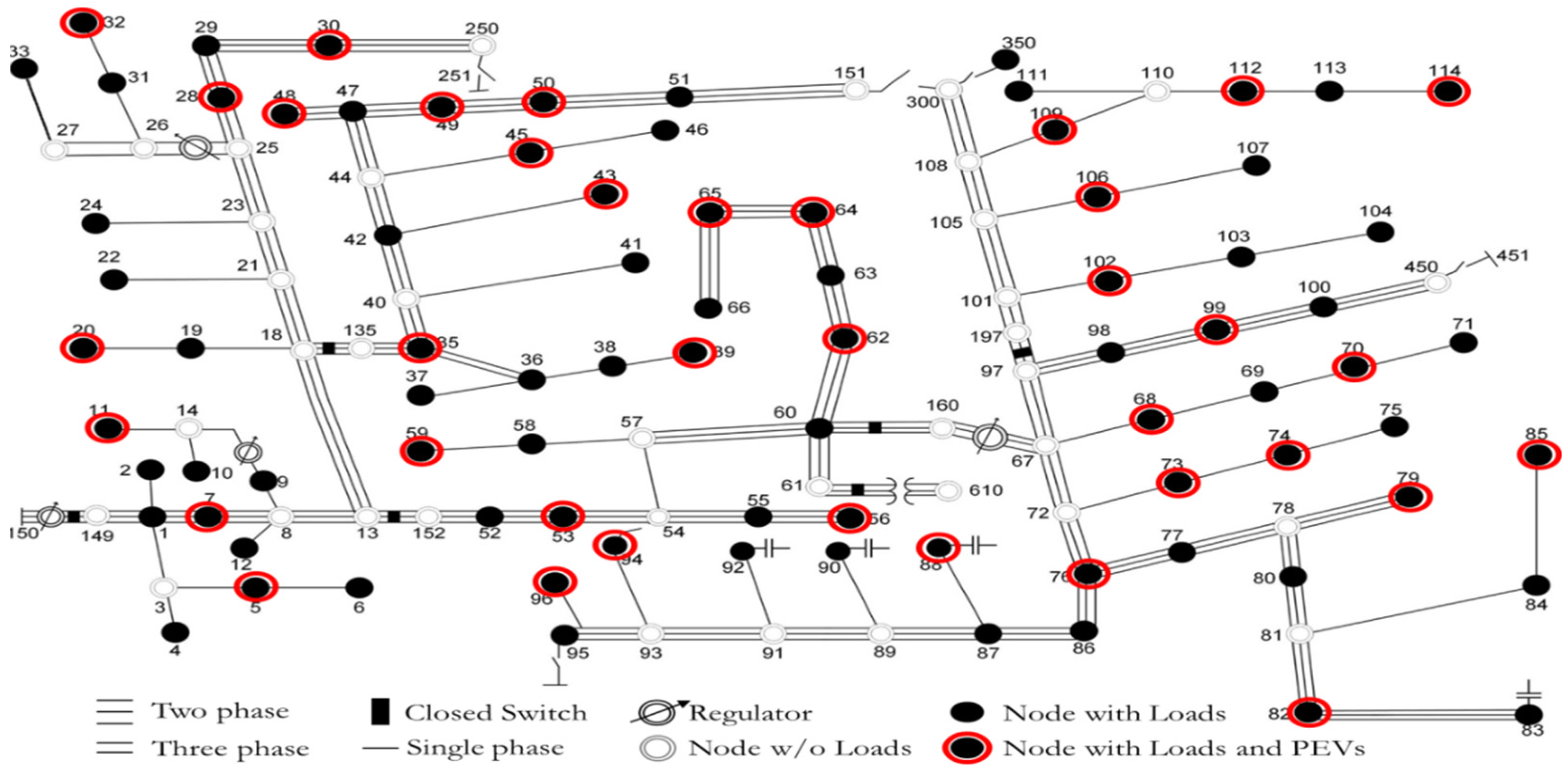
IEEE 123-Node Test Feeder is chosen as a distribution network in OpenDSS (Figure 12);
4-
The distribution network has 123 nodes in which only 85 nodes (black nodes in Figure 12) have loads;
5-
The black nodes in Figure 12 represent the nodes in which homes with only baseloads are supplied, while the black nodes with red circles represent the nodes in which homes with baseloads and the optimized elements (PV, EWH, BSS, and 2 EVs) are supplied;
6-
Two different penetration levels (43% and 100%) of nodes with smart homes are considered.
Figure 13, Figure 14, Figure 15 and Figure 16 compare both methods regarding the voltage drops on the IEEE 123 Node Test Feeder. Different penetration levels of smart homes (43% and 100%) at different times (06:00 and 13:00) are studied. In Figure 13, it is obvious that even a penetration level of 43% can increase the voltage drop on the network for M1, while M2 shows better results even for a penetration level of 100%, as in Figure 14. For the case of M1, most of the nodes on the network faced severe voltage drops below the recommended limit (0.95 p.u.), especially for the phase “a” (black curve). It can be concluded that M2 has improved the voltage stability on the network, even with a very high penetration of EVs.
In Figure 15 and Figure 16, different penetration levels are studied at time 13:00 where the power demands using M1 have the lowest negative values (a negative value indicates a reverse power flow from homes to the grid). Results show that a high reverse power flow raises the voltage on the network above the limit (1.05 p.u.) on many nodes, which may put the network at risk. On the other hand, M2 shows better results in which a smaller number of nodes is above the voltage limit, even with a 100% penetration level of EVs.
Figure 17 presents the line losses on the network for both methods. M2 is better at time 06:00 (Figure 17a), in which line losses are reduced by at least 72% (43% penetration level of EVs) and by a maximum of 80.6% (for 100% penetration level of EVs). However, at time 13:00 (Figure 17b), M1 is better since all homes have lower power demands. A 100% penetration level of EVs using M1 (Figure 17b) shows that line losses become higher, which is caused by a reverse power flow that has increased quadratically the losses on the lines.
To conclude the study, Table 4 presents the income and the cost from the viewpoint of the DSO for a penetration level of 43% (43% of nodes supply smart homes with the optimized elements). For M1, the DSO is collecting 5134.9 $/day from the householders. However, there are high losses on the transformers (−449.5 $/day), lines (−807.1 $/day), and the depreciation cost of the transformers (−294,000 $/day), which is considered the main problem of M1. In total, the DSO is losing (−29,121.7 $/day). The case is different for M2, in which the DSO always has positive revenue. M2 without the incentive program (M2woIP) increases the revenue of the DSO (5781.5 $/day), however, the housholders are not satisfied because they pay more than M1 for consuming the same energy. While for M2 with incentive program (M2wIP), householders pay less compared to M1 and M2woIP. Hence, their satisfaction is increased, but the DSO is reducing its income to 4321.4 $/day (instead of 5781.5 $/day) compared to M2woIP, but its revenue is much better than M1. From this place, M2wIP is recommended to be used because it satisfies both end-users and the DSO for its advantages in reducing the techno-economic losses on the network and minimizing the electricity cost of the end-users. Table 5 presents a comparison between M1 and M2 from the viewpoints of the householders and the DSO. In general, M2wIP is better than M1 in many aspects.

5. Conclusions

This paper presents a novel energy-data management algorithm for a smart transformer, in which the main goal is to propose power and energy soft-constraint limits to homes that should be respected. The power and energy demand at homes should follow these limits in order to guarantee that the total load on the transformer does not exceed its constraints. The novelty of the algorithm can be summarized by the following points: (i) It proposes a variable soft-constrained power profile limit for each home; (ii) It classifies and sorts homes according to their average energy demand from the lowest to the highest; (iii) It proposes decentralized demand response and incentive programs for each individual home; (iv) It allows the homes to share unused energy between them. Our method is compared to an existing one in the literature that uses a conventional transformer. Results show that our method satisfies both end-users and the system operator by (i) reducing the techno-economic losses at homes, transformers, and the network; (ii) maximizing the load factor; (iii) minimizing the peak demand by 57.37% and the power congestion on the network; (iv) maintaining the voltage profile within the recommended limits (reduced by 6.43%); (v) minimizing their electricity cost at homes (≈3% lower); (vi) maximizing the profit of the system operator under certain constraints; (vii) reducing the transformer’s Loss of Life and its depreciation cost by 99.976%; (viii) increasing the revenue of the system operator; (ix) guaranteeing better privacy and security of the consumers since the data are manipulated locally without sending it to the system operator. The limitation of this study is that the protection devices (such as circuit breakers, relays, and fuses) on the transformer are absent. The main reason is to show what will be the impact of both methods, M1 and M2, on the transformer and the network without considering these protection devices. That is why M1 has exceeded twice the transformer’s power limit which can reduce drastically its lifetime and may cause explosion. In future works, many factors will be considered, including the existence of protection devices on the transformer and the network. To do so, we have to improve the algorithm, and add new mathematical equations that represent these protection devices. Therefore, the study will be more realistic and we will study the impact on the network and the consumers when the protection devices are activated.

Author Contributions

Writing—original draft preparation, C.Z.E.-B.; writing—review and editing, U.E., K.A., B.B. and M.Z.; supervision, funding acquisition, U.E. All authors have read and agreed to the published version of the manuscript.

Funding

This research received no external funding.

Conflicts of Interest

The authors declare no conflict of interest.

References

  1. Shao, C.; Wang, X.; Shahidehpour, M.; Wang, X.; Wang, B. Partial Decomposition for Distributed Electric Vehicle Charging Control Considering Electric Power Grid Congestion. IEEE Trans. Smart Grid 2017, 8, 75–83. [Google Scholar] [CrossRef]
  2. Xu, Z.; Su, W.; Hu, Z.; Song, Y.; Zhang, H. A Hierarchical Framework for Coordinated Charging of Plug-In Electric Vehicles in China. IEEE Trans. Smart Grid 2016, 7, 428–438. [Google Scholar] [CrossRef]
  3. Morstyn, T.; Hredzak, B.; Agelidis, V.G. Control Strategies for Microgrids with Distributed Energy Storage Systems: An Overview. IEEE Trans. Smart Grid 2016, 9, 3652–3666. [Google Scholar] [CrossRef] [Green Version]
  4. Fotouhi Ghazvini, M.A.; Soares, J.; Abrishambaf, O.; Castro, R.; Vale, Z. Demand response implementation in smart households. Energy Build. 2017, 143, 129–148. [Google Scholar] [CrossRef] [Green Version]
  5. Wu, X.; Hu, X.; Teng, Y.; Qian, S.; Cheng, R. Optimal integration of a hybrid solar-battery power source into smart home nanogrid with plug-in electric vehicle. J. Power Sources 2017, 363, 277–283. [Google Scholar] [CrossRef] [Green Version]
  6. Steen, D.; Tuan, L.A.; Carlson, O. Effects of Network Tariffs on Residential Distribution Systems and Price-Responsive Customers Under Hourly Electricity Pricing. IEEE Trans. Smart Grid 2016, 7, 617–626. [Google Scholar] [CrossRef]
  7. Wu, X.; Hu, X.; Moura, S.; Yin, X.; Pickert, V. Stochastic control of smart home energy management with plug-in electric vehicle battery energy storage and photovoltaic array. J. Power Sources 2016, 333, 203–212. [Google Scholar] [CrossRef] [Green Version]
  8. Vandael, S.; Holvoet, T.; Deconinck, G.; Nakano, H.; Kempton, W. A Scalable Control Approach for Providing Regulation Services with Grid-Integrated Electric Vehicles. In Design and Analysis of Distributed Energy Management Systems; Springer: Berlin/Heidelberg, Germany, 2020; pp. 107–128. [Google Scholar]
  9. Paterakis, N.G.; Erdinç, O.; Bakirtzis, A.G.; Catalão, J.P.S. Optimal Household Appliances Scheduling Under Day-Ahead Pricing and Load-Shaping Demand Response Strategies. IEEE Trans. Ind. Inf. 2015, 11, 1509–1519. [Google Scholar] [CrossRef]
  10. Melhem, F.Y.; Grunder, O.; Hammoudan, Z.; Moubayed, N. Optimization and Energy Management in Smart Home Considering Photovoltaic, Wind, and Battery Storage System With Integration of Electric Vehicles. Can. J. Electr. Comput. Eng. 2017, 40, 128–138. [Google Scholar] [CrossRef]
  11. Melhem, F.Y.; Grunder, O.; Hammoudan, Z.; Moubayed, N. Thermal and Electrical Load Management in Smart Home Based on Demand Response and Renewable Energy Resources. In Proceedings of the Third International Conference on Electrical and Electronic Engineering, Telecommunication Engineering and Mechatronics (EEETEM2017), Faculty of Engineering, Lebanese University, Beirut, Lebanon, 26–28 April 2017; pp. 1–6. [Google Scholar]
  12. Tomić, J.; Kempton, W. Using fleets of electric-drive vehicles for grid support. J. Power Sources 2007, 168, 459–468. [Google Scholar] [CrossRef]
  13. Kempton, W.; Tomić, J. Vehicle-to-grid power implementation: From stabilizing the grid to supporting large-scale renewable energy. J. Power Sources 2005, 144, 280–294. [Google Scholar] [CrossRef]
  14. Kempton, W.; Tomić, J. Vehicle-to-grid power fundamentals: Calculating capacity and net revenue. J. Power Sources 2005, 144, 268–279. [Google Scholar] [CrossRef]
  15. ABB. TXpert The World’s First Digital Distribution Transformer; ABB Inc.: Raleigh, NC, USA, 2017. [Google Scholar]
  16. Seimens. SensformerTM: Born Connected, Introducing the Digital Transformers Family; Seimens: Erlangen, Germany, 2018. [Google Scholar]
  17. Siemens. Transformers Meet Connectivity: Siemens Introduces Sensformer™ at Hannover Messe; Siemens: Munich, Germany, 2018. [Google Scholar]
  18. Helali, H.; Bouallegue, A.; Khedher, A. A review of smart transformer architectures and topologies. In Proceedings of the 2016 17th International Conference on Sciences and Techniques of Automatic Control and Computer Engineering (STA), Sousse, Tunisia, 19–21 December 2016; pp. 449–454. [Google Scholar]
  19. Chen, Q.; Liu, N.; Hu, C.; Wang, L.; Zhang, J. Autonomous Energy Management Strategy for Solid-State Transformer to Integrate PV-Assisted EV Charging Station Participating in Ancillary Service. IEEE Trans. Ind. Inf. 2017, 13, 258–269. [Google Scholar] [CrossRef]
  20. Mohamed, A.; Salehi, V.; Ma, T.; Mohammed, O. Real-Time Energy Management Algorithm for Plug-In Hybrid Electric Vehicle Charging Parks Involving Sustainable Energy. IEEE Trans. Sustain. Energy 2014, 5, 577–586. [Google Scholar] [CrossRef]
  21. Eshkevari, A.L.; Mosallanejad, A.; Sepasian, M. In-depth study of the application of solid-state transformer in design of high-power electric vehicle charging stations. In IET Electrical Systems in Transportation; Institution of Engineering and Technology: London, UK, 2020. [Google Scholar]
  22. El-Bayeh, C.Z.; Mougharbel, I.; Asber, D.; Saad, M.; Chandra, A.; Lefebvre, S. Novel Approach for Optimizing the Transformer’s Critical Power Limit. IEEE Access 2018, 6, 55870–55882. [Google Scholar] [CrossRef]
  23. IEEE Guide for Loading Mineral-Oil-Immersed Transformers and Step-Voltage Regulators. IEEE Std. C57.91-2011 (Revision of IEEE Std C57.91-1995) 2012, 1–123. [CrossRef]
  24. Rhodes, J.D. The old, dirty, creaky US electric grid would cost $5 trillion to replace. Where should infrastructure spending go? The Conversation, Academic Rigour, Journalistic Flair, 77 Bloor St. W., Suit 600, Toronto M5S 1M2, Canada, 16 March 2017. Available online: https://theconversation.com/the-old-dirty-creaky-us-electric-grid-would-cost-5-trillion-to-replace-where-should-infrastructure-spending-go-68290 (accessed on 8 January 2018).
Figure 1. Simplified flowchart of the proposed energy-management algorithm on the transformer level.
Energies 13 04984 g001
Figure 2. Required data for the smart transformer.
Energies 13 04984 g002
Figure 3. Buying and selling electricity price using real-time price as in [4].
Energies 13 04984 g003
Figure 4. Power demand profiles for the baseload, method 1 and method 2 at home 4.
Energies 13 04984 g004
Figure 5. Power demand profiles for the baseload, method 1 and method 2 at home 10.
Energies 13 04984 g005
Figure 6. Electricity cost at homes in $/Day.
Energies 13 04984 g006
Figure 7. Total power consumption on the distribution transformer.
Energies 13 04984 g007
Figure 8. Voltage deviation on the distribution transformer.
Energies 13 04984 g008
Figure 9. Total energy losses on the transformer and at homes during a day.
Energies 13 04984 g009
Figure 10. Electricity cost of energy losses on the transformer and at homes during a day.
Energies 13 04984 g010
Figure 11. Maximum and minimum power demand during a day.
Energies 13 04984 g011
Figure 12. Schematic Diagram of IEEE 123 Nodes Test Feeder.
Energies 13 04984 g012
Figure 13. Comparing the voltage drops on all buses for M1 and M2 for a penetration level of 43% at time 06:00. (a) Voltage drops on all buses using M1. (b) Voltage drops on all buses using M2.
Energies 13 04984 g013
Figure 14. Comparing the voltage drops on all buses for M1 and M2 for a penetration level of 100% at time 06:00. (a) Voltage drops on all buses using M1. (b) Voltage drops on all buses using M2.
Energies 13 04984 g014
Figure 15. Comparing the voltage drops on all buses for M1 and M2 for a penetration level of 43% at time 13:00. (a) Voltage drops on all buses using M1. (b) Voltage drops on all buses using M2.
Energies 13 04984 g015
Figure 16. Comparing the voltage drops on all buses for M1 and M2 for a penetration level of 100% at time 13:00. (a) Voltage drops on all buses using M1. (b) Voltage drops on all buses using M2.
Energies 13 04984 g016
Figure 17. Impact of using M1 and M2 on the total line losses and for different penetration levels and hours. (a) Total line losses for different penetration levels at time 06:00. (b) Total line losses for different penetration levels at time 13:00.
Energies 13 04984 g017
Table 1. Our proposed incentive program for both power and energy.
Exceeded Value in % π P (Tariff in $/day) π E (Tariff in $/day)
≤0%−2.9−2
>0%00
Remark: $ is in Canadian Dollar in this paper.
Table 2. Comparative criteria were used to evaluate both method 1 (M1) and method 2 (M2).
ConsiderationPower DemandElectricity CostVoltage DeviationLOL of the DTDT Remaining LifetimeDT Depreciation CostEnergy LossesElectricity Cost of the Energy LossesRevenue of the DSO
Homes
Distribution Transformer
Distribution Network
Table 3. Loss of Life (LOL) per day, remaining lifetime, and benchmark depreciation cost of the transformer.
ConsiderationsUnitBase LoadMethod 1Method 2
LOL per Dayday0.2575001.81
year0.0020.550.00
DT Remaining Lifetimeday29,548.461.004142.96
year80.950.0011.35
Benchmark Depreciation Cost *$/day−0.605999.20.65
Depreciation Cost of the DT$/day0.2060001.45
* The Benchmark Depreciation Cost (BDC) means how much the system operator is losing from the value of its transformers per day. (In this paper, we consider that the cost of the considered DT is 6000 $). A value BDC = 0 means that the transformer is not depreciating, a value greater than zero (BDC = 2) means that the system operator is losing about 2 $/day of the depreciation cost of the transformer due to the peak demand.
Table 4. Total revenue of the DSO for a penetration level of 43%.
DescriptionUnitM1M2woIPM2wIP
Electricity tariff paid by consumers to the DSO$/Day5134.96442.94982.8
Cost of total losses on the lines$/Day−807.1−316.4−316.4
Cost of total losses on the transformers$/Day−449.5−260.3−260.3
Depreciation cost of the transformers (Average cost of the transformer is CAD 6000)$/Day−294,000−71.0−71.0
Upgrading cost of the infrastructure
(≈35% of the actual infrastructure) *
$/Day0−13.7−13.7
Total revenue of the DSO$/Day−290,121.75781.54321.4
* According to [24], 35% additional cost is required to upgrade the existing infrastructure of the Distribution Network (DN). In this table, only 43% of the DN (IEEE 123 node test feeder) is upgraded, since only 43% of the total network is used to integrate EVs.
Table 5. Summary of the comparison between methods 1 (M1) and method 2 with incentive program (M2wIP).
LevelDescriptionM1M2wIP
HomeMinimize the electricity cost34
(≈2.96% lower)
Consumers are satisfied34
Low risk of damaging equipment24
DT and DN constraints are considered14
Reduce the voltage drop24
Respect the soft-constraint power limit14
Distribution TransformerRespect the critical power limit14
Reduce the Loss of Life14
Increase the remaining lifetime14
Reduce the depreciation cost14
(reduced by 42%)
Reduce the energy losses and their associated cost14
(reduced by 42%)
Reduce the voltage drop14
Reduce the risk of damage and explosion, which may lead to environmental disasters14
Reduce installation cost41
(higher by 35%)
Reduce the simulation time *34
(36.4% lower)
Distribution SystemRespect the voltage limits (e.g., between 0.95 and 1.05)24
Reduce the energy losses and their associated cost14
(reduced by 80%)
Increase the total revenue of the DSO14
Reduce the investment cost42
Likert scale: “1” Strongly disagree, “2” disagree, “3” agree, “4” Strongly agree. * The simulation was performed using MATLAB and OpenDSS. The used mathematical programming is Mixed-Integer Nonlinear Programming (MINLP), using the function fmincon in MATLAB (MathWorks, Natick, MA, USA).

