Spatial Effects and Nonlinear Analysis of Energy Consumption, Financial Development, and Economic Growth in China

Abstract

Energy consumption is of great significance to the sustainable development of the economy. Due to the spatial heterogeneity of low-carbon growth in regional economies, the relationship between energy consumption and economic growth is complicated. However, a few researches have been published about spatial spillover effects and non-linearity of energy consumption and financial development on regional economic growth in China. Based on the panel data of 30 provinces in China from 2007 to 2017, this paper analyzes the spatial spillover effects and threshold effects of energy consumption and financial development on regional economic growth by using spatial and nonlinear econometric methods. The main conclusions are as follows. Spatial econometric methods show that financial development and energy consumption are two factors of production input to promote China’s economic growth. Meanwhile, energy consumption and financial development have spillover effects on regional economic growth. Additionally, the nonlinear econometric method finds that with increasing financial development, the impact of energy consumption on economic growth is segmented. Therefore, relevant policies should be implemented to enhance the role of finance in energy consumption to promote low-carbon growth of China’s economy.

1. Introduction

Energy consumption is vitally important to the national economy, people’s livelihoods and national security, as well as to the prosperity of a country and the well-being of its people. Currently, China has become the largest energy consumer in the world [1]. At the beginning of the founding of the People’s Republic of China, China’s energy base was weak. In the past 70 years, China’s energy industry has undergone tremendous changes. With the rapid development of China’s economy, the overall energy consumption is growing rapidly. During the 11th Five-year Plan period (2006–2010), the target for energy consumption per unit of GDP in 2010 was about 20% lower than that in 2005. During the 12th Five-year Plan period (2011–2015), the target for energy consumption per unit of GDP in 2015 was over 16% lower than that in 2010. During the 13th Five-year Plan period (2016–2020), the target for energy consumption per unit of GDP in 2020 is 15% lower than that in 2015, and energy consumption per unit of GDP was actually reduced by 11.4% in 2018. Since the 18th National Congress of the Communist Party of China (CPC), the Chinese government has put forward the strategic idea of “energy revolution”.

In this economic situation, having a solid financial system is essential to provide effective financing, market liquidity and risk management [2]. Facing the complex and grim international environment and arduous tasks of reform, development and stability, financial development is crucial to China’s sustainable economic development. According to National Bureau of Statistics of China [3], savings deposit in Renminbi (RMB) and foreign currencies in all items of financial institutions totaled 28.7 trillion dollars at the end of 2019, an increase of 2.3 trillion dollars compared with that at the beginning of the year. Specifically, the savings deposit in RMB stood at 28.0 trillion dollars, an increase of 2.2 trillion dollars. Loans in RMB and foreign currencies in all items of financial institutions reached 23.0 trillion dollars, an increase of 2.4 trillion dollars. Of this total, loans in RMB were 22.2 trillion dollars, an increase of 2.4 trillion dollars. Reasonable credit supply creates a favorable financial environment for high-quality economic development. In an economic environment that highly encourages energy development, the role of financial development is considerably important.

A multiplicity of economic growth literature has established that financial development and energy consumption are crucial elements to the development of social productivity [4,5,6,7]. In the course of China’s energy revolution strategy, exploring the influence of energy consumption and financial development on economic growth is conducive to optimizing the energy ecosystem and realizing the coordinated development of multi-agent economy. Figure 1 shows energy consumption (EC, measured by total energy consumption), financial development (FD, measured by credit funds of financial institutions) and Gross Domestic Product (GDP) of China from 2007 to 2019. As can be seen from Figure 1, GDP has maintained steady growth. The change of EC is similar to GDP. From a national perspective, FD basically maintained steady and rapid growth from 2007 to 2019. By comparing the trends of economic growth, financial development, and energy consumption, this paper also finds that there is a certain correlation and similarity. Therefore, it is practically significant to analyze the effect of financial development and energy consumption on economic growth.

Most researchers focus on energy consumption surge. However, a few researchers have been published about the spatial spillover effects and non-linearity of energy consumption and financial development on regional economic growth in China. Then, facing the spatial heterogeneity of China’s regional economic distribution, does China’s regional economy have spatial spillover effect? Does energy consumption restrain or promote China’s regional economic growth? With the Chinese government’s attention to low-carbon economy, how can energy consumption further affect China’s economic sustainable development through financial means? The study of these issues is not only conducive to the enrichment of low-carbon economic theory, but also contributes to the sustainable development of China’s economy and the realization of high-quality economic development. Therefore, the control of energy consumption is the key to achieving economic sustainability and sustainable utilization of resources.

2. Literature Review

Currently, there are many disputes in the research of energy consumption, financial development, and economic growth. We examine the existing literature from three perspectives. Summary of the existing empirical studies is shown in Appendix A with

Table A1. Summary of the existing empirical studies.

Authors	Countries	Periods	Methodologies	Main Conclusion
Energy Consumption and Economic Growth
Acheampong (2018)	116 countries	1990–2014	PVAR and S-GMM	EC→GDP
Wang et al. (2015)	China	1990–2012	Cointegration and granger causality tests	EC↔GDP
Liu and Hao (2018)	69 countries of the Belt and Road	1970–2013	VECM, FMOLS and DOLS	Energy use ↔ GDP per capita (in the long run)
Shahbaz et al. (2018)	10 countries	1960Q1–2015Q4	Quantile-on-quantile approach	GDP→EC (with variations across each country)
Aydin and Esen. (2017)	12 countries	1991–2013	Dynamic panel threshold analysis	EC $\stackrel{-}{\to }$ GDP (energy intensity ≥ 0.44%), EC $\stackrel{+}{\to }$GDP (energy intensity ≤ 0.44%)
Hao et. al.(2018)	China	1995–2010	VECM, FMOLS, IRF	Rural GDP ↔ rural EC (in the short run)
Financial Development and Economic Growth
Yang (2019)	49 mid-income countries	1960–2016	Granger causality	FD$\stackrel{+}{\to }$GDP
Sassi and Gasmi (2014)	27 European countries	1995–2012	OLS, GMM panel	FD$\stackrel{-}{\to }$GDP
Law and Singh (2014)	87 countries	1980–2010	Dynamic panel threshold	There is a threshold effect in the finance–growth relationship
Yang(2014)	China	1987–2009	Panel threshold model	Threshold effect and diminishing marginal efficiency
Liu and Zhang (2018)	China	1996–2013	Panel quantile regression	FD→GDP(different with different regions and stages)
Energy Consumption, Financial Development, and Economic Growth
Eren et al. (2019)	India	1971–2015	Cointegration test, DOLS and granger causality test	REC and GDP are FD driven in the long run. REC↔GDP
Ouyang and Li (2018)	China	1996Q1–2015Q4	GMM panel VAR and PCA	FD$\stackrel{-}{\to }$GDP, EC→GDP, FD→EC(↓)
Shahbaz et al. (2017)	India	1960Q1–2015Q4	A nonlinear and asymmetric analysis	(only negative shocks) FD→GDP, (only negative shocks)EC→GDP
Komal and Abbas (2015)	Pakistan	1972–2012	S-GMM	EC→GDP, FD$\stackrel{\mathrm{GDP}}{\to }$EC
Khan et al. (2019)	193 countries	1990–2017	3SLS, dynamic model 2-step GMM, S-GMM	EC→FD(↓)

.

2.1. Energy Consumption and Economic Growth

With the rapid development of the economy, it is particularly critical to study energy consumption for solving environmental problems and realizing sustainable development. The energy–growth nexus can be described mainly from three aspects. Firstly, the energy–growth nexus is causality running bi-directionally [9,10,11]. For example, based on 69 countries of the Belt and Road for the period of 1970–2013, Liu and Hao [10] employed vector error correction model (VECM), granger causality, fully modified ordinary least squares (FMOLS), and dynamic OLS (DOLS) approaches and considered that energy use and GDP per capita had a bi-directional causal relationship in the long run. Hao et al. [11] introduced VECM, FMOLS, impulse response function (IRF), and variance analysis and drew a conclusion that Chinese rural GDP and energy consumption (EC) had bi-directional causal relationship in the short run. Secondly, energy consumption is critical to economic growth [12]. Gozgor et al. [13] decomposed energy consumption into renewable energy consumption (REC) and non-renewable energy consumption (NREC), and investigated 29 OECD countries for the period 1990–2013. They theoretically and empirically explained the contribution of REC and NREC to GDP. Contrastively, some literature suggested that economic growth had a positive impact on energy consumption [14], which varied in different periods [15] and different countries [16]. Shahbaz et al. [16] used a quantile-on-quantile approach to study the data of ten energy-consuming countries from 1960Q1 to 2015Q4, and explained that economic growth had a positive effect on energy consumption with considerable variations across economic states in each country. However, other literature has shown non-linear effects on energy consumption and economic growth. Aydin and Esen [17] applied dynamic panel threshold analysis and confirmed when the energy intensity was greater than or equal to 0.44%, EC had a negative impact on economic growth. While the energy intensity was less than 0.44%, EC had a positive impact on economic growth. Bekun et al. [18] believed an inverted U-shaped pattern between energy use and economic growth in South Africa from 1960 to 2016. The findings indicated that the intensity of energy consumption was relatively low at a higher level of economic development. The lack of consensus and the limitations in these papers may be due to the heterogeneity of countries, different stages of economic growth and differences in methodologies used.

2.2. Financial Development and Economic Growth

One of the core problems of financial development theory is the nexus between financial development and economic growth. Since King and Levine [19], the multiformity of the literature on financial development and economic growth has mushroomed. The previous literature can be summarized as three main aspects. Firstly, financial development has a positive impact on economic growth [19,20]. Based on a Schumpeterian growth model, Diallo and Al-Titi [21] concluded that financial development had an important impact on local economic growth. Using the data from the Beijing–Tianjin–Hebei region of China, Wang et al. [22] had the same standpoint as Diallo and Al-Titi [21]. Secondly, financial development has a negative impact on economic growth [23,24]. Using data of 27 European countries over the period 1995–2012, Sassi and Gasmi [23] employed the negative effect of financial development on economic growth and the heterogeneity of financial development. However, other studies have demonstrated that non-linearity exists between financial development and economic growth [25,26,27,28,29,30]. As an empirical example, Liu and Zhang [25] explored the endogenous mechanism of financial structure and economic growth based on the data of 29 provinces in China from 1996 to 2013, and found that the influence of financial structure on economic growth was inverse-U shaped. Law and Singh [26] used data from 87 countries between 1980 and 2010 to provide new evidence of a non-linear relationship between financial development and economic growth. They studied stylized facts that there were threshold effects between financial development and economic growth and highlighted that too much finance harmed economic growth. Virtually, the effects of China’s financial development on economic growth were also manifested by the non-linear characteristics of threshold effects and diminishing marginal efficiency, and the form of the nonlinear relationship was different in different provinces of China [27,28,29]. Huang and Lin [30] employed a novel threshold regression with the instrumental variables approach to deal with the endogenous problems of financial development and economic growth. From the above theoretical and empirical analysis, these literature have not reached a consensus.

2.3. Energy Consumption, Financial Development and Economic Growth

Overall, a review of the existing literature indicates that there is little research on the nexus between energy consumption, financial development and economic growth. The results can be roughly summarized in two aspects. Firstly, energy consumption and financial development have a direct impact on economic growth, but the impact results are inconsistent. Some studies considered that a bi-directional causal relationship exists among them. Shahbaz et al. [5] introduced the Autoregressive Distributed Lag (ARDL) bounds, structural break test, and drew the conclusions that financial development and energy consumption had a positive significantly impact on economic growth in the case of China over the period of 1971–2011. Moreover, there was a bi-directional causal nexus between financial development and energy consumption. Eren et al. [2] used the data from India for the period of 1971–2015 and employed cointegration test, DOLS, and granger causality test under a vector error correction model. They found that REC and economic growth were financial development driven in the long run. Furthermore, REC has a bi-directional causal relationship with economic growth. Other studies considered that there was a unidirectional effect among them. Using data of China over the period 1996Q1 to 2015Q4, Ouyang and Li [24] introduced Generalized Method of Moments (GMM) panel Vector Autoregressive (VAR) approach and principal component analysis (PCA) to explain that financial development had a significant negative impact on economic growth. Except in the western region, energy consumption had a positive impact on economic growth. Moreover, financial development can significantly reduce energy consumption in all regions. Al-Mulali and Sab [31] used the panel data of 19 countries over the period of 1980–2008 by Pedroni (Engle–Granger based) cointegration tests and panel granger causality found that energy consumption enables these countries to achieve high economic and financial development. What is more, compared with the aforementioned approaches, Khan et al. [7] applied seemingly unrelated regression (SUR), three stage least squares regression (3SLS), and two-step system generalized method of moments approach (2S-GMM) and found similar conclusions. Secondly, economic growth acts as an intermediary, driving financial development to influence energy consumption. For instance, Komal and Abbas [32] found that energy consumption had a significantly positive impact on economic growth. Simultaneously, based on the S-GMM method, they also found that financial development has a positive and significant impact on energy consumption through the intermediary role of economic growth. Therefore, the nexus among energy consumption, financial development and economic growth is considerably complex. More importantly, non-linearity has not been taken into account.

2.4. Summary of the Aforementioned Literature

The nexus between resource conservation and economic sustainability is realized through energy consumption and financial development [33]. Exploring the nature of the links amongs energy consumption, financial development, and economic growth is of great significance for central policy makers to formulate optimal energy and economic policies. By summarizing the aforementioned literature, this paper makes three primary contributions to the existing literature.

Firstly, although the research on financial development, energy consumption and economic growth has received great attention both theoretically and empirically, there is still a significant gap in the conclusion of the available literature. For instance, Liu and Hao [10] and Hao et al. [11] drew a conclusion that GDP and EC had a bi-directional causal relationship, while Shahbaz et al. [16] explained that economic growth has a significantly positive effect on energy consumption. Diallo and Al-Titi [21] and Wang et al. [22] concluded that financial development had an important impact on economic growth, while Sassi and Gasmi [23], Ouyang and Li [24], and Liu and Zhang [25] found a negative influence of financial development on economic growth. Additionally, Khan et al. [7] and Al-Mulali and Sab [31] found that energy consumption enables these countries to achieve high economic and financial development. This paper empirically studies the impact of energy consumption and financial development on economic growth based on the data of 30 provinces in China from 2007 to 2017.

Secondly, the financial effect of energy consumption on economic growth is spatially heterogeneous, and this phenomenon is related to different periods and different regions [15,16,25]. Yuan et al. [15] used grey incidence analysis to study Chinese economic growth and energy consumption from 1985 to 2007. Empirical results showed that the relations between Chinese economic growth and energy consumption in different periods are not the same. Shahbaz et al. [16] employed the data of economic growth and energy consumption in ten energy-consuming countries from 1960Q1 to 2015Q4, and explained that economic growth has a positive effect on energy consumption with considerable variations across economic states in each country. Simultaneously, based on the data of 29 provinces in China from 1996 to 2013, Liu and Zhang [25] found that the influence of financial structure on economic growth in different regions is different, and at different stages of economic development, the influence of financial structure on economic growth is anti-U-shaped. However, the available literature rarely discusses how the financial effects of energy consumption affect economic growth. Eren et al. [2] found that economic growth was promoted by financial development driven REC. Shahbaz et al. [6] found that only negative shocks to energy consumption and financial development would have an impact on economic growth. To sum up, the study of the financial effects of energy consumption on economic growth is complex, and many studies have the drawback of simplification. Therefore, this paper studies the spatial complexity from two aspects: direct path and indirect path (financial effects).

Thirdly, the spatial effects and nonlinearity of financial development and energy consumption on economic growth are seldom considered in previous studies. Traditional econometric methods, such as VECM and FMOLS [10,11], DOLS [2,10], IRF [11], GMM and VAR [24], SUR and 3SLS [7], and S-GMM [7,32], ignore the spatial effect. A spatial econometric model is established from a macro perspective to empirically analyze the spillover effect in this paper. Furthermore, Aydin and Esen [17] and Bekun et al. [18] only have shown non-linear effects on energy consumption and economic growth, while Law and Singh [27], Yang [28], Chen et al. [29], and Huang and Lin [30] only have demonstrated that non-linearity exists between financial development and economic growth. The non-linearity of energy consumption and financial development on economic growth is rarely studied. The threshold model is one of the most widely used nonlinear models [1]. The panel threshold model can accurately estimate the threshold value and avoid the bias caused by subjective judgment [34]. Therefore, this paper introduces the panel threshold models to analyze the non-linearity.

The rest of this paper is arranged as follows. Section 3 describes data and variables selection and introduces spatial econometric methods and non-linear econometric methods. Section 4 empirically analyzes spillover effects and non-linearity. Finally, the conclusions and policy propositions are drawn in Section 5.

3. Methodology

3.1. Variables and Data

The data are from the panel data of 30 provinces in China from 2007 to 2017. Taiwan, Hong Kong, Macao, and Tibet are not taken into account due to the lack of energy consumption statistics. The data of financial development come from the China Statistical Yearbook published by the China National Bureau of Statistics, Statistical Bulletin of National Economic and Social Development of each province of China, Regional Financial Operation Report of the People’s Bank of China. Energy consumption data are taken from China Energy Statistical Yearbook (2007–2017). Economic growth data, provincial capital investment data, labor input data, the level of openness data, and the fiscal expenditure data are taken from China Statistical Yearbook (2007–2017).

(1) Economic Growth

Economic growth is the explained variable. GDP denotes gross domestic product. In empirical analysis, researchers often use two methods to measure economic growth. One is to take the GDP of each region and convert it into the real GDP expressed in terms of the base year constant price by the GDP indicator. The other is that GDP per capita can only be used to approximate the level of regional economic development. Most studies believe that the most direct way to measure regional economic growth properly is to measure real GDP in constant price. Therefore, on the basis of 2007, the real GDP expressed in constant prices is used to reflect regional economic growth.

(2) Financial Development

Banks play an important role in China’s financial development and economic growth, because banks provide most of the financial resources in China’s financial system. In the previous literature, bank credit is considered an important financial service to promote economic growth. Therefore, bank credit is often used as an important financial development indicator. This indicator can measure the important role of financial credit in economic growth and is the main source of enterprise financing. Considering the characteristics of China’s financial market and the availability of data, this paper uses the balance of credit funds of financial institutions to reflect the development of regional credit.

(3) Energy Consumption

Energy is an important factor affecting economic growth. In this paper, energy consumption is included in the economic growth model [11]. Total energy consumption refers to the total consumption of energy of various kinds by economic production departments and households in a certain period. Therefore, this paper uses total energy consumption to measure energy consumption.

Through the above theoretical analysis, reasonable financial development can change the impact of energy consumption on economic growth. Therefore, this paper introduces the intersection of financial development and energy consumption (EC*FD) to explore the impact of the current energy policies of China on economic growth by changing the financial effects.

According to the availability of economic theory and data, the control variables of this paper are as follows. Provincial capital investment (K) is expressed by total investment in fixed assets in the whole country. Labor input (L) is expressed by number of employed persons in urban units. The level of openness (Open) is expressed by total value of imports and exports of goods by region where the business unit is located. The fiscal expenditure (Fis) is expressed by local governments general budgetary expenditure. We take logarithms of all variables to reduce heteroscedasticity.

Table A2. Statistical description of variables.

Variables	Mean	Std. Dev.	Min	Max
Economic Growth(lnGDP)	9.343	0.920	6.681	11.227
Total Energy Consumption(lnEC)	9.319	0.686	6.963	10.569
Financial development (lnFD)	9.592	0.964	6.581	11.745
The Intersection (lnEC*lnFD)	89.856	14.126	49.530	121.966
Capital Investment of Provinces(lnK)	9.098	0.915	6.179	10.919
Labor Input(lnL)	5.995	0.766	3.815	7.588
The level of Openness (lnOpen)	8.897	2.220	3.840	14.311
Fiscal expenditure (lnFis)	7.922	0.731	5.488	9.618

Data source: China Statistical Yearbook. Std. Dev. is the abbreviation of standard deviation.

in Appendix A shows the statistical description of all variables used in this paper. All variables have good statistical characteristics.

3.2. Spatial Econometric Methods

Based on the Cobb–Douglas production function and taking energy consumption and financial development as input factors, this paper establishes a logarithmic production function model to analyze the impact of energy consumption and financial development and their interaction on economic growth.

$$\ln GD{P}_{it}={\beta }_1\ln E{C}_{it}+{\beta }_2\ln F{D}_{it}+{\beta }_3\ln (E{C}_{it})*\ln (F{D}_{it})+\gamma \ln X_{it}+{\epsilon }_{it}$$

(1)

where the interaction term, $\ln \left(\mathrm{EC}\right)*\ln (\mathrm{FD})$, denotes the impact of the integration of total energy consumption and financial development on economic growth. $X_{it}$ denotes other control variables affecting economic growth, ${\beta }_1,{\beta }_2,{\beta }_3,\gamma$ denotes regression coefficient of each variable respectively, ${\epsilon }_{it}$ denotes error term, $i$ involves 30 provinces in China and $t$ ranges from 2007 to 2017.

In addition to energy consumption and financial development, regional economic growth is affected by a series of other factors, such as ${\mathrm{K}}_{\mathrm{it}}$, $L_{it}$, $Ope{n}_{\mathrm{it}}$, and $\mathrm{F}i{\mathrm{s}}_{\mathrm{it}}$. By incorporating these control variables into the equation, Equation (1) can be transformed into:

$$\begin{array}{l}\ln GD{P}_{it}={\beta }_1\ln E{C}_{it}+{\beta }_2\ln F{D}_{it}+{\beta }_3\ln (E{C}_{it})*\ln (F{D}_{it})+{\gamma }_1\ln {\mathrm{K}}_{\mathrm{it}}\\ +{\gamma }_2\ln L_{it}+{\gamma }_3\ln \mathrm{O}pe{n}_{\mathrm{it}}+{\gamma }_4\ln {\mathrm{Fis}}_{\mathrm{it}}+{\epsilon }_{it}\end{array}$$

(2)

Equation (2) is an ordinary panel model. If we only consider the spatial effect of GDP, we establish the spatial autoregressive model (SAR), spatial error model (SEM), and spatial durbin model (SDM) [35]. SAR is a spatial econometric model with spatial lag added to the explained variables. SEM is a spatial econometric model that introduces error terms into spatial autocorrelation. SDM is a spatial econometric model that considers both space lag and space error terms. Equations (3)–(5) are SAR, SEM, and SDM, respectively.

$$\begin{array}{l}\ln GD{P}_{it}=\rho W\ln GD{P}_{it}+{\beta }_1\ln E{C}_{it}+{\beta }_2\ln F{D}_{it}+{\beta }_3\ln (E{C}_{it})*\ln (F{D}_{it})+{\gamma }_1\ln {\mathrm{K}}_{\mathrm{it}}\\ +{\gamma }_2\ln L_{it}+{\gamma }_3\ln \mathrm{O}pe{n}_{\mathrm{it}}+{\gamma }_4\ln {\mathrm{Fis}}_{\mathrm{it}}+{\epsilon }_{it}\end{array}$$

(3)

$$\begin{array}{l}\ln GD{P}_{it}={\beta }_1\ln E{C}_{it}+{\beta }_2\ln F{D}_{it}+{\beta }_3\ln (E{C}_{it})*\ln (F{D}_{it})+{\gamma }_1\ln {\mathrm{K}}_{\mathrm{it}}\\ +{\gamma }_2\ln L_{it}+{\gamma }_3\ln \mathrm{O}pe{n}_{\mathrm{it}}+{\gamma }_4\ln {\mathrm{Fis}}_{\mathrm{it}}+\lambda W{\epsilon }_{it}+{\mu }_{it}\end{array}$$

(4)

$$\begin{array}{l}\ln GD{P}_{it}=\rho W\ln GD{P}_{it}+{\beta }_1\ln E{C}_{it}+{\beta }_2\ln F{D}_{it}+{\beta }_3\ln (E{C}_{it})*\ln (F{D}_{it})+{\gamma }_1\ln {\mathrm{K}}_{\mathrm{it}}\\ +{\gamma }_2\ln L_{it}+{\gamma }_3\ln \mathrm{O}pe{n}_{\mathrm{it}}+{\gamma }_4\ln {\mathrm{Fis}}_{\mathrm{it}}+\lambda W{\epsilon }_{it}+{\mu }_{it}\end{array}$$

(5)

where $\rho$ and $\lambda$ respectively denote the regression coefficients of spatial lag and spatial error, and reflect the spillover effect of gross domestic product. $W$ is a spatial weight matrix, which represents the spatial relationships among the various regions.

3.3. Selection of Spatial Weight Matrix

In order to establish a spatial econometric model, this paper firstly defines the space distance. The distance here is generalized, and can be geographic distance, or can be another economic sense of distance. The spatial data of n regions are expressed as ${\left\{x_i\right\}}_{i=1}^n$, $i$ denotes the region $i$. $w_{ij}$ denotes the spatial distance between the region $i$ and the region $j$, then the spatial weight matrix can be defined as

$$W=\left[\begin{array}{ccc}{w}_{11}& \cdots & w_{1n}\\ ⋮& \ddots & ⋮\\ w_{n1}& \cdots & w_{nn}\end{array}\right]$$

(6)

where $w_{ii}=0(i=1,\cdots ,n)$. Because the distance from region $i$ to region $j$ is the same as that from region $j$ to region $i$, that is $w_{ij}=w_{ji}$, the spatial weight matrix $W$ is a symmetric matrix. The most commonly used spatial weight matrix is adjacency matrix (W). Therefore, this paper selects W. Specifically, if regions $i$ and $j$ have common boundary, the weight is 1, otherwise it is 0.

3.4. Nonlinear Econometric Methods

Energy consumption and financial development may have a nonlinear relationship with economic growth. Therefore, the panel threshold model is introduced to analyze the nonlinearity [34]. Economic growth is the explained variable, energy consumption and financial development are the core explanatory variables, and q_it is the threshold variable. In this paper, EC and FD are used as q_it, respectively. The threshold model (single threshold) is as follows,

$$\ln GD{P}_{it}={\alpha }_0+{\alpha }_1\ln F{D}_{it}•I(q_{it}\le \theta )+{\alpha }_2\ln F{D}_{it}•I(q_{it}\ge \theta )+{\alpha }_3\ln X_{it}+{\epsilon }_{it}$$

(7)

$$\ln GD{P}_{it}={\alpha }_0+{\alpha }_1\ln E{C}_{it}•I(q_{it}\le \theta )+{\alpha }_2\ln E{C}_{it}•I(q_{it}\ge \theta )+{\alpha }_3\ln X_{it}+{\epsilon }_{it}$$

(8)

where $I(•)$ is the indicative function. θ represents threshold value. ${\epsilon }_{it}$ represents the residual term, and ${\epsilon }_{it}~i.i.dN(0,{\sigma }^2)$. The multi-threshold model (double threshold as an example) is shown below. If the two threshold values are ${\theta }_1<{\theta }_2$, then

$$\begin{array}{l}\ln GD{P}_{it}={\alpha }_0+{\alpha }_1\ln F{D}_{it}•I(q_{it}\le {\theta }_1)+{\alpha }_2\ln F{D}_{it}•I({\theta }_1<q_{it}\le {\theta }_2)\\ +{\alpha }_3\ln F{D}_{it}•I(q_{it}>{\theta }_2)+{\alpha }_4\ln X_{it}+{\epsilon }_{it}\end{array}$$

(9)

$$\begin{array}{l}\ln GD{P}_{it}={\alpha }_0+{\alpha }_1\ln E{C}_{it}•I(q_{it}\le {\theta }_1)+{\alpha }_2\ln E{C}_{it}•I({\theta }_1<q_{it}\le {\theta }_2)\\ +{\alpha }_3\ln E{C}_{it}•I(q_{it}>{\theta }_2)+{\alpha }_4\ln X_{it}+{\epsilon }_{it}\end{array}$$

(10)

4. Results and Discussion

A lot of economic data involve certain spatial region information. In fact, the economy of each province has a close connection, and the closer the province is, the more frequent the economic interaction. According to Tobler’s [36] first law of geography, all things are related to other things, but those that are closer are more related than those that are farther away. According to LeSage and Pace [34], the influence of various factors on economic growth can be further decomposed into the direct effect and spatial spillover effect (i.e., indirect effect). The impact of a certain factor change in a province on the regional economic growth is a direct effect. The impact of a certain factor change in a province on the economic growth of other regions is a spatial spillover effect. When there is spatial spillover effect, the change of energy consumption, financial development, and the interaction term will not only cause the change of economic growth of the province, but also affect the economic growth of neighboring provinces [1,34].

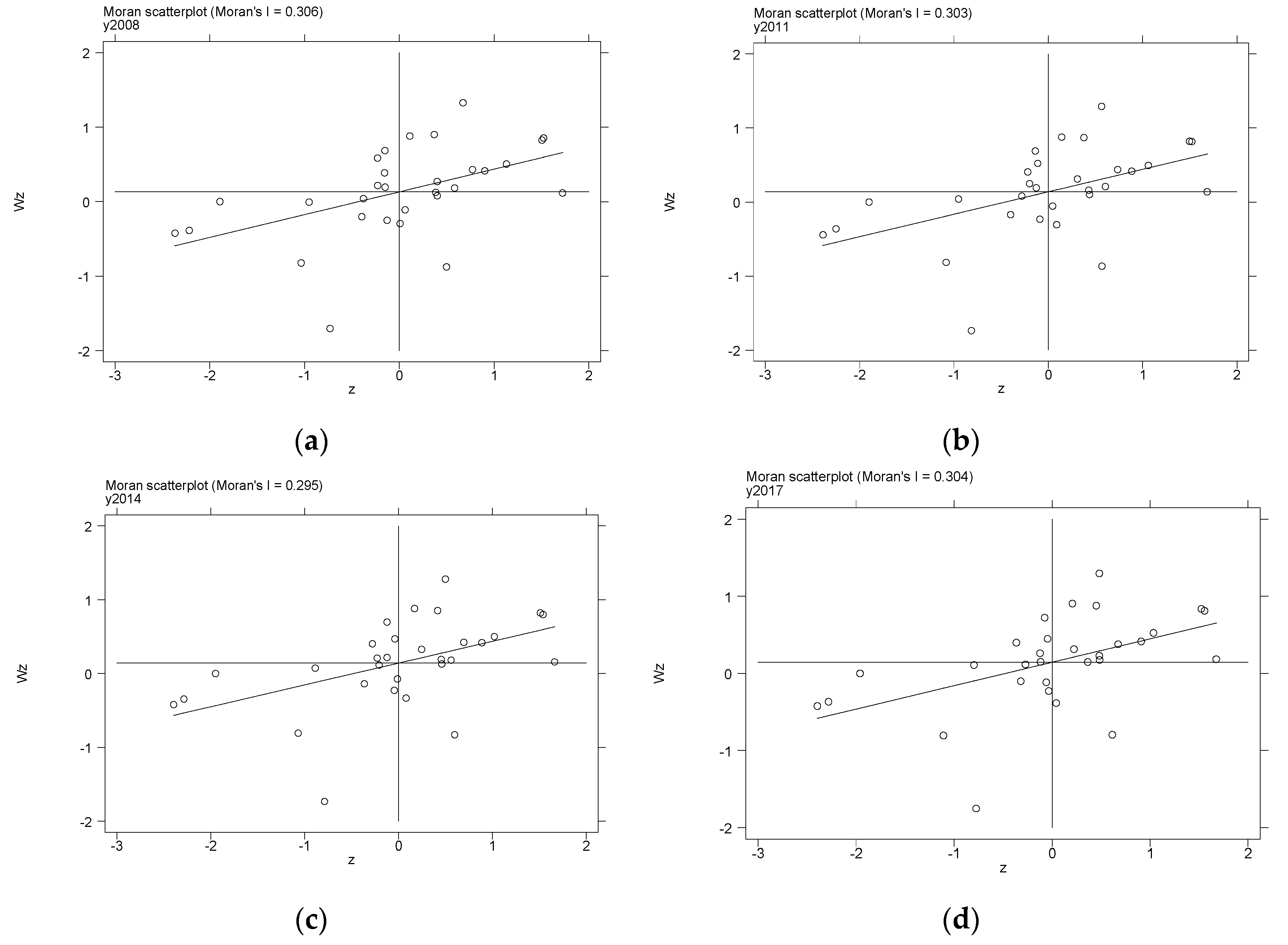
4.1. Spatial Correlation Tests

Before the analysis of the spatial spillover effect, it is necessary to test the spatial autocorrelation characteristics of economic growth. If there is a spatial autocorrelation of economic growth, then the value of economic growth in adjacent regions is similar. If the high-high and low-low values of regional economic growth are clustered together, the regional economic growth has positive autocorrelation. If the high-low values of regional economic growth are clustered together, the regional economic growth has negative autocorrelation. If the high and low values of regional economic growth are randomly distributed, there is no spatial autocorrelation between regional economic growth. This paper adopts the most popular metric spatial autocorrelation method—Moran’s I [37]. The test results of economic growth are shown in Appendix A in

Table A3. lnGDP Moran’s I in China from 2007 to 2017.

Year	2007	2008	2009	2010	2011	2012	2013	2014	2015	2016	2017
lnGDP	0.315	0.316	0.315	0.318	0.314	0.308	0.307	0.306	0.306	0.309	0.314
Z-value	2.918	2.926	2.917	2.939	2.908	2.867	2.855	2.848	2.851	2.875	2.919
p-value	0.002	0.002	0.002	0.002	0.002	0.002	0.002	0.002	0.002	0.002	0.002

. From Table A3, we can see that the Moran’s I of economic growth in 2007–2017 is concentrated in 0.306–0.318, and passed the significance level test of 1%. It shows that the economic growth of 30 provinces in China is not randomly distributed in space, but has a positive autocorrelation in space and presents a strong spatial agglomeration in geographical space.

The Moran’s I scatter plot of regional economic growth is further developed to illustrate the spatial autocorrelation characteristics of economic growth. This paper selects data from 2008, 2011, 2014, and 2017, which correspond to Figure 2a–d respectively. Moran’I scatter plots are divided into four quadrants. Positive spatial correlations are distributed in the first and third quadrants, while negative spatial correlations are distributed in the second and fourth quadrants. As can be seen from the figure, provinces in the first and third quadrants account for more than 67%. This indicates that China’s regional economic growth shows the characteristics of high-high value agglomeration and low-low value agglomeration. Due to China’s vast territory, there are huge differences in economic development and resource conditions between regions, as well as in regional economic growth. According to the change of the time series of the Moran’s I scatter plot, it can be seen that the number of provinces distributed in each quadrant is basically unchanged, indicating that the economic growth in China shows spatial dependence.

4.2. Analysis of Spatial Econometric Models

Because of the significant spatial correlation of regional economic growth in China, the spatial panel model is introduced in this paper. According to the model discriminant criteria of Anselin et al. [38], the spatial econometric models are tested by Lagrange Multiplier (LM). LM (error) and Robust-LM (error) are used to test the spatial correlation of the residual, while LM (lag) and Robust-LM (lag) are used to test the spatial lag of the model.

Table A4. The results of the Lagrange Multiplier (LM) test.

Test	Statistic (Independent Model)	Statistic (Synergistic Model)
Lagrange Multiplier (error)	33.061 ***	41.409 ***
Robust Lagrange Multiplier (error)	20.081 ***	15.657 ***
Lagrange Multiplier (lag)	38.575 ***	127.031 ***
Robust Lagrange Multiplier (lag)	25.595 ***	101.280 ***

Notes: *** denotes statistical significance levels at 1%.

in Appendix A shows the results. The values of LM (lag) and Robust-LM (lag) are significant; the values of LM (error) and Robust-LM (error) are significant. This shows that SDM is better than SAR and SEM.

In order to verify the suitability of the selected model,

Table 1. Model comparison of ordinary least squares (OLS), spatial autoregressive model (SAR), spatial error model (SEM), and spatial durbin model (SDM).

Type	OLS		SAR		SEM		SDM
	Model (1)	Model (2)	Model (3)	Model (4)	Model (5)	Model (6)	Model (7)	Model (8)
lnEC	0.199 ***		−0.041		0.175 ***		0.123 ***
lnFD	0.283 ***		0.228 ***		0.172 ***		0.181 ***
lnEC*lnFD		0.024 ***		0.016 ***		0.020 ***		0.018 ***
lnK	0.244 ***	0.228 ***	0.038 ***	0.040 **	0.032 **	0.023 **	0.051 ***	0.035 ***
lnL	0.524 ***	0.528 ***	0.111 ***	0.097 ***	0.087 ***	0.082 ***	0.094 ***	0.073 ***
lnOpen	0.027 ***	0.033 ***	0.003*	0.008 ***	0.020 ***	0.017 ***	0.018 ***	0.026 ***
lnFis	−0.150 ***	−0.104 ***	0.178 ***	0.194 ***	0.202 ***	0.263 ***	0.158 ***	0.210 ***
constant	0.373 ***	2.402 ***
W * lnEC							−0.485 ***
W * lnFD							0.003
W * (lnEC * lnFD)								−0.0118 ***
W * lnK							−0.403 *	−0.067 **
W * lnL							−0.013	0.0272
W * lnOpen							−0.022 ***	−0.021 ***
W * lnFis							0.034	−0.071 *
$\rho$			0.232 ***	0.245 ***	0.843 ***	0.714 ***	0.499 ***	0.650 ***
Sigma2			0.001 ***	0.001 ***	0.001 ***	0.001 ***	0.001 ***	0.001 ***
Adj R2	0.973	0.974	0.986	0.983	0.977	0.981	0.989	0.983
Log-L			636.693	618.868	638.833	642.638	700.557	661.966

Notes: ***, **, * denote statistical significance levels at 1%, 5% and 10%, respectively. $\rho$ denotes the spatial correlation coefficient. Adj R² denotes the adjusted goodness of fit. Log-L denotes the log likelihood statistic.

shows the regression results of the OLS (model 1 and model 2), SAR (model 3 and model 4), SEM (model 5 and model 6), and SDM (model 7 and model 8). The independent model contains no interaction items, while the synergistic model contains interaction items. Model 1, Model 3, Model 5, and Model 7 estimate the independent models of energy consumption and financial development. Model 2, Model 4, Model 6, and Model 8 estimate the synergistic models between energy consumption and financial development. OLS estimation results show that the regression coefficients of lnEC, lnFD, and the interaction term are greater than those of SLM, SEM, and SDM. This phenomenon may be caused by OLS ignoring the spatial effect, leading to a larger result [1]. What is more, the spatial correlation coefficient is significantly non-zero at the level of 1%, indicating that China’s economic growth has spillover effects. Therefore, it is appropriate to select spatial econometric models. Compared with SAR and SEM, the LM test and Robust-LM test show that SDM is better. Simultaneously, the Log-L statistic of SDM is larger when the adjusted goodness of fit is not very different. Therefore, through the comparison of the above empirical results, SDM is more suitable. We choose models 7 and 8 as examples for further analysis.

In model 7, the estimated coefficient of energy consumption is 0.123, and the estimated coefficient of financial development is 0.181, which are significant at the 5% level. That is, if energy consumption and financial development rise by 1%, economic growth will rise by 0.123%, 0.181%, respectively. This conclusion is basically consistent with the research results of many Chinese scholars. In recent years, with the prosperity of China’s financial market and the deepening of financial reform, the financial market system is increasingly sound, the financial market structure is increasingly reasonable, the financial vitality is constantly released, and the promotion of financial credit level to economic growth is increasingly obvious. Energy, as an input of production factors, is one of the main driving forces of China’s economic growth. However, the unsustainability of resources and the strong dependence of China’s current economic development on energy should be taken into consideration. In the future, the lack of energy supply will become one of the important factors restricting China’s rapid economic growth. The synergy between energy consumption and financial development is significantly 0.018 at the 1% level, that is, every 1% increase in energy consumption will increase regional economic growth by 0.018% through energy consumption. The reason for this phenomenon is that the improvement of financial development level will increase energy consumption and increase the dependence of economic growth on energy consumption.

In terms of control variables, physical capital, the provincial labor input, openness to foreign trade, and fiscal expenditure are significantly positive in the SDM fixed effect model. This suggests that physical capital, openness to foreign trade, and fiscal expenditure have a significant positive role in promoting provincial economic growth during the investigation period. Physical capital and labor input are important input factors of provincial economic growth. The higher the openness level of each province, the faster the economic growth is. The fiscal expenditure of provincial governments directly flows to the real economy, which is more efficient and promotes the growth of provincial economy.

4.3. Analysis of Spatial Spillover Effects

In order to further analyze the spatial effects of energy consumption and financial development on economic growth, this paper uses partial differential equations to decompose the spatial effects.

Table 2. Spatial effect decomposition.

Type	Independent Model			Synergistic Model
	Direct Effect	Indirect Effect	Total Effect	Direct Effect	Indirect Effect	Total Effect
lnEC	0.061 *	−0.759 ***	−0.698 ***
lnFD	0.194 ***	0.163 ***	0.357 ***
lnEC*lnFD				0.018 ***	0.000	0.018 ***
lnK	0.050 ***	−0.024	0.027	0.023 *	−0.116 *	−0.093
lnL	0.099 ***	0.059	0.158 **	0.092 ***	0.187 **	0.279 ***
lnOpen	0.017 ***	−0.022 ***	−0.005 *	0.025 ***	−0.010 *	0.014 **
lnFis	0.174 ***	0.204 ***	0.378 ***	0.226 ***	0.167 *	0.392 ***

Notes: ***, **, * denote statistical significance levels at 1%, 5% and 10%, respectively.

shows the direct effect, indirect effect, and total effect of each variable on economic growth under the independent effect model and the synergistic effect model.

As can be seen from Table 2, in the independent model, the direct effect and spatial spillover effect of energy consumption on regional economic growth are 0.061 and −0.759, respectively, and significant. This shows that the increase of energy consumption in each province promotes the economic growth of the province, but inhibits the economic growth of the surrounding provinces. The direct effect of financial development on regional economic growth is 0.194, the spatial spillover effect is 0.163, and the test of significance level of 1% is passed. This shows that an increase of 1 unit in a province’s financial development can promote the economic growth level of the province by 0.194% and the economic growth level of the neighboring provinces by 0.163%. This is mainly due to the rapid development of China’s financial market in recent years, the rapid expansion of banking, securities, insurance, and other financial institutions, and the enhancement of capital interaction, which makes the financial development have a spatial spillover effect. This further confirms the spatial spillover effect of financial development on China’s economic growth.

In the synergistic model, the direct effect of the interaction between financial development and energy consumption on provincial economic growth is significantly positive at the level of 1%, indicating that the integration of financial development and energy consumption can promote economic growth. The resulting spatial spillover effect on economic growth is not obvious. In addition, the direct effects of capital level, labor level, openness, and fiscal expenditure on economic growth of each province are significantly positive, and the results are consistent with the above. The spillover effects of openness are all negative, and the spillover effects of fiscal expenditure are significantly positive.

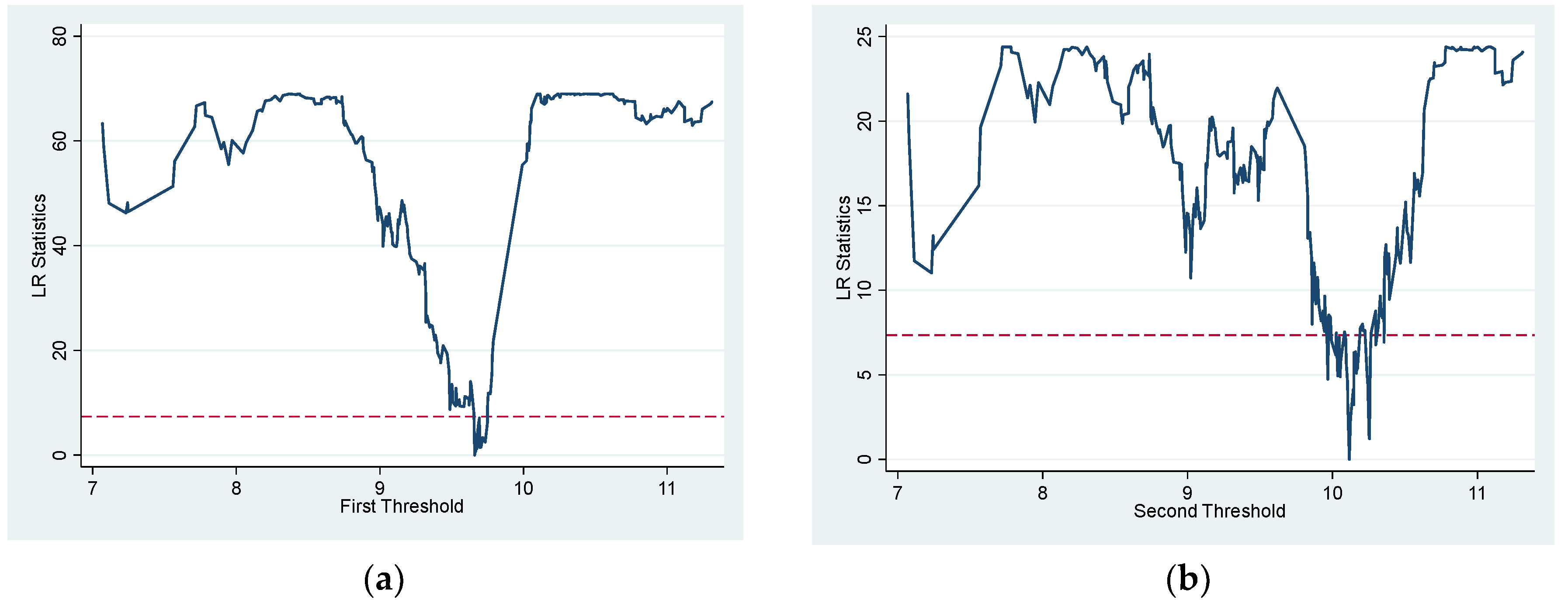
4.4. Analysis of Threshold Effects

There is a complex relationship between financial development, energy consumption, and economic growth [6]. Although energy consumption promotes economic growth, the relationship between them may depend on the importance of financial development. In this paper, the bootstrap method is used for 500 repeated samples, and the panel threshold models are established with financial development and energy consumption as threshold variables. The results are shown in Appendix A with

Table A5. The significance test results for financial development (FD) threshold effects.

Type	F-Value	p-Value	Critical Values			Threshold Estimation Value	95% Asymptotic Confidence Interval
			10%	5%	1%
Single threshold	74.910	0.000	27.575	31.404	50.128	9.705	[9.696, 9.715]
Double threshold	26.670	0.067	24.642	28.215	37.697	9.660	[9.655, 9.665]
						10.116	[10.094, 10.124]

and

Table A6. The significance test results for energy consumption (EC) threshold effects.

Type	F-Value	p-Value	Critical Values			Threshold Estimation Value	95% Asymptotic Confidence Interval
			10%	5%	1%
Single threshold	14.880	0.822	37.520	45.114	65.473	8.032	[7.751, 8.074]
Double threshold	12.470	0.684	30.234	35.228	43.194	8.969	[8.941, 8.972]
						9.892	[9.839, 9.893]

, respectively.

As can be seen from Table A5, the p-value of the single threshold test for FD is 0.000, indicating that FD has threshold effect at the 1% confidence level. The p-value of double threshold test has threshold effect at the 5% confidence level. Therefore, there is a double threshold effect in financial development. The double thresholds are estimated to be 9.660 and 10.116 respectively by using the principle of minimum sum of squares of residuals. As can be seen from Table A6, the p-values of single threshold and double threshold test of EC are 0.822 and 0.684, respectively, which fail the significance test. Therefore, there is no threshold effect in energy consumption.

In order to verify the accuracy of financial development threshold estimation, Figure 3 shows the relationship between threshold estimator and Likelihood Ratio statistic (LR) of FD. As can be seen from Figure 3, the double thresholds for financial development are 9.660 and 10.116 respectively, with confidence intervals of [9.655, 9.665] and [10.094, 10.124]. Within this interval, the likelihood ratio statistic is less than the critical value at the level of 5%. Therefore, it can be considered that the estimate of threshold effect of financial development is real and effective.

On the basis of the threshold test, the panel threshold model needs to be further estimated. The results are shown in

Table 3. Estimation results of panel models.

Variables	Fe (Robust)	Fe (Ordinary)	OLS	EC Threshold	FD Threshold
FD/EC (qit ≤ γ1)				0.283 ***	0.059
FD/EC (γ1 < qit ≤ γ2)				0.288 ***	0.067
FD/EC (qit < γ2)				0.292 ***	0.073 **
lnEC	−0.139 *	−0.139 ***	0.199 **
lnFD	0.306 ***	0.306 ***	0.283 ***
lnK	0.024	0.024	0.244 ***	0.021	0.045 ***
lnL	0.143 ***	0.143 ***	0.524 ***	0.154 ***	0.113 ***
lnOpen	0.003	0.003	0.027 ***	0.006 ***	0.010 ***
lnFis	0.273 ***	0.273 ***	−0.151	0.232 ***	0.457 ***
constant	4.438 ***	4.438 ***	0.373	3.577 ***	3.931 ***
R2	0.984	0.984	0.974	0.985	0.982
F	602.65 ***	135.22 ***	513.67 ***	131.19 ***	129.67 ***

Notes: ***, **, * denote statistical significance levels at 1%, 5% and 10%, respectively.

. In order to enhance the comparison, Table 3 also gives the estimation results of robust fixed effect model, ordinary fixed effect model, OLS model, threshold model with EC as the threshold, and threshold model with FD as the threshold. The robust fixed effect model, ordinary fixed effect model, and OLS model cannot estimate the nonlinear impact of energy consumption on economic growth. The threshold model with EC as threshold variable does not pass the threshold test. Therefore, the threshold model with FD as the threshold variable is selected for analysis. In the FD threshold model, when FD is lower than 9.660, the influence coefficient of energy consumption on economic growth is 0.059. When FD is greater than 9.660 and less than 10.116, the influence coefficient of energy consumption on economic growth is 0.067. When FD is greater than 10.116, the influence coefficient of energy consumption on economic growth is 0.073, which is significant at the level of 5%. It shows that with the rise of financial development, the impact of energy consumption on economic growth is improved by stages. When financial development is greater than 10.116, there is a significant synergistic effect between financial development and energy consumption. Financial development and energy consumption have improved economic growth through reasonable resource allocation. In addition, material capital, labor input, openness, and fiscal expenditure have significant positive effects on economic growth.

5. Conclusions

This paper selects the panel data of 30 provinces in China from 2007 to 2017 as research samples, and uses the spatial econometric analysis method and nonlinear econometric method to analyze the spatial spillover effects and threshold effects of energy consumption and financial development on regional economic growth. The main findings are that China’s regional economic growth presents spatial correlation. In geographical space, it shows spatial agglomeration characteristics of high-high value agglomeration and low-low value agglomeration. Furthermore, the spatial econometric analysis shows that financial development and energy as a production input factor promote China’s economic growth. However, China should also consider the unsustainability of resources and the strong dependence of China’s current economic development on energy. Additionally, energy consumption and financial development have spillover effects on regional economic growth. Finally, the non-linear econometric method finds that with the increasing of financial development, the impact of energy consumption on economic growth is segmented. Through the preceding conclusions, the following policy implications are proposed.

Firstly, energy policies should be tailored to local conditions, optimize the energy consumption structure, and take the road of sustainable development of new energy. After entering the new century, facing the constraints of resources and environment, China has persisted in conserving resources and protecting the environment, and actively transformed the mode of economic development. The Chinese central government has successively promulgated “Action for Energy Development Strategy (2014–2020)”, ”The Revolutionary Strategy for Energy Production and Consumption (2016–2030)”, and other programmatic documents, special documents such as “the Action Plan for Energy Technology Revolution and Innovation (2016–2030)” and “the 13th Five-Year Plan for Renewable Energy Development”. Since the 18th National Congress of the Communist Party of China (CPC), the Chinese government has put forward the strategic thought of “energy revolution” in the face of new trends in international energy development and new changes in energy supply and demand pattern. Due to the difference of regional energy endowment, different provinces have different energy-saving goals. Policy makers should formulate flexible energy revolution policies according to regional energy consumption. The scarcity of resources is bound to limit the rapid growth of China’s economy. Policy makers should vigorously develop new energy to gradually replace traditional energy (such as coal). Meanwhile, policy makers should develop the low-carbon economy and reduce dependence on traditional energy. For example, the production technology with high energy consumption and high pollution will be phased out, and the technical equipment level of environmental protection industry (such as coal gasification technology) will be accelerated.

Secondly, accelerate the construction of multi-level regional financial credit center strategic layout, strengthen regional credit cooperation, and promote the liberalization of financial credit resources. The reason for the spillover effects among regions are the influence of external economies of scale. The free flow of credit among regions is conducive to the rational allocation of financial credit funds in multi-level regional financial credit centers. On one hand, regional comparative advantages should be brought into play to realize differentiated development and healthy competition. On the other hand, policy makers should emphasize the regional coordinated development, realize the financial credit market integration, and then promote the long-term stable growth of regional economy.

Thirdly, rationally allocate energy and financial resources and accelerate the implementation of regional coordinated development. The improvement of the financial development level will increase energy consumption and increase the dependence of economic growth on energy consumption. Financial development and energy consumption have improved economic growth through reasonable resource allocation. Therefore, the financial management department should make full use of financial tools when formulating the financing mechanism, and guide the high energy consumption enterprises to upgrade to the low energy consumption enterprises, so as to realize a coordinated situation of local financial development and energy conservation and emission reduction. The government should actively explore the rational allocation of energy and finance, increase the elimination of excess capacity, strictly implement environmental protection, and production restriction, optimize the energy consumption structure, and accelerate the construction of a resource-saving and environmentally friendly society.

References

1. Zhou, H.; Qu, S.; Wu, Z.; Ji, Y. A study of environmental regulation, technological innovation, and energy consumption in China based on spatial econometric models and panel threshold models. Environ. Sci. Pollut. Res. 2020, 27, 37894–37910. [Google Scholar] [CrossRef] [PubMed]
2. Eren, B.M.; Nigar, T.; Korhan, K.G. The impact of financial development and economic growth on renewable energy consumption: Empirical analysis of India. Sci. Total Environ. 2019, 663, 189–197. [Google Scholar] [CrossRef]
3. National Bureau of Statistics of China. Statistical Communiqué of the People’s Republic of China on the 2019 National Economic and Social Development. National Bureau of Statistics of China website. 2020. Available online: http://www.stats.gov.cn/english/PressRelease/202002/t20200228_1728917.html (accessed on 7 August 2020).
4. Rafindadi, A.A.; Ozturk, I. Effects of financial development, economic growth and trade on electricity consumption: Evidence from post-Fukushima Japan. Renew. Sustain. Energy Rev. 2016, 54, 1073–1084. [Google Scholar] [CrossRef]
5. Shahbaz, M.; Khan, S.; Tahir, M.I. The dynamic links between energy consumption, economic growth, financial development and trade in china: Fresh evidence from multivariate framework analysis. Energy Econ. 2013, 40, 8–21. [Google Scholar] [CrossRef]
6. Shahbaz, M.; Hoang, T.H.V.; Mahalik, M.K.; Roubaud, D. Energy consumption, financial development and economic growth in india: New evidence from a nonlinear and asymmetric analysis. Energy Econ. 2017, 63, 199–212. [Google Scholar] [CrossRef] [Green Version]
7. Khan, S.; Peng, Z.; Li, Y. Energy consumption, environmental degradation, economic growth and financial development in globe: Dynamic simultaneous equations panel analysis. Energy Rep. 2019, 5, 1089–1102. [Google Scholar] [CrossRef]
8. China Statistical Yearbook. Available online: http://www.stats.gov.cn/tjsj/ndsj/ (accessed on 18 September 2020).
9. Wang, S.; Li, Q.; Fang, C.; Zhou, C. The relationship between economic growth, energy consumption, and CO2 emissions: Empirical evidence from China. Sci. Total Environ. 2015, 542 Pt A, 360–371. [Google Scholar] [CrossRef]
10. Liu, Y.; Hao, Y. The dynamic links between CO2, emissions, energy consumption and economic development in the countries along “the belt and road”. Sci. Total Environ. 2018, 645, 674–683. [Google Scholar] [CrossRef]
11. Hao, Y.; Wang, L.; Zhu, L.; Ye, M. The dynamic relationship between energy consumption, investment and economic growth in china\”s rural area: New evidence based on provincial panel data. Energy 2018, 154, 374–382. [Google Scholar] [CrossRef]
12. Acheampong, A.O. Economic growth, CO2 emissions and energy consumption: What causes what and where? Energy Econ. 2018, 74, 677–692. [Google Scholar] [CrossRef]
13. Gozgor, G.; Chi, K.M.L.; Zhou, L. Energy consumption and economic growth: New evidence from the oecd countries. Energy 2018, 153, 27–34. [Google Scholar] [CrossRef] [Green Version]
14. Song, M.; Wang, S.; Yu, H.; Yang, L.; Wu, J. To reduce energy consumption and to maintain rapid economic growth: Analysis of the condition in china based on expended ipat model. Renew. Sustain. Energy Rev. 2011, 15, 5129–5134. [Google Scholar] [CrossRef]
15. Yuan, C.; Liu, S.; Fang, Z.; Xie, N. The relation between Chinese economic development and energy consumption in the different periods. Energy Policy 2010, 38, 5189–5198. [Google Scholar] [CrossRef]
16. Shahbaz, M.; Zakaria, M.; Shahzad, S.J.H.; Mahalik, M.K. The energy consumption and economic growth nexus in top ten energy-consuming countries: Fresh evidence from using the quantile-on-quantile approach. Energy Econ. 2018, 71, 282–301. [Google Scholar] [CrossRef] [Green Version]
17. Aydin, C.; Esen, Ö. Does the level of energy intensity matter in the effect of energy consumption on the growth of transition economies? Evidence from dynamic panel threshold analysis. Energy Econ. 2017, 69, 185–195. [Google Scholar] [CrossRef]
18. Bekun, F.V.; Emir, F.; Sarkodie, S.A. Another look at the relationship between energy consumption, carbon dioxide emissions, and economic growth in South Africa. Sci. Total Environ. 2019, 655, 759–765. [Google Scholar] [CrossRef]
19. King, R.G.; Levine, R. Finance and growth: Schumpeter might be right. Q. J. Econ. 1993, 108, 717–738. [Google Scholar] [CrossRef]
20. Yang, F. The impact of financial development on economic growth in middle-income countries. J. Int. Financ. Mark. Inst. Money 2019, 59, 74–89. [Google Scholar] [CrossRef]
21. Diallo, B.; Al-Titi, O. Local Growth and Access to Credit: Theory and Evidence. J. Macroecon. 2017, 54, 410–423. [Google Scholar] [CrossRef]
22. Wang, C.; Zhang, X.; Ghadimi, P.; Liu, Q.; Lim, M.K.; Stanley, H.E. The impact of regional financial development on economic growth in Beijing–Tianjin–Hebei region: A spatial econometric analysis. Phys. A Stat. Mech. Appl. 2019, 521, 635–648. [Google Scholar] [CrossRef]
23. Sassi, S.; Gasmi, A. The effect of enterprise and household credit on economic growth: New evidence from European union countries. J. Macroecon. 2014, 39, 226–231. [Google Scholar] [CrossRef]
24. Ouyang, Y.; Li, P. On the nexus of financial development, economic growth, and energy consumption in China: New perspective from a GMM panel VAR approach. Energy Econ. 2018, 71, 238–252. [Google Scholar] [CrossRef]
25. Liu, G.; Zhang, C. Does financial structure matter for economic growth in China. China Econ. Review. 2018, 61, 1–19. [Google Scholar] [CrossRef]
26. Law, S.H.; Singh, N. Does too much finance harm economic growth? J. Bank. Financ. 2014, 41, 36–44. [Google Scholar] [CrossRef] [Green Version]
27. Guender, A.V. Credit Prices vs. Credit Quantities as Predictors of Economic Activity in Europe: Which Tell a Better Story? J. Macroecon. 2018, 57, 380–399. [Google Scholar] [CrossRef] [Green Version]
28. Yang, Y. Financial Development and Economic Growth: Based on China’s Financial Development as Threshold Variable. J. Financ. Res. 2014, 404, 59–71. [Google Scholar]
29. Chen, K.C.; Wu, L.; Wen, J. The relationship between finance and growth in china. Glob. Financ. J. 2013, 24, 1–12. [Google Scholar] [CrossRef]
30. Huang, H.C.; Lin, S.C. Non-linear finance–growth nexus: A threshold with instrumental variable approach. Econ. Transit. 2009, 17, 439–466. [Google Scholar] [CrossRef]
31. Al-Mulali, U.; Sab, C.N. The impact of energy consumption and co2 emission on the economic and financial development in 19 selected countries. Renew. Sustain. Energy Rev. 2012, 16, 4365–4369. [Google Scholar] [CrossRef]
32. Komal, R.; Abbas, F. Linking financial development, economic growth and energy consumption in pakistan. Renew. Sustain. Energy Rev. 2015, 44, 211–220. [Google Scholar] [CrossRef]
33. Mirza, F.M.; Kanwal, A. Energy consumption, carbon emissions and economic growth in pakistan: Dynamic causality analysis. Renew. Sustain. Energy Rev. 2017, 72, 1233–1240. [Google Scholar] [CrossRef]
34. Hansen, B.E. Threshold effects in non-dynamic panels: Estimation, testing, and inference. J. Econ. 1999, 93, 345–368. [Google Scholar] [CrossRef] [Green Version]
35. LeSage, J.; Pace, R.K. Introduction to Spatial Econometrics; Peking University Press: Beijing, China, 2014; pp. 50–52. [Google Scholar]
36. Tobler, W.R. A computer movie simulating urban growth in the detroit region. Econ. Geogr. 1970, 46, 234–240. [Google Scholar] [CrossRef]
37. Moran, P.A.P. Notes on continuous stochastic phenomena. Biometrika 1950, 37, 17–23. [Google Scholar] [CrossRef] [PubMed]
38. Anselin, L.; Bera, A.K.; Florax, R.; Yoon, M.J. Simple diagnostic tests for spatial dependence. Reg. Sci. Urban Econ. 1996, 26, 77–104. [Google Scholar] [CrossRef]
Figure 1. Energy consumption, financial development, and gross domestic product of China from 2007 to 2019. Data Sources: China Statistical Yearbook [8].
Energies 13 04982 g001
Figure 2. Scatter plots of Moran’s I of economic growth in China. (a) Description of scatter plots of Moran’s I of economic growth of China in 2008; (b) Description of scatter plots of Moran’s I of economic growth of China in 2011; (c) Description of scatter plots of Moran’s I of economic growth of China in 2014; (d) Description of scatter plots of Moran’s I of economic growth of China in 2017.
Energies 13 04982 g002
Figure 3. Threshold estimator and confidence interval of financial development. (a) The LR function diagram of the first threshold value; (b) The LR function diagram of the second threshold value.
Energies 13 04982 g003