Article

A Coupling Diagnosis Method for Sensor Faults Detection, Isolation and Estimation of Gas Turbine Engines

School of Energy Science and Engineering, Harbin Institute of Technology, Harbin 150001, China
*
Author to whom correspondence should be addressed.
Energies 2020, 13(18), 4976; https://doi.org/10.3390/en13184976
Submission received: 20 August 2020 / Revised: 16 September 2020 / Accepted: 20 September 2020 / Published: 22 September 2020

Abstract

:
In this paper a novel fault detection, isolation, and identification (FDI&E) scheme using a coupling diagnosis method with the integration of the model-based method and unsupervised learning algorithm is proposed and developed for monitoring gas turbine sensor faults, which represents an integration of Square Root Cubature Kalman Filters (SRCKF) and an improved Density-Based Spatial Clustering of Application with Noise (DBSCAN) algorithm. A detection indicator produced by SRCKF with a specific hypothesis is used for extracting sensor fault features against process and measurement noise, as well as operating conditions. Then, an improved DBSCAN is implemented based on a voting scheme to detect and isolate the faulty sensors. Finally, a residual-based fault estimation scheme is proposed to track sensor fault evolution and help to judge the types of faults. Moreover, the observability of the model involved is analyzed to verify the stable operation of the FDI&E scheme. Various experiments for single and concurrent sensor fault scenarios in a dual-spool gas turbine prototype during a whole flight mission are conducted to demonstrate the effectiveness of the proposed FDI&E scheme. Moreover, comparative studies confirm the superiority of our proposed FDI&E scheme than the existing methods in terms of promptness and robustness of the sensor FDI.

1. Introduction

Gas turbine (GT) engines provide power for airplanes, ships and industrial equipment, and reliable and efficient operation is crucial to their safety and performance. Nowadays, various sensors have been equipped in GTs to monitor and control the safe operation of GTs. However, the performance of sensors is very sensitive even when the sensor is a healthy one because sensors are often installed in a very poor working environment of a GT, such as high temperature and high pressure [1]. When the performance of the sensor degenerates, malfunctions, or fails, there will be a serious impact on the follow-up monitoring, control, or fault diagnosis systems, resulting in misdiagnosis, false alarm and even unexpected GT faults that lead to unplanned maintenance of equipment [2]. And the cost of unplanned service interruption is usually significantly higher than the cost of performing preventative maintenance and returning [3]. Hence, a sensor fault detection, isolation, and estimation (FDI&E) scheme is important for the GT safe and stable operation.
Sensor fault diagnosis technology aims to separate the fault information of the sensor through various data processing methods and provide an alarm quickly so as to help the maintenance personnel quickly find out the fault source and eliminate it when the sensor is about to fail or has already failed. Traditionally, the sensor fault diagnosis methods could be categorized into model-based and data-driven methods. In general, model-based methods can be further grouped into basic approaches, namely: (1) Kalman filter (KF)-based [4], (2) parity relations [5], (3) optimization-based algorithms [6], (4) parametric eigenstructure assignment [7] and (5) parameter estimation and identification [8]. The KF-based approach is a popular approach because it not only enables one to detect and isolate sensor faults, but also provides one with information on the magnitude of the fault and its identification information [9,10,11,12,13,14].
Nowadays, KF-based sensor FDI schemes have been successfully designed and tested for GTs. Simani and Spina [15] proposed a sensor FDII strategy based on a linear dynamic system and a bank of KFs in which a set of measured variables of the system is compared with the corresponding signals estimated by filters to generate residual functions that can be used for sensor fault isolation. In the literature [16], an aircraft engine sensor fault diagnostics method with an enhanced bank of KFs is proposed. This approach utilizes a bank of (m + 1) KFs where m is the number of sensors being monitored to simultaneously detect and isolate sensor and component (or actuator) faults. Similarly, in [17] an FDII strategy using a bank of KFs was proposed. Yang et al. [18] proposed an adaptive fault detection and isolation (FDI) framework based on the MM method to detect and isolate sensor faults and gas path faults. Kobayashi and Simon [19] proposed a sensor fault diagnostic system based on a Hybrid Kalman filter (HKF) that is a hybrid of a nonlinear on-board engine model (OBEM) and piecewise linear models, which embedded a nonlinear model in the KF framework to realize the nonlinear estimation. Further, HKF is improved by designing the robust Kalman filter gain matrices through solving two algebraic Riccati equations against both time-varying parameter uncertainties and process and measurement noise [20].
In the majority of the above references systems were designed to detect sensor faults by comparing the outputs of real sensors with the estimated values of corresponding sensors. However, this leads to two problems. One is that few of them have been extended to concurrent sensor fault scenarios, and in the few literature examples related to the field of concurrent sensor FDI, like [10], only two faulty sensors can be detected and the faults must occur at different times. In general, KF-based approaches require one sensor to play two roles at the same time. The first one is that the sensor is used to estimate a correct sensor output value for other sensors. Simultaneously, the output value of this sensor is still used to compare with its redundant information provided by the other sensors to justify whether it is faulty or not. Obviously, these two functions are contrary, where a faulty sensor cannot provide correct redundant information for other faulty sensors, resulting in that only does one sensor act one function that causes the difficulty to realize the concurrent sensor faults detection and isolation.
On the other hand, there exists a big deal of interest in data-driven methods for gas turbine FDI including machine learning-based method [21], neural network-based method [22], fuzzy logic-based method [23] and so on. In general, supervised learning algorithms play an important role in data-driven FDI. However, their application to fault diagnosis problems still leads to several concerns. Firstly and most importantly, supervised learning algorithms depend heavily on labeled samples, so any GT faults not in the labeled sample set may be not detected by the algorithms. Secondly, they might fail to detect slowly varying incipient faults in early stage degradation [24]. Finally, they might only achieve fault classification, but cannot estimate the severity of faults. Unsupervised learning methodologies attempt at investigating mutual dependencies between input and output spaces that are expected to represent more reliable and robust alternatives to supervised methods [25].
This paper proposes a novel coupling diagnosis method with the integration of a model-based method and an unsupervised learning algorithm to accomplish the design and implementation of sensor faults detection, isolation, and estimation (FDI&E) scheme. More specifically, a bank of novel detection indicators produced by Square Root Cubature Kalman Filters (SRCKF) designed with a specific hypothesis is proposed to extract the sensor fault feature and represent the evolution process of sensor faults, which not only is sensitive to the sensor faults but also remains robust concerning process and measurement noise, operating conditions as well as modeling uncertainties. The SRCKF consists of a simple nonlinear state-space model called Corrected Equilibrium Manifold Expansion (CEME) model to cover the entire GT operating regime. Such indicators allow different sensors for monitoring GT measurements to be redundant to each other. And then, an unsupervised learning-based method is implemented for GT sensors FDI, where an improved Density-Based Spatial Clustering of Application with Noise (DBSCAN) algorithm with a voting scheme is proposed for requirements of the sensor FDI scheme. With the consideration that the proposed indicators only carry sensor fault information but the number of fault sensors is unknown, we propose a clustering method to distinguish indicators for health sensors from that for fault sensors. In combination with clustering results a residual-based fault estimation scheme is proposed to track sensor fault evolution. To illustrate the capabilities of our proposed FDI&E scheme, extensive simulation studies are conducted for a dual-spool GT. Firstly, considering the special design of SRCKF used in this paper, an observability analysis experiment is carried out to verify the proposed scheme is feasible during the complex operating conditions of the GT. Then, various single and concurrent sensor fault scenarios under different operating conditions are considered to demonstrate the effectiveness of our proposed FDI&E scheme. Finally, comparative experiments are implemented to indicate the superiority of our proposed FDI&E scheme compared with the existing methods in terms of promptness and robustness of the sensor FDI.
The rest of this paper is organized as follows: In Section 2, the complete FDI&E scheme is introduced. In Section 3, the observability of the CEME model is analyzed. Section 4 introduces the experiment preparation and description. Finally, comprehensive case studies simulations are presented in Section 5. The paper is concluded in Section 6.

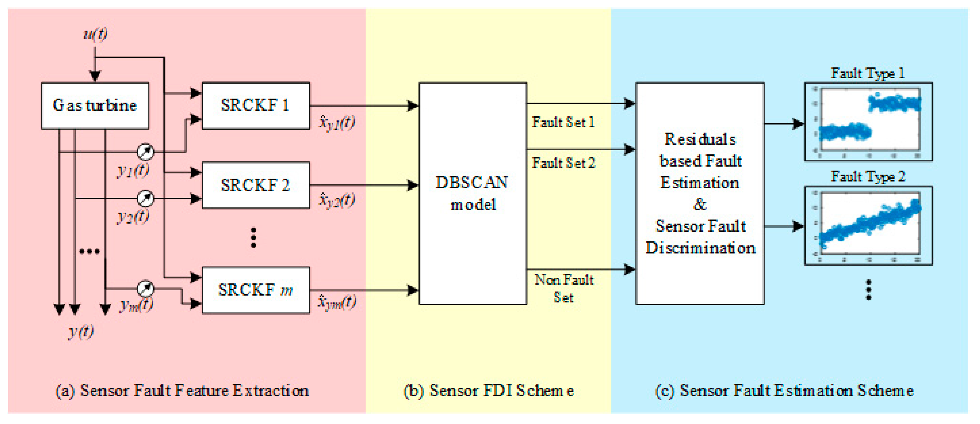
2. Sensor Fault Detection, Isolation and Estimation (FDI&E) Methodology

In this section, a new theoretical framework for the sensor FDI&E methodology is proposed for single and concurrent sensor faults. The framework is divided into three parts. In the first part, a bank of SRCKFs is designed for extracting the feature of sensor faults. In the second part, an improved unsupervised learning algorithm is proposed for sensor FDI. In the last part, a residual-based sensor fault estimation scheme is proposed to track sensor fault evolution. The completed sensor FDI&E scheme is displayed in Figure 1.

2.1. Square Root Cubature Kalman Filter Based Sensor Fault Feature Extraction

A bank of SRCKFs (for a detailed introduction to SRCKF, please refer to Appendix A.1) are designed based on a specific hypothesis that the number of filters is equal to the number of system outputs and each filter is driven by a single output and all the inputs of the system, as shown in Figure 1a. According to the SRCKF basic principle [26], SRCKF is an algorithm that uses the state equations of the nonlinear system to estimate the system state through the input and output observation data. Given that the system is observable, the dimension of system outputs does not affect the estimation of system state by SRCKF. In other words, SRCKF can estimate the system state by using a single output. Such a hypothesis can ensure SRCKFs are independent with each other. The accuracy of each SRCKF to the system state depends on whether the output sensor is normal or fault. Hence, in each SRCKF the optimal estimation value x ^ k of the system state vector shown in Table A1 is designated as a detection indicator. Given that there are m sensors detected in the system, if there are no faulty sensors, indicators estimated by SRCKFs should be approximately consistent with each other. On the contrary, if there is a fault on the i t h output sensor, the corresponding indicator x ^ k is to deviate from the others. And once such a deviation exceeds the pre-specified threshold, a sensor fault is detected.
Such a sensor fault feature extraction logic has some significant advantages. Firstly and most importantly, the proposed indicators allow different sensors such as temperature, pressure and rotor speed sensors to compare with each other by using the proposed detection indicator in order to create an effect similar to physical redundancy. Apparently, in the case that most of the indicators change the same as each other, sensors corresponding to indicators different from the most are faulty. Moreover, since the so-called “the most” is a range and not a specific number, the number of faulty sensors can be arbitrary just under the condition that healthy sensors are in the majority. Considering that it is scarcely possible that the fault type and severity of the sensors are the same as each other, the number of the so-called “the most” can theoretically range from m 1 to 2. In other words, the number of faulty sensors that can be detected ranges from 1 to m 2 . Secondly, the one-to-one form is equivalent to labeling each indicator, which facilitates the isolation of sensor faults. Thirdly, since the proposed scheme just involves the comparison of indicators provided by SRCKFs, it is more sensitive to fault than the method of comparing estimated values with outputs of sensors. Finally, the indicator performed by the SRCKF driven by one output is more susceptible to sensor fault information than that performed by the SRCKF driven by multiple outputs, which further improves the sensitivity of the sensor fault detection. Specific comparative experiments will be carried out in Section 5.3.

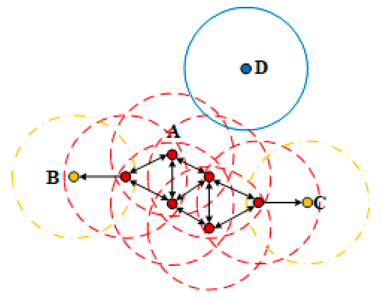
2.2. Density-Based Spatial Clustering of Application with Noise Based Sensors FDI Scheme

From the above section, we know that the proposed indicator x ^ k allows sensors to be redundant to each other. Although the number of faulty sensors and the severity of the fault are unknown, the important known information is that the changes of indicators corresponding to healthy sensors are consistent and the labels of indicators are known. Hence, based on the known information a cluster-based method is proposed for the sensor FDI scheme. The logic is to determine the healthy sensor cluster by the clustering algorithm and then the remains will be determined as the faulty sensors.
Among various clustering techniques (such as K-means [27], BIRCH [28], EM-Clustering [29], and DBSCAN [30]), DBSCAN is selected for the sensor FDI scheme due to its three advantages. The first and most important one is that DBSCAN does not require the number of the clusters to be known a priori, which is suitable for requirements when the occurrence of sensor faults and the number of faulty sensors are random and unknown during the actual operation of GT. Secondly, it is not sensitive to dimensions of input data, which helps improve the applicability of the proposed scheme on different types of GTs (single-spool, dual-spool, or three-spool GTs) with different dimensions of state vectors. Thirdly, as a density-based clustering, it groups data into clusters of arbitrary shapes, even one can be surrounded by another which helps improve the accuracy of the sensor FDI.
DBSCAN is introduced using a minimum density level estimation, based on a threshold for the number of neighbors, Min P t s and the radius   ε . Objects with more than Min P t s neighbors within the radius   ε are considered as a core point. And all neighbors within the radius ε of the core point are considered to be in the same cluster as the core point (also called direct-density reachable). If neighbors are also core points, their neighbors are included by the same cluster (called density reachable). Non-core points are considered as border points, and all points in the same cluster are density connected. Points that do not belong to any cluster are considered as noise points. Figure 2 illustrates the concept of the DBSCAN algorithm, where Min P t s = 4 . The search starts at core point A. B and C are border points, and D is a noise point. Except for D, the remains are within a cluster.
In this paper, the DBSCAN algorithm is properly adjusted for our proposed sensor fault isolation scheme. Consider a set of m points, denoted by D B = { x ^ y 1 , x ^ y 2 , , x ^ y m } that is the set of indicators. And then, DBSCAN defines a cluster using the following notions:
  • Calculate the distance between any x ^ y p , x ^ y q D B that is denoted as d i s ( x ^ y p , x ^ y q ) :
d i s ( x ^ y p , x ^ y q ) = x ^ y p x ^ y q
where ‖·‖ means the Euclidean distance.
  • The ε -neighborhood of x ^ y p , denoted by n b h d ε ( x ^ y p ) , is a subset of D B that   d i s ( x ^ y p , x ^ y q ) ε . The radius ε is the key to ensure correct clustering. If the radius ε is too small, the false alarm rate (FAR) will increase. Conversely, missing alarm rate (MAR) will increase. In this paper, the radius ε is considered as the maximum d i s ( x ^ y p , x ^ y q ) in the training data set where there is no sensor fault.
  • If | n b h d ε ( x ^ y p ) | Min P t s , then x ^ y p is defined as a core point. Min P t s is defined as 1 with the consideration that when only a single sensor fails it also should be in a single cluster. In other words, the concepts of border points and noise points are abandoned in our proposed DBSCAN algorithm.
In the proposed sensor FDI scheme, the proposed DBSCAN algorithm firstly finds all clusters by checking the ε-neighborhood of each point x ^ y p . If | n b h d ε ( x ^ y p ) | Min P t s , then x ^ y p is marked as a core point and a cluster is created. Then, the cluster is expanded by iteratively adding points into the cluster until all points that are direct-density reachable or density reachable are found. And then, it will continue until all points are clustered. Finally, the biggest cluster is selected as the healthy sensor set and the others are considered as the faulty sensor set. Table 1 uses the pseudo code to sketch the completed FDI process.

2.3. Residual-Based Sensor Fault Estimation Scheme

There is no doubt that the estimation of the severity of the sensor faults detected and isolated by the FDI scheme is quite important. Generally, supervised or unsupervised learning algorithms mainly focus on fault classification problem and is not easy to realize the fault estimation. However, in our proposed scheme, due to the integration of the model-based method and unsupervised learning algorithm section, a residual-based methodology is proposed for the sensor fault estimation.
From the above section, we know that indicators are redundant to each other. It means that the indicator corresponding to the healthy sensor can represent the indicator corresponding to the faulty sensor when it is in a healthy state. The severity and trend of sensor fault can be obtained by directly comparing the indicator of the faulty sensor and that of the healthy sensor. Through the FDI scheme, the set of healthy sensors and the set of faulty sensors have been separated. And then, estimation of severity and trend of the sensor fault can be calculated by the following equation:
Δ x ^ f a u l t = x ^ f a u l t x ¯ h e a l t h
where Δ x ^ f a u l t represents the severity of the sensor fault, x ^ f a u l t represents the indicator corresponding to the faulty sensor, x ¯ h e a l t h = ( x ^ 1 + x ^ 2 + + x ^ n ) / n denotes the average of the indicators corresponding to the set of the healthy sensors, n is the number of the healthy sensors.

3. Observability of Corrected Equilibrium Manifold Expansion Model

The prerequisite for the implementation of the proposed sensor FDI&E scheme is that the system is observable. However, the observability of the nonlinear system is an important and difficult research topic, especially the global observability of the general nonlinear system [31], in the area of which there is no satisfactory result so far. Considering the fact that the CEME model instead of the GT physics model is combined with SRCKF, this paper proposes an observability measure based on condition number to qualitatively measure the degree of system observability in order to help judge the reliability of the sensor FDI&E scheme. More details about CEME model are shown in Appendix A.2.
Firstly, for linear systems derived from nonlinear systems, Lee and Markus [32] give the following lemmas:
Lemma 1. 
If the linear system near the equilibrium point of the nonlinear system is completely observable, there is σ > 0 that makes the corresponding nonlinear system observable on γ ( x e , σ ) , where:
γ ( x e , σ ) = { x n | | x x e | σ }
For a CEME model described by Equation (A4), it can be proved that the nonlinear system and corresponding CEME model have the same linearization family. According to the literature [33], CEME model and nonlinear system share the same equilibrium points. Let us assume that:
ζ ( X c e m e , u c e m e ) = A ( α ) ( X c e m e x e ( α ) ) + B ( α ) ( u c e m e u e ( α ) )
Calculate the partial derivative of X c e m e in the function ζ ( X c e m e , u c e m e ) :
ζ ( X c e m e , u c e m e ) X c e m e = A ( α ) X c e m e ( X c e m e x e ( α ) ) + A ( α ) ( X c e m e x e ( α ) ) X c e m e + B ( α ) X c e m e ( u c e m e u e ( α ) ) + B ( α ) ( u c e m e u e ( α ) ) X c e m e = A ( α ) + A ( α ) X c e m e ( X c e m e x e ( α ) ) + B ( α ) X c e m e ( u c e m e u e ( α ) ) ( A ( α ) x e ( α ) α + B ( α ) u e ( α ) α ) α X c e m e
For any equilibrium point of the system, there is the following equation:
ζ ( X c e m e , u c e m e ) X c e m e | x e ( α ) , u e ( α ) = A ( α ) ( A ( α ) x e ( α ) α + B ( α ) u e ( α ) α ) α X c e m e
Meanwhile, the steady state equation of the system is:
f ( x e ( α ) , u e ( α ) ) = 0
Therefore:
A ( α ) x e ( α ) α + B ( α ) u e ( α ) α = 0
Finally:
ζ ( X c e m e , u c e m e ) X c e m e | x e ( α ) , u e ( α ) = A ( α )
Similarly, let us assume the output function of the system as:
ς ( X c e m e , u c e m e ) = Y e ( α ) + C ( α ) ( X c e m e x e ( α ) ) + D ( α ) ( u c e m e u e ( α ) )
In the same way, the partial derivative of output function of the system can be obtained:
ς ( X c e m e , u c e m e ) X c e m e | x e ( α ) , u e ( α ) = C ( α )
It means that parameterized linearization matrices A ( α ) and C ( α ) of the CEME model are the same as those of its original nonlinear system. And it is concluded that the observability of CEME model near the equilibrium point is consistent with that of the nonlinear system.
In this paper, based on the above conclusion, the observability index of linear system by the condition number of matrix defined by Friedland [34] is adjusted to qualitatively measure the degree of CEME system observability with the consideration that parameterized linearization matrices A ( α ) and C ( α ) of the CEME model are available in real time:
η = [ c o n d ( Q ) ] 1 = σ m i n ( Q ) σ m a x ( Q )
where Q = [ C ( α ) C ( α ) A ( α ) C ( α ) ( A ( α ) ) k 1 ] , σ m i n and σ m a x are the minimum and the maximum of the matrix Q singular-value decomposition, k is the dimension of state vector of CEME system. And the smaller η is, the worse the observability of CEME system is.

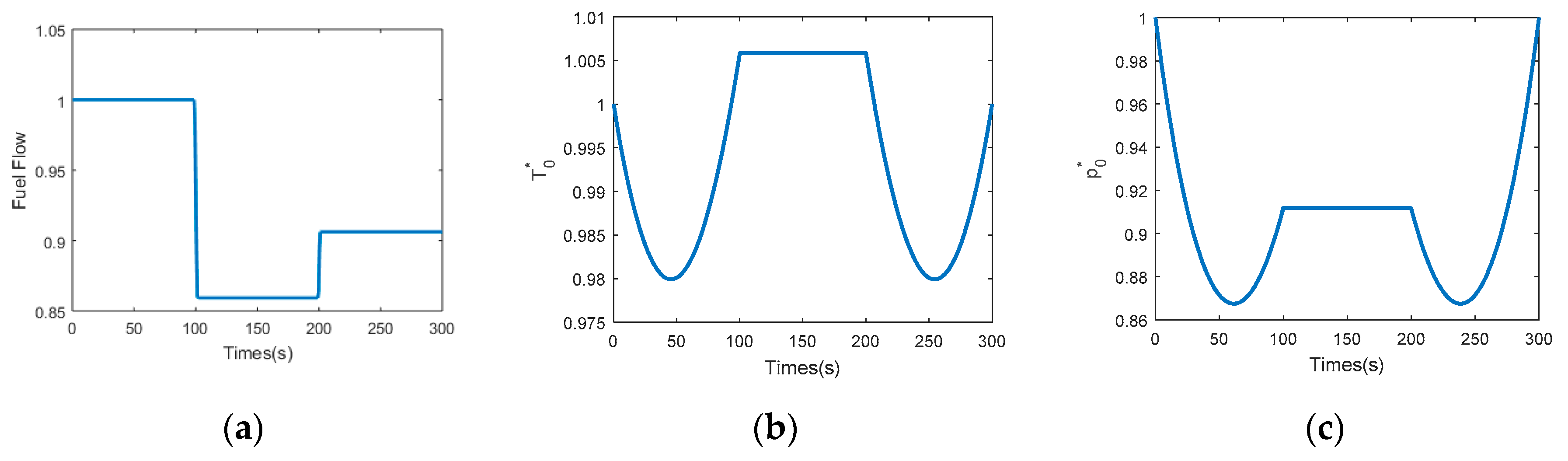
4. Simulation Experiment Preparation and Description

4.1. Experimental Data and Model

In this section, we have used the physics model of a dual-spool GT proposed and verified in [35] to generate the I/O data. In this paper, the GT inputs are GT inlet total temperature T 0 * , GT inlet total pressure p 0 * and fuel flow q m f . Figure 3 describes the changing process of three inputs, where T 0 * and p 0 * are normalized by the reference value of 288.15 K and 101.325 kPa, the fuel flow command signal is normalized by the reference value of 160 L/h. Other GT output variables like the rotor speed, temperature and pressure are normalized by reference values corresponding to engine conditions at 160 L/h fuel flow as well. The GT is simulated for 300 s with a sampling rate of 0.01 s.
Theoretically, all the sensors for the GT gas path measurements can be monitored by our proposed sensor FDI&E scheme. Due to the limited article length, five sensors are selected from different GT components, which are the high pressure turbine rotor speed n h , fan rotor speed n l , the low pressure compressor outlet total temperature T 2 * , the high pressure turbine outlet total temperature T 35 * and the low pressure turbine outlet total pressure   p 4 * . Sensors are affected by the Gaussian noise with standard deviation [ 0.005 0.005 0.01 0.01 0.01 ] T corresponding to the percentages of GT outputs at the standard condition. Figure 4 describes five GT sensor measurements.
The state equations and measurement equations for SRCKF are provided by the CEME model. Considering the actual situation that the GT shaft inertia is much greater than the fluid thermal inertia, the fluid thermal inertia is neglected and n h and n l are specified as state variables of the CEME model, which has been proved to be a reasonable arrangement in literature [35,36]. And then, based on the similarity theory fuel flow q m f , T 0 * and p 0 * constitute the scheduling variable of the CEME model, namely, α = ( q m f T s p s ) / ( p 0 * T 0 * ) . T s and p s are constant corresponding to the known equilibrium manifold (EM). In this paper, they are 288.15 K and 101.325 kPa, respectively. Finally, polynomials of EMs and parametrized Jacobian linearization system matrices scheduled by scheduling variable α are 4 orders and 2 orders, respectively. The CEME modeling process is not described in this paper, which can be found in [33].

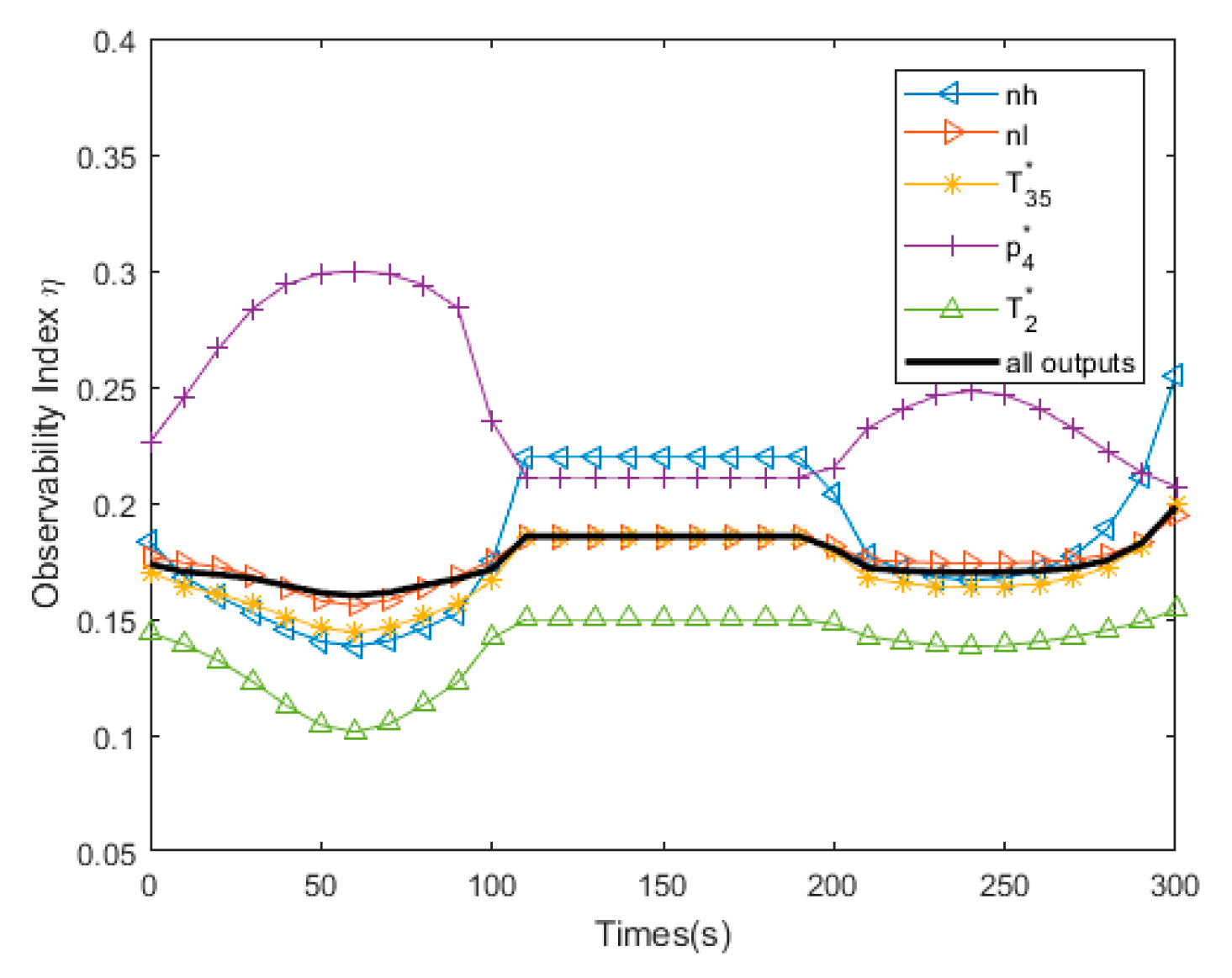
4.2. Observability Analysis of CEME Model

Before implementing our proposed sensor FDI&E scheme, the observability of CEME models during the whole operation process need to be analyzed to ensure that a bank of SRCKFs operate normally. Five CEME models with the same state equations and different measurement equations are built. Besides, another CEME model with all five system outputs is built for the comparative analysis.
Figure 5 shows the observability of six CEME models calculated by Equation (12). Although observability indexes of six CEME models are different from each other, there is no order of magnitude gap between them, which indicates six CEME models are observable. This ensures the stable operation of our proposed FDI&E scheme.

4.3. Determination of Alarm Threshold

Determination of the alarm threshold must weigh the consequences of a false alarm versus the consequences of a missing alarm that might bring about a catastrophic failure [37]. However, FAR and MAR contradict each other. A relatively large alarm threshold can reduce FAR but may increase MAR. There are several factors to affect the alarm threshold, like (1) the process and measurement noise, (2) the modeling errors between the CEME model and the actual engine model and (3) the mismatch between the model and the actual system caused by GT performance degradation. In our paper, such an alarm threshold is equivalent to the distance ε for DBSCAN clustering. And the distance ε is equal to the maximum of the Euclidean distance between indicators x ^ k provided by SRCKFs, it means that the influence of the process and measurement noise on the alarm threshold has been reduced due to the SRCKF filtering. So the modeling errors play a major source of uncertainty in the determination of the alarm threshold. It should be noted that although the mismatch caused by GT performance degradation is also another source of uncertainty, it is not investigated in this paper.
According to the experience of EME modeling from the literature [33,35,36], the maximum modeling error occurs when the system makes a step response that is also the data for building the CEME model. Therefore, the optimal distance ε can be obtained by using the CEME modeling data that can be with the reference to the literature [33]. The final distance ε is 0.0065.

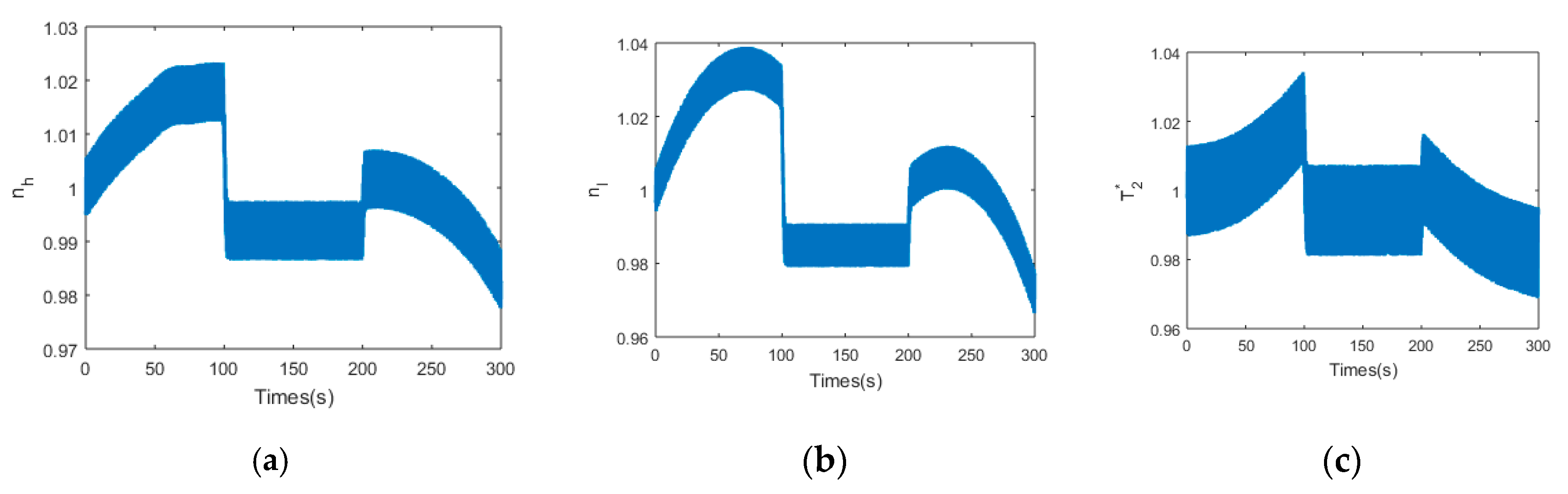
5. Simulation Results

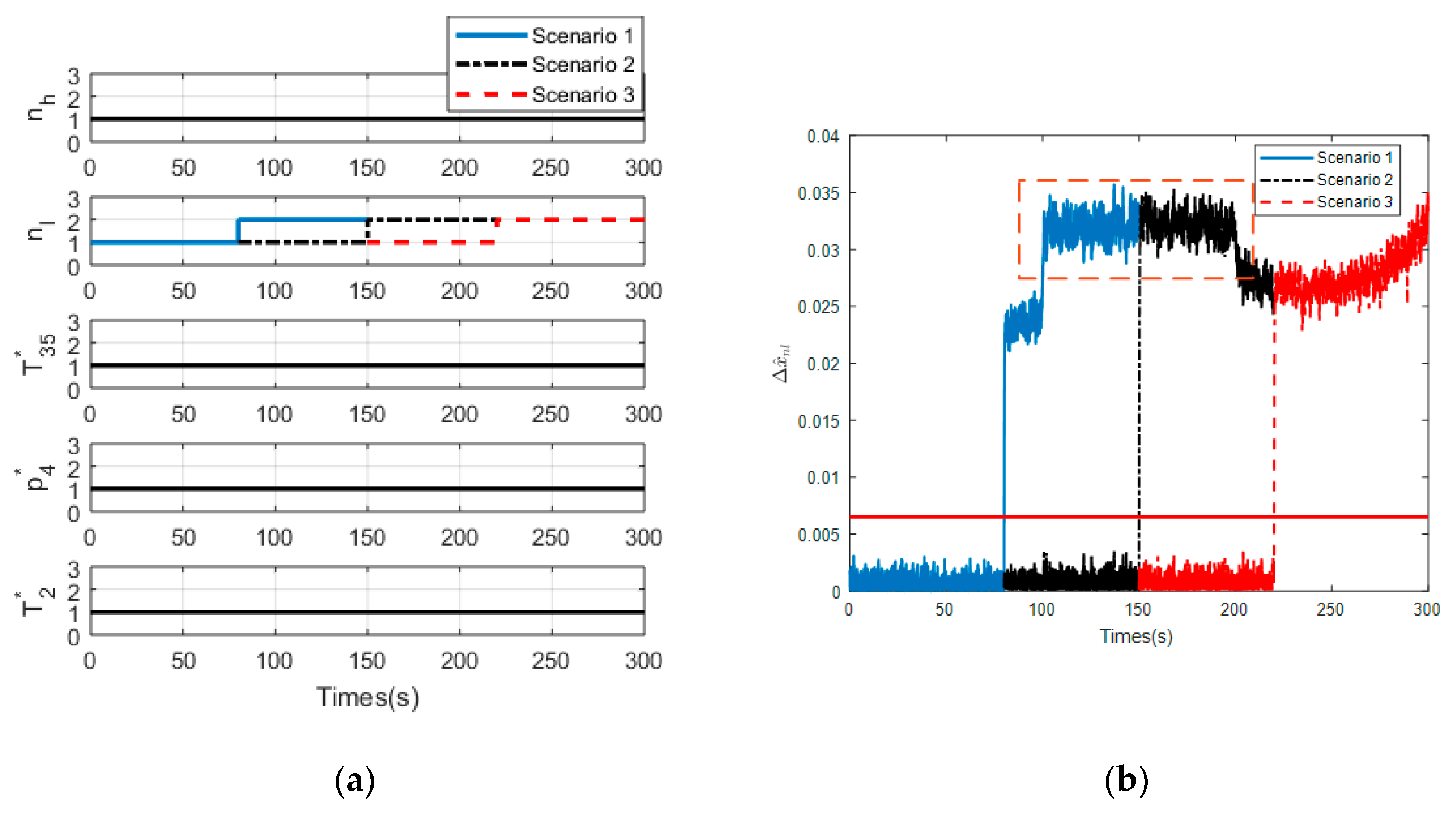
5.1. Single Sensor FDI&E Results

In this section, the performance of the sensor FDI&E scheme with respect to the single sensor fault is evaluated. The evaluation is performed during the whole operation process shown in Figure 3. In this paper, bias fault and drifting Fault are preset on sensors. The maximum deviations of two types of faults are 3% of the GT steady-state output under the standard condition. The severity of drift fault increases linearly from 0% to 3% with a duration of 100 s. The fault occurrence times are set to 80 s, 150 s, and 220 s corresponding to three GT operation scenarios, respectively. At each preset fault occurrence times, both of sensor fault types are preset on each of all five sensors, respectively and detected by our proposed FDI&E scheme. But only FDI&E results for sensor n l are displayed due to article space limitation.
Firstly, experiments corresponding to the bias fault are carried out. Figure 6 shows the results of sensor fault FDI&E scheme corresponding to three scenarios of n l bias fault, where the solid line denotes the sensor fault at 80 s, the chain line denotes the sensor fault at 150 s and the dotted line denotes the sensor fault at 220 s. In addition, the ordinate of Figure 6a represents the label of clusters. According to our proposed FDI scheme, we cluster indicators corresponding to different sensors based on improved DBSCAN to find the biggest cluster in order to mark the remaining clusters as the faulty sensor set.
Figure 6a shows that the healthy sensors n h , T 35 * , p 4 * and T 2 * belong to cluster 1 and the sensor n l belongs to cluster 2. Hence, sensor n l is identified as the faulty sensor. And all three scenarios have the same conclusion, which indicates the new FDI scheme has an ability to accurately and quickly detect and isolate the sensor fault under the influence of operation conditions, various noise and model uncertainty. And then, through the redundant information provided by the healthy sensors, the severity of the faulty sensor n l can be estimated by Equation (2), as shown in Figure 6b. It should be emphasized that the proposed fault estimation scheme can only roughly but not accurately estimate the severity and evolution trend of the sensor fault. The logic of the proposed detection scheme is that the probability density function corresponding to the known measurement equation is different from that corresponding to the output value of the fault sensor. Such a difference makes the optimal estimation state deviate, which is equivalent to mistakenly correcting the probability density function of the original system state. Nevertheless, due to the one-step prediction characteristic of SRCKF, the constant innovation does not change the estimation result of SRCKF, which results in that the fault estimation scheme can still obtain stable estimates in the case of constant GT operating conditions, as shown in the dotted box of Figure 6b. On the contrary, when the operating condition of GT changes, real-time innovation will also modify the probability density function of the state in real time, resulting in that the estimated results vary slightly with the operating conditions. Nevertheless, sensor fault remains the dominant and operating condition will not affect the diagnosis result that will be explained by the following experiment.
Figure 7 shows the results of the sensor fault FDI&E scheme corresponding to three scenarios of n l drifting fault. From Figure 7a, we know that the sensor fault can be still successfully isolated. And it is a normal phenomenon for the deterioration curve to cross the threshold line repeatedly in the process of sensor fault deterioration because the hard threshold is used in this paper. Figure 7b indicates that the proposed fault estimation scheme has an ability to estimate the severity and evolution trend of the sensor fault. Although the estimated indicator corresponding to scenario 1 changes after 180 s following GT operation condition, the influence of sensor fault on the indicator is much greater than that of operation condition and the results. Such a conclusion is further proved by the scenario 2, where the indicator mainly follows with sensor fault rather than with operating conditions in the case of continuous deterioration of the sensor fault shown in the red dotted box of Figure 7b. Therefore, to a certain extent, the proposed sensor fault estimation scheme can help to judge the severity and evolution trend of sensor fault.

5.2. Concurrent Sensors FDI&E Results

In this part, the performance of the sensor FDI&E scheme with respect to the concurrent sensor faults is evaluated. Three faults are set on sensors. Specifically, a bias fault on sensor T 35 * occurs in 80 s, a drifting fault on sensor T 2 * occurs in 80 s, and another bias fault on sensor p 4 * occurs in 90 s. The maximum deviations of two types of faults are the same as that in Section 5.1. The clustering results displayed in Figure 8 show that the healthy sensors n h and n l belong to cluster 1 and faulty sensors belong to cluster 2, cluster 3, and cluster 4, respectively. The results indicate that the proposed FDI scheme has an ability to realize concurrent sensors FDI. After that, the fault estimation scheme is implemented based on the clustering results, which is omitted because it is the same as the results in Section 5.1.

5.3. Comparison Experiments

In this section, the effectiveness of our proposed sensor FDI&E scheme is compared with different existing methods. Various experiments are carried out to compare the robustness toward the GT operating condition and noise and the sensitivity of the FDI scheme to sensor faults.

5.3.1. Robustness Analysis Experiment 1

A comparative experiment between DBSCAN with SRCKF and DBSCAN without SRCKF is implemented. The experimental setup is as follows: The original data is consistent with the above described by Figure 3. A 3% bias fault is added to the sensor n l in 80 s. The first experiment is carried out by our proposed method. In the second experiment, data is only normalized and then clustered only by DBSCAN without SRCKF. The distance ε for DBSCAN without SRCKF is obtained by training the same data as that of Section 5.1. After that, the clustering results are shown in Figure 9.
Our proposed method can isolate the faulty sensor. Comparatively, based on DBSCAN without SRCKF, not only can the sensor faulty not be isolated, but also wrong clustering results appear between 100 s and 200 s. The reason for the above results is that GT output data only normalized include the information on operating conditions and process and measurement noise. In such data, there is an overlap between fault data cluster and normal data cluster, even one cluster is contained by another cluster so that it is difficult for DBSCAN without SRCKF to cluster correctly. On the contrary, in our FDI scheme, the indicators provided by SRCKF can effectively eliminate the effect of operating conditions and noise on clustering, which is equivalent to feature selection of data mining that can expand inter-cluster distance and compress intra-cluster distance to improve the accuracy of clustering.

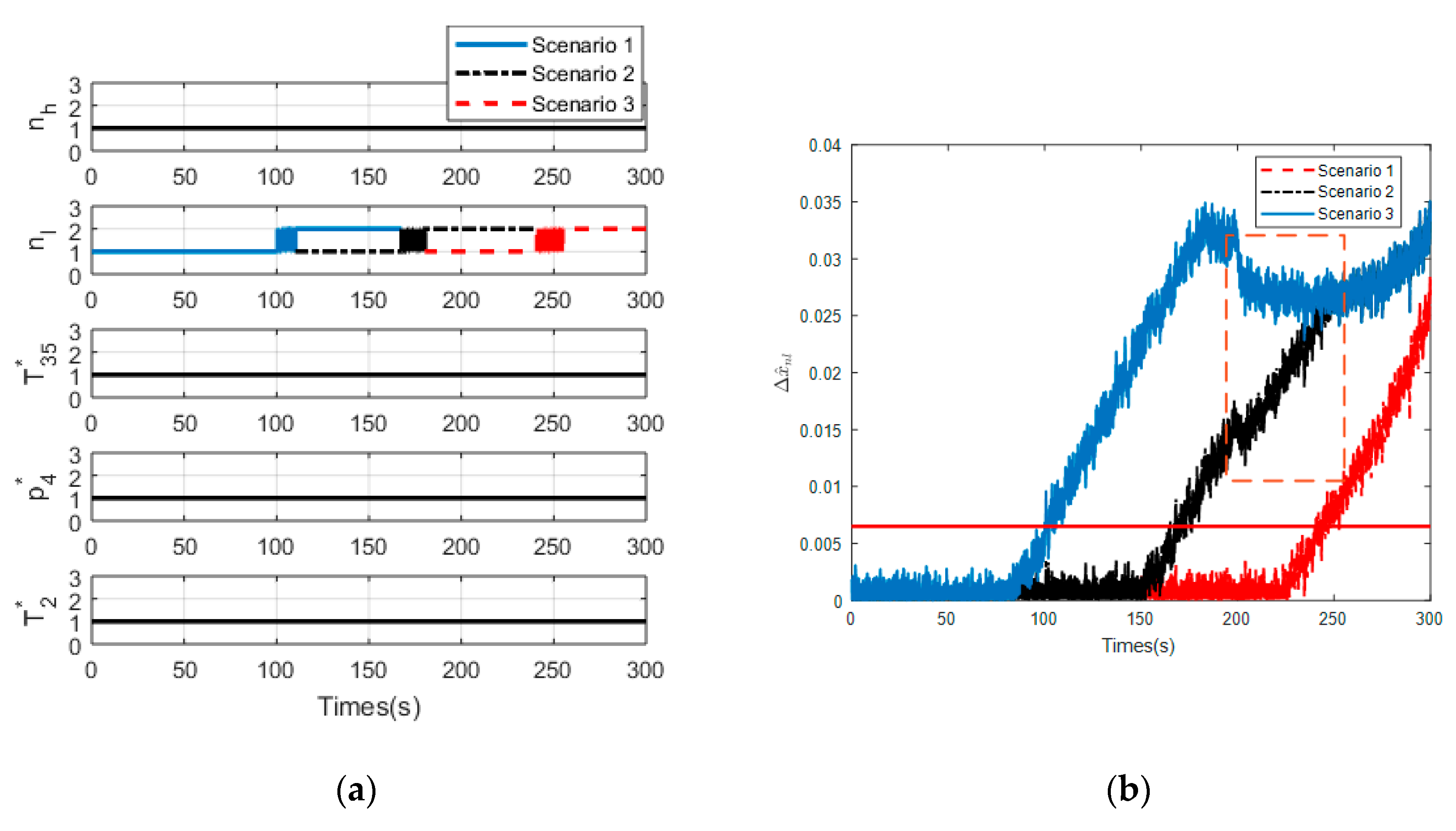
5.3.2. Robustness Analysis Experiment 2

A comparative experiment for sensor n l drifting fault in 80 s between our proposed fault estimation scheme and that proposed by [15] is implemented. The indicator of fault estimation scheme in [15] is the difference between the estimated output and the actual output. However, the alarm threshold is bound to rise to reduce FAR due to the measurement noise. Considering that our fault estimation indicator is system state, not the system output, an additional calculation process to obtain the estimated system output is performed in order to be consistent with the method of [15]. Similarly, one estimated system output with fault information and four ones without fault information are provided. Determination of alarm threshold is almost the same as Section 4.3, but the only difference is that the alarm threshold corresponds to system output instead of system state. After that, the estimated results are shown in Figure 10.
Because the influence of measurement noise on fault estimate has been eliminated by our proposed method, the estimated results still have good robustness under a small alarm threshold. On the contrary, the estimated results with measurement noise frequently cross the alarm line when sensor is in a health state. Hence, it is concluded that our method outperforms the literature [15] in terms of robustness to the measurement noise.

5.3.3. Sensitivity Analysis Experiment

A comparative experiment for sensor p 4 * drifting fault at 80 s between our proposed fault estimation scheme and that proposed by [17] is carried out. The severity of drift fault increases linearly from 0% to 3% with a duration of 100 s. The sensor fault isolation logic of literature [17] is that a bank of Kalman filters are used to detect and isolate sensor fault, each filter is designed using m 1 system outputs for detecting a specific sensor fault. If a fault does occur, all filters except the one using the correct hypothesis will produce large estimation errors, from which a specific fault is isolated. And then, the experiment is carried out and the estimated results are shown in Figure 11.
The design of m 1 system outputs dilutes the fault information where there are always m − 2 healthy sensors and one faulty sensor, like filter 4 ( n h ,   n l ,   p 4 * ,   T 2 * ) and filter 6 ( n h ,   n l ,   T 35 * ,   p 4 * ) displayed in Figure 11 stay below the alarm line during the whole process of sensor failure and the others are less sensitive than that generated by our proposed method. Our proposed method can isolate the sensor fault at 100.97 s when the severity of the sensor fault is only 0.63%. In our FDI&E scheme, each filter is designed using only one output, which can make full use of the influence of sensor error information on system state estimation in order to improve the fault detection promptness.

6. Conclusions

In this paper, a coupling diagnosis method with the integration of a model-based method and unsupervised learning algorithm for sensor faults detection, isolation, and estimation scheme is proposed and developed. In the proposed method, SRCKF and DBSCAN are used for the extraction of the sensor fault features and faulty sensor detection and isolation, respectively. More specifically, a bank of SRCKFs are designed and constructed to produce a unified detection indicator with the aim to extract the sensor fault features, which not only allow different types of sensors to compare with each other, but also suppress the effects of interference including process and measurement noise, and operating conditions on the detection results. Then, an improved DBSCAN algorithm with a voting scheme is proposed for sensor FDI. Finally, a residual-based sensor fault estimation scheme is proposed to estimate the severity and evolution trend of the sensor fault. According to the results, we have illustrated and demonstrated that our proposed sensor FDI&E scheme provides satisfactory performance for diagnosing single or concurrent sensor faults. Further, an observability analysis experiment is carried out to verify the proposed scheme can operate steadily. It is demonstrated through extensive experiments that the promptness and robustness of our proposed approach are significantly superior to those proposed by other investigated methods.
It should be noted that the proposed FDI&E scheme is only verified under the condition that GT components are healthy. And the proposed fault estimation scheme can only roughly but not accurately estimate the severity and evolution trend of the sensor fault. In the future, the research on the coupling of multiple faults including sensor and components as well as the research on accurate sensor fault estimation will be carried out.

Author Contributions

Conceptualization, L.Z. and J.L.; methodology, L.Z.; validation, Y.M.; supervision, W.Z. and D.Y. All authors have read and agreed to the published version of the manuscript.

Funding

This research was funded by NATIONAL NATURAL SCIENCE FOUNDATION OF CHINA, grant number 51976042 and NATIONAL SCIENCE AND TECHNOLOGY MAJOR PROJECT OF CHINA, grant number 2017-I-0007-0008.

Conflicts of Interest

The authors declare no conflict of interest.

Appendix A

Appendix A.1. Square Root Cubature Kalman Filter Algorithm

In the field of KF-based sensor FDI, the modified KFs like Extended Kalman filter (EKF) [38], Unscented Kalman filter (UKF) [39] and Cubature Kalman filter (CKF) [40] are more applicable for nonlinear systems. Among them, CKF that uses a third-degree spherical radial cubature rule to estimate the probability integral of the nonlinear filter has better nonlinear approximation performance, numerical accuracy, and stability compared to EKF and UKF [41]. However, CKF in engineering applications is susceptible to difficulty in decomposing non-semi-definite matrices with Cholesky, which leads to system divergence [42]. In the CKF algorithm, due to the limited calculation step, with the gradual deepening of the filtering calculation, the rounding error of the computer will cause the filtering error covariance matrix and the prediction error covariance matrix to lose the non-negative qualitative and symmetry, and then the calculation of the gain matrix will be distorted, resulting in the divergence of the filter. Meanwhile, the matrix decomposition and matrix inversion in the CKF filtering process will further worsen this phenomenon, resulting in the instability and even divergence of the filtering. To avoid system divergence happening in our FDI&E scheme, SRCKF [26] is used in our paper, where the square root of the state covariance matrix in the form of Cholesky decomposition is directly propagated and updated based on QR-decomposition to guarantee the non-negative qualitative of the covariance matrix. Specifically, QR-decomposition of a matrix A R L × N is given by:
A T = Q × R
where Q N × N is orthogonal, R N × N is upper triangular and N L . The upper triangular part of R , R ˜ , is the transpose of the Cholesky factor of P = A A T , i.e.,   R ˜ T R ˜ = A A T , so that Cholesky decomposition can be replaced by QR-decomposition. And in this paper, q r { · } represents a QR-decomposition of a matrix that only R ˜ is returned.
For a GT system, we firstly define a discrete-time nonlinear dynamic system:
{ x k = f ( x k 1 , u k 1 ) + ω k 1 y k = g ( x k , u k ) + ν k
where u k is a known input vector, x k represent the state of the system, y k is the observed measurement vector, and { ω k } and { ν k }   are process noise and measurement noise, both of which are Gaussian noise with zero means and covariances Q k   and R k , respectively.
And then, the complete specification of SQCKF is given in Table A1, where there are three steps in bold type related to QR-decomposition, and other steps are the same as that of the standard CKF algorithm.
Table A1. SQCKF Algorithm for state estimation.
Initialize with:
x ^ 0 | 0 = E [ x 0 ]   S 0 | 0 = c h o l { E [ ( x 0 x ^ 0 | 0 ) ( x 0 x ^ 0 | 0 ) T ] }
where β = c h o l ( Β ) is the Cholesky decomposition of matrix   Β , Β = β T β , β is an upper triangular matrix, and E ( · ) represents the expectation.
Evaluate the cubature points and time update ( k { 1 , 2 , , } ) :
χ i ,   k 1 | k 1 = S k 1 | k 1 ξ i + x ^ k 1 | k 1
where i = 1 , 2 , , m , m = 2 n , ξ i = m / 2 × [ 1 ] i , [ 1 ] i is the column i of the set [1] that represents
[ 1 ] = [ 1 0 0 0 0 0 0 1 1 0 0 0 0 0 0 1 ] n × m
χ i , k | k 1 = f ( χ i ,   k 1 | k 1 , u k 1 )
x ^ k | k 1 = 1 m i = 1 m χ i , k | k 1
χ k | k 1 = 1 m [ χ 1 , k | k 1 x ^ k | k 1 χ 2 , k | k 1 x ^ k | k 1 χ m , k | k 1 x ^ k | k 1 ]
S k | k 1 = q r { [ χ k | k 1 S Q ,   k 1 ] }  
χ i , k |   k 1 = S k | k 1 ξ i + x ^ k | k 1
χ k |   k 1 = 1 m [ χ 1 , k |   k 1 χ k | k 1 χ 2 , k |   k 1 χ k | k 1 χ m , k |   k 1 χ k | k 1 ]
y i , k |   k 1 = g ( χ i ,   k | k 1 , u k )
y ^ k | k 1 = 1 m i = 1 m y i , k |   k 1
Y k |   k 1 = 1 m [ y 1 , k |   k 1 y ^ k | k 1 y 2 , k |   k 1 y ^ k | k 1 y m , k |   k 1 y ^ k | k 1 ]
Measurement update:
S y y ,   k | k 1 = q r { [ Y k |   k 1 S R ,   k ] }  
P x y , k |   k 1 = χ k |   k 1 Y k |   k 1
P y y , k |   k 1 = S y y ,   k | k 1 S y y ,   k | k 1 T
P y , k |   k 1 = P y y , k |   k 1 R   k
K k = ( P x y , k |   k 1 / S y y ,   k | k 1 T ) / S y y ,   k | k 1
x ^ k = x ^ k | k 1 + K k ( y k y ^ k | k 1 )
S k | k = q r { [ χ k |   k 1 K k Y k |   k 1 K k S R ,   k ] }

Appendix A.2. Corrected Equilibrium Manifold Expansion Model

An accurate nonlinear mathematical model is essential for the SRCKF algorithm. Although analytical models derived from GT physical laws are of the clear physical meaning and the high-order nonlinear dynamic behavior, it is sometimes too hard or even impossible to acquire an exact analytical model due to detailed information on GT components kept secret by manufacturers and only limited information accessible [43]. Thus, in this paper, the CEME model proposed by our previous work [33] is implemented for the sensor FDI&E strategy, which is a model obtained by system identification techniques. The CEME model is improved from the EME model [36] based on the GT similarity theory. While the CEME model retains the advantages (rational, time-saving, and nonlinear) of the EME model, the main improvement of the CEME model is the extension of the model input dimension to meet GT actual demands.
In general, a single-input EME model can be described by the following representation:
{ X ˙ = A ( α ) ( X X e ( α ) ) + B ( α ) ( u u e ( α ) ) Y = Y e ( α ) + C ( α ) ( X X e ( α ) ) + D ( α ) ( u u e ( α ) ) α = p ( X , u )
where X is the state vector,   Y is the output vector,   u   is   the   input   vector ,   X n , Y m , u 1 . A ( α ) , B ( α ) , C ( α ) and D ( α ) are parametrized Jacobian linearization system matrices. The function p is a mapping relationship between α and system variables X and u . The subscript ‘e’ represents the equilibrium point of the system.
The EME modeling procedure has no ability to extend the model input dimension with the restriction of the two-step method of “dynamic and static”. Aiming at the special object of a GT, a CEME model is proposed based on GT similarity theory. For CEME modeling, EM, a set of equilibrium points of a system, is converted to Corrected Equilibrium Manifold (CEM) by incorporating similarity equations. After this transformation, the EME model can be considered as a special CEME model under the fixed GT inlet condition. The CEME model for GT has three inputs including fuel flow, GT inlet total temperature and pressure and can be described as:
{ X ˙ c e m e = A ( α ) ( X c e m e x e ( α ) ) + B ( α ) ( u c e m e u e ( α ) ) Y c e m e = Y e ( α ) + C ( α ) ( X c e m e x e ( α ) ) + D ( α ) ( u c e m e u e ( α ) ) α = p F S C ( X , u , p a , f i x e d * , T a , f i x e d * , p a , i n p u t * , T a , i n p o u t * ) X c e m e = f F S C , 1 ( X , p a , f i x e d * , T a , f i x e d * , p a , i n p u t * , T a , i n p o u t * ) u c e m e = f F S C , 2 ( u , p a , f i x e d * , T a , f i x e d * , p a , i n p u t * , T a , i n p o u t * ) Y = f B S C ( Y c e m e , p a , f i x e d * , T a , f i x e d * , p a , i n p u t * , T a , i n p o u t * ) Subject   to p a , f i x e d * = c o n s t a n t T a , f i x e d * = c o n s t a n t
where p a , f i x e d * and T a , f i x e d * represent the GT inlet condition corresponding to the EM obtained during CEME modeling, p a , i n p u t * and T a , i n p o u t * are inputs of the CEME model, p F S C is a mapping including forward similarity calculation, f F S C , 1 and f F S C , 2 are forward similarity calculation functions and f B S C is a backward similarity calculation function.

References

  1. Liu, J. A dynamic modelling method of a rotor-roller bearing-housing system with a localized fault including the additional excitation zone. J. Sound Vib. 2020, 469, 115144. [Google Scholar] [CrossRef]
  2. Volponi, A.J. Gas turbine engine health management: Past, present, and future trends. J. Eng. Gas Turb. Power 2014, 136, 051201. [Google Scholar] [CrossRef]
  3. Holcomb, C.M.; de Callafon, R.A.; Bitmead, R.E. Closed Loop Nonlinear System Identification Applied to Gas Turbine Analytics. Turbo Expo Power Land Sea Air 2014, 45752, V006T06A013. [Google Scholar]
  4. Frank, P.M. Fault diagnosis in dynamic systems using analytical and knowledge-based redundancy: A survey and some new results. Automatica 1990, 26, 459–474. [Google Scholar] [CrossRef]
  5. Isermann, R.; Balle, P. Trends in the application of model-based fault detection and diagnosis of technical processes. Control Eng. Pr. 1997, 5, 709–719. [Google Scholar] [CrossRef]
  6. Hwang, I.; Kim, S.; Kim, Y.; Seah, C.E. A survey of fault detection, isolation, and reconfiguration methods. IEEE Trans. Control Syst. Technol. 2010, 18, 636–653. [Google Scholar] [CrossRef]
  7. da Silva, J.C.; Saxena, A.; Balaban, E. A knowledge-based system approach for sensor fault modeling, detection and mitigation. Expert Syst. Appl. 2012, 39, 10977–10989. [Google Scholar] [CrossRef]
  8. Gao, Z.; Cecati, C.; Ding, S.X. A survey of fault diagnosis and fault-tolerant techniques—Part I: Fault diagnosis with model-based and signal-based approaches. IEEE Trans. Ind. Electron. 2015, 62, 3757–3767. [Google Scholar] [CrossRef] [Green Version]
  9. Salahshoor, K.; Mosallaei, M.; Bayat, M. Centralized and decentralized process and sensor fault monitoring using data fusion based on adaptive extended Kalman filter algorithm. Measurement 2008, 41, 1059–1076. [Google Scholar] [CrossRef]
  10. Pourbabaee, B.; Meskin, N.; Khorasani, K. Sensor fault detection, isolation, and identification using multiple-model-based hybrid Kalman filter for gas turbine engines. IEEE Trans. Control Syst. Technol. 2015, 24, 1184–1200. [Google Scholar] [CrossRef] [Green Version]
  11. Zarei, J.; Shokri, E. Robust sensor fault detection based on nonlinear unknown input observer. Measurement 2014, 48, 355–367. [Google Scholar] [CrossRef]
  12. Lu, F.; Lv, Y.; Huang, J. A model-based approach for gas turbine engine performance optimal estimation. Asian J. Control 2013, 15, 1794–1808. [Google Scholar] [CrossRef]
  13. Li, L.L.; Zhou, D.H.; Wang, Y.Q. Unknown input extended Kalman filter and applications in nonlinear fault diagnosis. Chin. J. Chem. Eng. 2005, 13, 783–790. [Google Scholar]
  14. Cao, M.; Qiu, Y.; Feng, Y. Study of wind turbine fault diagnosis based on unscented Kalman filter and SCADA data. Energies 2016, 9, 847. [Google Scholar] [CrossRef]
  15. Simani, S.; Spina, P.R. Kalman filtering to enhance the gas turbine control sensor fault detection. Theory Pract. Control Syst. 1998, 443–450. [Google Scholar] [CrossRef]
  16. Kobayashi, T.; Simon, D.L. Evaluation of an enhanced bank of Kalman filters for in-flight aircraft engine sensor fault diagnostics. J. Eng. Gas Turb. Power 2005, 127, 497–504. [Google Scholar] [CrossRef] [Green Version]
  17. Xue, W.; Guo, Y.; Zhang, X. A bank of kalman filters and a robust kalman filter applied in fault diagnosis of aircraft engine sensor/actuator. In Proceedings of the Second International Conference on Innovative Computing, Informatio and Control (ICICIC 2007), Kumamoto, Japan, 5–7 September 2007. [Google Scholar]
  18. Yang, Q.; Li, S.; Cao, Y. Multiple model-based detection and estimation scheme for gas turbine sensor and gas path fault simultaneous diagnosis. J. Mech. Sci. Technol. 2019, 33, 1959–1972. [Google Scholar] [CrossRef]
  19. Kobayashi, T.; Simon, D.L. Hybrid Kalman filter approach for aircraft engine in-flight diagnostics: Sensor fault detection case. Turbo Expo Power Land Sea Air 2006, 42371, 745–755. [Google Scholar]
  20. Pourbabaee, B.; Meskin, N.; Khorasani, K. Robust sensor fault detection and isolation of gas turbine engines subjected to time-varying parameter uncertainties. Mech. Syst. Signal Pr. 2016, 76, 136–156. [Google Scholar] [CrossRef]
  21. Sun, R.Z.; Shi, L.C.; Yang, X.L. A coupling diagnosis method of sensors faults in gas turbine control system. Energy 2020, 205, 117999. [Google Scholar] [CrossRef]
  22. Liu, J.; Liu, J.; Yu, D. Fault detection for gas turbine hot components based on a convolutional neural network. Energies 2018, 11, 2149. [Google Scholar] [CrossRef] [Green Version]
  23. Sun, X.L.; Wang, N. Gas turbine fault diagnosis using intuitionistic fuzzy fault Petri nets. J. Intell. Fuzzy Syst. 2018, 34, 1–9. [Google Scholar] [CrossRef]
  24. Hu, J.; Zhang, L.; Liang, W. Dynamic degradation observer for bearing fault by mts-som system. Mech. Syst. Signal Pr. 2013, 36, 385–400. [Google Scholar] [CrossRef]
  25. Shen, Y.; Khorasani, K. Hybrid multi-mode machine learning-based fault diagnosis strategies with application to aircraft gas turbine engines. Neural Netw. 2020, 130, 126–142. [Google Scholar] [CrossRef] [PubMed]
  26. Arasaratnam, I.; Haykin, S. Cubature kalman filters. IEEE Trans. Autom. Control 2009, 54, 1254–1269. [Google Scholar] [CrossRef] [Green Version]
  27. Likas, A.; Vlassis, N.; Verbeek, J.J. The global k-means clustering algorithm. Pattern Recogn. 2003, 36, 451–461. [Google Scholar] [CrossRef] [Green Version]
  28. Cleophas, T.J. Machine learning in therapeutic research: The hard work of outlier detection in large data. Am. J. Ther. 2016, 23, e837–e843. [Google Scholar] [CrossRef]
  29. Sharma, A.; Kamola, P.J.; Tsunoda, T. 2D–EM clustering approach for high-dimensional data through folding feature vectors. BMC Bioinform. 2017, 18, 547. [Google Scholar] [CrossRef]
  30. Schubert, E.; Sander, J.; Ester, M. DBSCAN revisited, revisited: Why and how you should (still) use DBSCAN. ACM T Database Syst. 2017, 42, 1–21. [Google Scholar] [CrossRef]
  31. Bartosiewicz, Z. Local observability of nonlinear systems. Syst. Control Lett. 1995, 25, 295–298. [Google Scholar] [CrossRef]
  32. Lee, E.B.; Markus, L. Foundations of Optimal Control Theory; Minnesota University Minneapolis Center for Control Sciences: Minneapolis, MN, USA, 1967. [Google Scholar]
  33. Zhu, L.; Liu, J.; Zhou, W. An improvement method based on similarity theory for equilibrium manifold expansion model. In Proceedings of the 2019 IEEE International Conference on Power Data Science (ICPDS), Taizhou, China, 12–15 December 2019; pp. 105–108. [Google Scholar]
  34. Friedland, B. Controllability Index Based on Conditioning Number. J. Dyn. Syst. Meas. Control 1975, 97, 444. [Google Scholar] [CrossRef]
  35. Yu, D.; Zhao, H.; Xu, Z. An approximate non-linear model for aeroengine control. Proc. Inst. Mech. Eng. Part G 2011, 225, 1366–1381. [Google Scholar] [CrossRef]
  36. Zhao, H.; Liu, J.; Yu, D. Approximate nonlinear modeling and feedback linearization control for aeroengines. J. Eng. Gas Turb. Power 2011, 133, 111601. [Google Scholar] [CrossRef]
  37. Li, F.; Zhou, G.; Li, X. A symbolic reasoning based anomaly detection for gas turbine subsystems. In Proceedings of the 2017 Prognostics and System Health Management Conference (PHM-Harbin), Harbin, China, 9–12 July 2017; pp. 1–8. [Google Scholar]
  38. Foo, G.H.B.; Zhang, X.; Vilathgamuwa, D.M. A sensor fault detection and isolation method in interior permanent-magnet synchronous motor drives based on an extended Kalman filter. IEEE Trans. Ind. Electron. 2013, 60, 3485–3495. [Google Scholar] [CrossRef]
  39. Julier, S.J.; Uhlmann, J.K. Unscented filtering and nonlinear estimation. Proc. IEEE 2004, 92, 401–422. [Google Scholar] [CrossRef] [Green Version]
  40. Li, W.; Jia, Y. Location of mobile station with maneuvers using an IMM-based cubature Kalman filter. IEEE Trans. Ind. Electron. 2011, 59, 4338–4348. [Google Scholar] [CrossRef]
  41. Yan, L.; Zhang, Y.; Xiao, B. Fault detection for nonlinear systems with unreliable measurements based on hierarchy cubature Kalman filter. Can. J. Chem. Eng. 2018, 96, 497–506. [Google Scholar] [CrossRef]
  42. Chen, X.; Shen, W.; Dai, M. Robust adaptive sliding-mode observer using RBF neural network for lithium-ion battery state of charge estimation in electric vehicles. IEEE Trans. Veh. Technol. 2015, 65, 1936–1947. [Google Scholar] [CrossRef]
  43. Kim, T.S. Model-based performance diagnostics of heavy-duty gas turbines using compressor map adaptation. Appl. Energy 2018, 212, 1345–1359. [Google Scholar]
Figure 1. Sensor FDI&E scheme based on SRCKF and DBSCAN.
Energies 13 04976 g001
Figure 2. Illustration of the DBSCAN algorithm.
Energies 13 04976 g002
Figure 3. Profiles of (a) fuel flow, (b) GT inlet total temperature T 0 * , and (c) GT inlet total pressure p 0 * .
Energies 13 04976 g003
Figure 4. Profiles of (a) the high pressure turbine rotor speed n h , (b) fan rotor speed n l , (c) the low pressure compressor outlet total temperature T 2 * , (d) the high pressure turbine outlet total temperature T 35 * and (e) the low pressure turbine outlet total pressure   p 4 * .
Energies 13 04976 g004aEnergies 13 04976 g004b
Figure 5. Observability indexes of five CEME model with single output and one with all outputs.
Energies 13 04976 g005
Figure 6. Three scenarios of n l bias fault of (a) FDI scheme and (b) fault estimation scheme.
Energies 13 04976 g006
Figure 7. Three scenarios of n l drifting fault of (a) FDI scheme and (b) fault estimation scheme.
Energies 13 04976 g007
Figure 8. FDI for the scenario of concurrent sensor faults.
Energies 13 04976 g008
Figure 9. The contrast experiment between our proposed DBSCAN and the general DBSCAN.
Energies 13 04976 g009
Figure 10. The robustness of our proposed method against measurement noises.
Energies 13 04976 g010
Figure 11. Comparison test of sensor FDI for   p 4 * drifting fault.
Energies 13 04976 g011
Table 1. Sensor FDI process based on DBSCAN.
Input: D B = { x ^ y 1 , x ^ y 2 , , x ^ y m } , ε , Min P t s
Output: Each x ^ y i is associated with a label (faulty sensor or healthy sensor)
BEGIN
clusterID = 0;
for unvisited point x ^ y p in D B do
{
 mark x ^ y p as visited;
n b h d ε ( x ^ y p ) = GetNeighborhood( x ^ y p , ε );
 clusterID.   x ^ y p = clusterID; // create a cluster containing x ^ y p
 flag.   x ^ y p = core;
 for x ^ y q in n b h d ε ( x ^ y p ) do
 {
  if x ^ y q is unvisited then
 {
   mark x ^ y q as visited;
 clusterID.   x ^ y q = clusterID;
n b h d ε ( x ^ y q ) = GetNeighborhood( x ^ y q , ε );
 if size ( n b h d ε ( x ^ y q ) ) Min P t s then
 {
 flag.   x ^ y q =core;
n b h d ε ( x ^ y q ) =Union ( n b h d ε ( x ^ y q ) , n b h d ε ( x ^ y q ) ) ;
 }
 }
 }
 clusterID = clusterID + 1;
}
Select the biggest cluster and mark points within it as healthy sensors;
Select the other clusters and mark points within them as faulty sensors;
END

