Next Article in Journal
Predicting Temperature of Permanent Magnet Synchronous Motor Based on Deep Neural Network
Next Article in Special Issue
Residential Natural Gas Demand Response Potential during Extreme Cold Events in Electricity-Gas Coupled Energy Systems
Previous Article in Journal
Demand-Response Application in Wastewater Treatment Plants Using Compressed Air Storage System: A Modelling Approach
 
 
Correction published on 16 June 2023, see Energies 2023, 16(12), 4752.
Article

A Comparison of Various Bottom-Up Urban Energy Simulation Methods Using a Case Study in Hangzhou, China

1
School of Architecture, Southeast University, Nanjing 210096, China
2
Key Laboratory of Urban and Architectural Heritage Conservation, Ministry of Education, Nanjing 210096, China
3
The Bartlett School of Construction and Project Management, University College London, London WC1E7HB, UK
4
College of Architecture and Urban Planning, Tongji University, Shanghai 200092, China
5
Key Laboratory of Ecology and Energy-Saving Study of Dense Habitat (Tongji University), Ministry of Education, Shanghai 200092, China
*
Author to whom correspondence should be addressed.
Energies 2020, 13(18), 4781; https://doi.org/10.3390/en13184781
Submission received: 22 August 2020 / Revised: 7 September 2020 / Accepted: 9 September 2020 / Published: 14 September 2020 / Corrected: 16 June 2023
(This article belongs to the Collection Demand Management for Buildings and Industrial Facilities)

Abstract

:
Urban energy simulation can provide valuable information to urban planning, urban energy management, and urban emission reduction. Therefore, urban energy simulation has become an active research discipline. Various urban energy simulation methods and techniques have been developed and applied to cities on different scales. A review is conducted to categorize these methods and techniques and to analyze their pros and cons. Several representative methods and techniques are compared for their data inputs, suitable scales, accuracy, and computing speeds. Hangzhou South Railway Station area, which contains 522 buildings, is used as the case to evaluate the effectiveness and challenges of different urban energy simulation methods.

1. Introduction

It is already well known that carbon dioxide is a major contributor to global climate change [1]. CO2 emissions from human activities have been increasing globally since the late 18th century [2]. Cities, due to their high levels of population and human activities produce an enormous amount of carbon dioxide as well as other emissions such as HC and nitrogen oxides. Another existing trend is that more people from rural areas are now moving into cities to improve their living quality [3]. According to data collected in 2014, 54% of the global population were living in cities, and this number is predicted to increase to 66% by 2050 [4]. With the current prevailing population growth and urbanization rate, by 2030, the global urban area will triple compared with that at the beginning of the 20th century [5]. Linking these two developments, human activities in urban areas now constitute the primary source of anthropogenic greenhouse gas emissions [6]. Due to this phenomenon, cities are consuming over three-quarters of society’s primary energy [7,8,9], with urban emissions accounting for 75% of overall global carbon dioxide emissions [10]. Within cities, buildings are one of the top energy consumers (accounting for over 40% of energy consumption and one-third of greenhouse gas emissions) [11,12]. Therefore, it is extremely important to have a better understanding of how buildings in cities are using energy, and a popular method to achieve this is the use of urban energy simulation models [13,14,15,16,17,18].
The urban energy simulation model is a valuable and powerful tool for calculating, visualizing, and analyzing the energy consumption of buildings at either district or urban levels [19]. It enhances the development of green, ecological, and low-carbon urban planning and also provides guidance on developing urban energy management policies [20]. Urban energy simulation models only started to be used some years ago [21]. However, due to the urgent requirement of reducing urban energy consumption, they have captured the attention of researchers [21]. When using this method, dynamic building performance simulation packages, such as EnergyPlus [22], TRANSYS [23], and DOE-2 [24], are commonly adopted for calculating the energy consumption of individual buildings, and the calculation results are then allocated to urban/district scales to show the energy distribution of buildings within the area under investigation [25].
When developing urban energy simulation models, several approaches have been adopted by researchers and, basically, they can be classified as either top-down [26] or bottom-up [27]. The top-down approach uses macro-statistical data to estimate the urban energy consumption of overall industrial and administrative areas, treating the buildings within an area as a single energy entity. Therefore, it cannot reflect the different levels of energy performance between individual buildings. This approach calculates the urban energy consumption through a long-term relationship between the energy use of possible major drivers, such as GDP, energy price, population, household size, technologies and practices, and weather conditions [28,29,30]. According to whether energy data is the only data type required for calculating urban energy consumption, this approach can be divided into statistical methods or other methods, and the statistical analysis method can be further classified into many sub-methods, such as the economic variables method and the physical variables method [31]. The bottom-up approach simulates urban energy consumption based on the calculated energy consumption of individual buildings within the area [32]; therefore, it can better reflect the spatial energy distribution and has a higher accuracy than the top-down approach [28]. Based on how the energy consumption of individual buildings is calculated, this approach can be further classified as a physical model method, data-driven model method, or hybrid model method [27], where the physical model method is used most commonly due to its transparency in modeling building energy consumption and its capability to link calculated urban energy simulation with urban morphological aspects, such as building archetypes. This method can be further classified as an archetype method or detailed model method, depending on whether archetype buildings are used to represent hundreds or even thousands of buildings within the area. Figure 1 depicts this basic classification of urban energy simulation methodology.
In urban energy simulations, there may be some major challenges. Firstly, the computational load required is significantly higher than that needed to simulate individual buildings, as an urban energy simulation task often involves hundreds or even thousands of buildings. Secondly, the information and data required for conducting an urban energy simulation are multi-dimensional and difficult to collect. Thirdly, conducting an urban energy simulation often involves multiple program packages and cross-platform operations [33]. Additionally, due to the existence of different methods to do this task, as introduced above, it is important to understand the performance of each method and identify its advantages and disadvantages. This will greatly help when selecting the most appropriate method in real applications. Due to the better representation of spatial distribution and the higher accuracy of the bottom-up approach, it was specifically considered in this study. Section 2 of this paper introduces some basic knowledge about the bottom-up approach and its sub-methods. Section 3 presents the basic methodology used in this study, including a field case study with 522 buildings and model development processes. Section 4 compares the results simulated by different methods from three different angles, namely urban energy consumption patterns, dynamic nature, and simulation performance, and provides appropriate discussions. At the end, the major findings from this study are presented, with discussions on possible policy implications.

2. Bottom-Up Approach for Urban Energy Simulation

Top-down approaches have a fast processing speed and are easy to integrate with policies, but they cannot be combined with the spatial form and have a low level of accuracy. The top-down approach often employs energy-economy interactions to estimate urban energy consumption. Bentzen and Engsted [34] used a simple regression model to simulate Danish energy consumption. They found a close coupling relationship between energy consumption, household income, and energy prices. In addition to economic variables, some top-down models also consider physical factors such as weather or climatic conditions. Zhang [35] incorporated climate change to calculate and compare residential energy consumption in China, Japan, the United States, and Canada. They combined the energy consumption of electricity, coal gas, liquefied petroleum gas, and natural gas to estimate residential energy consumption. The bottom-up approach simulates urban energy at the building level, which is easy to combine with the spatial form and has a higher level of accuracy. The bottom-up approach includes three methods, namely, the physical model method, the hybrid method, and the data-driven method.

2.1. Physical Model Method

The physical model method is the most commonly used bottom-up approach to model urban energy. The simulation relies on a building thermal model to calculate the energy consumption or load of individual buildings and then integrates these factors to obtain the corresponding information at the urban level [36]. Typical representative methods are the archetype model method and the detailed model method [31,36].
Reinhart [37] used the archetype model method to calculate the energy consumption in Boston. In the archetype model method, the energy consumption calculation of the individual building follows a complex, dynamic, and detailed model, and massive urban buildings are summarized into several architectural prototypes with common energy consumption rules, thereby calculating the building energy consumption of the entire city [31]. Chen et al. used the City Building Energy Saver (CityBES) method to simulate urban energy consumption in San Francisco. In the CityBES model, the energy consumption calculation of an individual building is done using a complex, dynamic, and sophisticated model to simulate all urban buildings within the study area, and each building is modeled respectively [12,31]. Another detailed model method, also referred to as the 3D CityGML method, which is introduced below, is a city energy consumption simulation method based on the CityGML data set method that can simulate comprehensive urban information [38,39].
The physical model method uses existing technical knowledge as the input, such as building type, building area, building geometry and non-geometric information. At present, the main challenges are the following three points: First of all, the basic data on urban buildings are difficult to obtain. The basic data on urban buildings include the shape of the building, the height, the heat transfer coefficient of the envelope, and the ratio of the window. The non-geometric information, such as the heat transfer coefficient of the envelope required in the modeling process, is difficult to obtain. The second challenge is that there is currently no software available for urban energy simulation. The biggest difficulty in software development is determining how to couple urban building geometry information, non-geometric information, and energy simulation software [3]. Third, no scholars have studied the simulation speed and accuracy of different urban energy consumption simulation methods at different city scales, thus providing a selective reference for urban designers.

2.2. Data-Driven Model Method

The data-driven model method uses the statistical regression method to obtain a calculation model for urban energy consumption at the very foundation of the measured energy consumption data. This method is a relatively accurate prediction model. However, depending on the quantity and quality of measured data, the scalability is limited, and it is difficult to integrate the model with urban planning and urban design [36,40,41].
Based on the analysis and processing of the measured data, Jimeno and Arno [36] used the data-driven model method to calculate the energy consumption requirements of each building. This method can simulate the energy consumption of building groups without loss. Moreover, the energy consumption simulation results of each building can be compared with the energy consumption information displayed in the current statistics. Parti [42] analyzed the residential electricity use in San Diego. In this study, regression methods were used to estimate the utilization rate of residential appliances (such as dishwashers, freezers, and televisions). Thus, the level of energy consumption was projected by surveys of 5286 households and utilities that provided monthly electric billing data. The artificial intelligence method predicts energy consumption, which consists of four parts: data collection, data preprocessing, model training, and model testing [43]. The artificial neural network (ANN) is a common artificial intelligence method for predicting urban energy consumption [12,44]. The ANN [45] is a mathematical model that uses historical data to represent the performance of the system, which simulates the biological neural network. Supervised learning is the most common method used in the literature of building energy prediction [46].
The data-driven model method bridges the gap between detailed individual energy consumption and regional or national econometric indicators. The main limitation of the data-driven model method is that it cannot be combined with the spatial change of an urban area because of the simulation of the statistical urban area. Data-driven models require a database to be built to train models and then predict energy consumption. However, data privacy policies and economic benefits make the data collection process difficult, and the degree of data detail often affects the quality of the final results. The Geographic Information System (GIS) provides users with a user-friendly allocation model [47,48,49,50,51,52,53], which has become an important resource for the development of large-scale building energy models. However, few urban geographic information system databases contain information related to the understanding of urban energy performance, such as censuses [49], national resources [47,49], normative data [47,49], national and local surveys [47,48,49,50,51,52,53], questionnaires [48], and meteorological data.

2.3. Hybrid Model Method

The hybrid model method literally lies in between the physical model method and the data-driven model method. It uses measured energy consumption data combined with the physical model to calculate the urban energy consumption [54,55,56,57]. In hybrid models, building stock is represented by an analogy with an electrical circuit, where a reduced order resistance–capacitance circuit is able to describe the energy behavior of the building [58]. The hybrid model was first introduced in the 1990s to improve the efficiency of the HVAC control system. There are three possible hybrid model methods.
  • A hybrid of engineering and artificial intelligence models: This model involves the estimation of optimal physical parameters of the machine learning algorithm and the combination of the optimized one-dimensional heat transfer models (usually genetic algorithms).
  • Hybrid of artificial intelligence and statistical models: This model includes a learning model describing residential behavior by statistical methods.
  • Hybrid of engineering and statistics models: This model combines physical models and statistical models when physical models are inadequate or inaccurate.
A typical case of the hybrid model method is the Canadian Hybrid Residential End-use Energy and Emission Model (CHREM) [59,60]. The model consists of two energy modeling components, namely statistical and physics-based models. The models can be used to estimate the energy consumption of household appliances and lighting equipment, household hot water, space heating, and refrigeration for the main end user groups. CHREM [59,60] relies on 17,000 detailed housing records and uses a calibrated neural network model to estimate electrical appliances, lighting, and household hot water loads, as they are predominately influenced by occupant behavior [20,61]. Since no relevant historical data can be used for the statistical analysis of new technologies, high-resolution building performance simulation software is used to estimate the thermal load and cooling load. Znouda et al. [62] coupled an energy simulation engine with a genetic algorithm to assist with energy performance optimization of Mediterranean buildings in design stage. The energy simulation engine was well adapted to the Mediterranean climate, and the genetic algorithm was developed for obtaining optimum architectural and physical configurations to improve buildings’ energy performance in this model. Similarly, Tuhus-Dubrow and Krarti [63] combined a genetic algorithm with another energy simulation engine (DOE-2) to optimize envelope design for residential buildings. Especially, building shapes, including rectangle, L, T, U, H, and trapezoid, were investigated as part of the envelope optimization. And they found that the rectangle and the trapezoid were consistently the optimal shapes.
The hybrid model can interpret the energy performance of buildings from a physical perspective, even without detailed geometric and non-geometric information of buildings [12]. And it is a good alternative to regression models, when the available parameters number or data samples are limited [64]. However, hybrid models require high computational cost and possible extra technical support due to its complexity of combining two distinct kinds of approaches. The characteristics of the bottom-up approaches are summarized in Table 1.

3. Methodology

3.1. The Case: Hangzhou South Railway Station (HSRS) Area

Hangzhou is a major city located in the Yangtze River Delta region of China that is home to 9.806 million people. The local government commissioned the urban design of an area of 3.5 km2 surrounding the HSRS. The HSRS area is located in Xiaoshan District of Hangzhou. It is also an important railway station on the south bank of Hangzhou Qiantang River, as shown in Figure 2. The project has a high-speed railway station area as its core, with residential and official areas, a mountain conservation area, a livable life area, and cultural and official areas on the west side and a business area, central business area, and livable life area on the east side. (Figure 3).

3.2. Urban Geometric Model

The establishment of the urban geometric model includes three steps: plane modeling, elevation modeling, and urban three-dimensional (3D) model extrusion. In order to effectively calculate urban energy consumption, this paper provides a modeling method for the urban building energy consumption model, which is divided into two parts including plane modeling and elevation modeling (Figure 4).
Plane modeling is used to import graphic data from urban buildings and model the outline of each building to eliminate concave and convex outlines.
  • In plane modeling, the modeling strategy is used to model the zigzag extension edge of the same side of the contour line to a neat edge line and model each bump edge in the same curve extension edge in the contour to a smooth curve. If the span of a single concave wall or convex wall exceeds the span threshold value, the walls on both sides adjacent to the concave wall or convex wall are considered to be discontinuous walls.
  • When modeling the zigzag extension sideline of the same side of the contour line to a neat sideline, it is necessary to merge and align each convex or concave sideline to the basic straight sideline. The basic straight sideline is the flat sideline with the longest length proportion in the sideline of the same side, as shown in the dotted box at a, d, e, f, g, h, and i in Figure 4. When modeling the convex and concave sidelines in the same curve extension sideline in the contour line to a smooth curve, it is necessary to merge and align the convex or concave sidelines to the curved continuous sideline, and the merging position, and the curve continuous sideline should maintain the same curve extension to form a smooth curve sideline, as shown in the dotted box at b and c in Figure 4.
For elevation modeling, before the calculation of the equal volume modeling algorithm, it is necessary to divide single buildings into multi-storey buildings and high-rise buildings and then use the equal volume modeling algorithm to model all single multi-storey buildings as a single multi-storey building and model all single high-rise buildings as a single high-rise building. Finally, the modeled building layers of the multi-storey buildings and the high-rise buildings are obtained. The elevation is modeled, and the modelled building storeys are calculated by using the equal volume modeling algorithm in the height direction. The modeled formula for calculating the number of storeys of each multi-storey building and high-rise building by using the equal volume modeling algorithm is as follows:
b = S 1 × a 1 × b 1 + S 2 × a 2 × b 2 + + S n × a n × b n S × a   ( i   =   1 , 2 , 3 , n )
where S is the modeled building area; a is the modeled building floor height; b is the modeled building storey number; Si is the building area of each building before modeling; ai is the building floor height of each building before modeling; and bi is the building floor number of each building before modeling.
The modeled polygon of each building and the corresponding modeled floor number are used to build the 3D model of each building. In rhino software, the *. dwg format CAD file is imported, and the python script editing function in the tool tab is used to realize the automatic modeling of the 3D model of urban buildings. As shown in Figure 4, the comparison diagram shows the plane and elevation before and after modeling, and the number in the closed contour line represents the number of floors before modeling the single building.

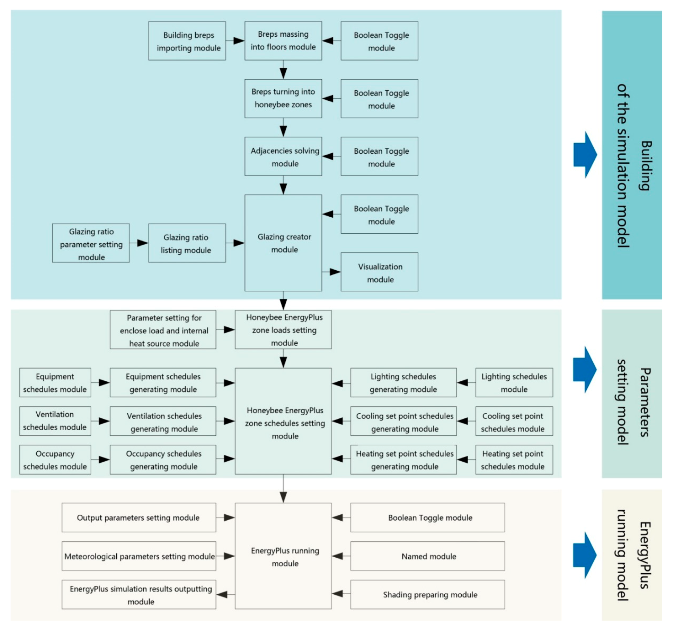
3.3. Physical Model Method (Multi-Zone)

The physical model method is based on the theoretical model and method of the building energy simulation, relying on big data of urban buildings such as the volume, transparency ratio, enclosed structure, occupancy, energy-use system, operation mode, and climate to simulate the urban energy consumption scientifically, accurately, and efficiently. The physical model method uses Grasshopper to search EnergyPlus to simulate the urban energy consumption, as shown in Figure 5. Due to the large number, types, various structures, and complex facilities of urban buildings, it is difficult to simulate energy consumption.

3.3.1. The Components of the Physical Model

The physical model method is a system for simulating urban building energy consumption, which is divided into three parts: building the urban energy consumption model, simulating the urban energy consumption model, and visualizing the urban energy consumption model. The visualization of the urban energy consumption model integrates the simulation results of urban energy consumption into other types of basic information about the city on the GIS platform and presents them as a visual digital map. The components of the simulation module are shown in Figure 6. The following describes the parameter settings in each module: The EnergyPlus running module is used to receive the meteorological files of a typical meteorological year in EPW format, and the schedule module is generated when the connected Boolean setting module inputs the true value, and the honeybee EnergyPlus zone loads setting module is imported into the IDF file. Finally, EnergyPlus runs the IDF file to obtain the CSV result file of the EnergyPlus simulation results.

3.3.2. Parameter Settings of the Physical Model

In this study, the building types in the study area are divided into residential buildings and public buildings. According to the building types, parameters such as the glazing ratio, enclosure load, and internal heat source are set. The specific parameter values are shown in Table 2, Table 3 and Table 4. The equipment generating schedule of residential buildings is shown as number 1 and number 2 in Table 3, and the schedule of public buildings is shown as number 3 and number 4 in Table 3; the decimal value represents the percentage of equipment usage. The ventilation schedule of residential buildings is shown as number 5 and number 6 in Table 3, and the schedule of public buildings is shown as number 7 and number 8 in Table 3. The number 0 indicates that the fresh air exchanger is not on, and 1 indicates that it is on. The occupancy generating schedule of residential buildings is shown as number 9 and number 10 in Table 3, and the schedule of public buildings is shown as number 11 and number 4 in Table 3; the decimal value represents the percentage of staff in the room. The lighting generating schedule of residential buildings is shown as number 12 and number 13 in Table 3, and the schedule of public buildings is shown as number 11 and number 4 in Table 3; the decimal value represents the percentage of lighting usage. The cooling set point schedule of residential buildings is shown as number 1 and number 2 in Table 4, and the schedule of public buildings is shown as number 3 and number 4 in Table 4. The number 26 means that the air conditioner is turned on when the temperature reaches 26 °C. The number 60 means that the air conditioner is turned on when the temperature reaches 60 °C. Because the temperature is usually lower than 60, 60 means that the air conditioner is off. The heating set point schedule of residential buildings is shown as number 5 and number 6 in Table 4, and the schedule of public buildings is shown as number 7 and number 8 in Table 4. The number 20 means that the air conditioner is turned on when the temperature reaches 20 °C. The number −40 means that the air conditioner is turned on when the temperature reaches −40 °C. Because the temperature is usually higher than −40, −40 means that the air conditioner is off.
The multi-zone model is a physical model method. The multi-zone model is used to simulate the building energy consumption in the HSRS area. The default floor height of all buildings is three meters. Based on the height, the whole building is divided into floors, and each floor of the building is set as a single thermal zone for the energy simulation.

3.4. Physical Model Method (Single-Zone)

The single-zone model is also a kind of physical model, in which the simulation system is the same as that for the multi-zone model. The biggest difference between the single-zone model and the multi-zone model is that the single-zone model sets each building as a thermal zone, while the multi-zone model sets each floor of a building as a thermal zone.
In order to improve the calculation speed, the single-zone model removes the module involving breps massing into floors of the multi-zone model. The single-zone model does not divide the building based on its height but sets the whole building as a thermal zone. When setting parameters, such as the transparency ratio, lighting load, and occupant density, the whole building is regarded as a one-story building. The energy consumption of lighting and equipment calculated by the single-zone model is equal to the energy consumption value of one floor in the multi-zone model. However, air conditioning energy consumption is affected by many factors. The air conditioning energy consumption calculated by this method is not directly equal to the air conditioning energy consumption value of one floor in the multi-zone model, but it needs to be multiplied by the correction coefficient. In the visualization part, the difference between multi-zone and single-zone models is that it is necessary to do a simple formula calculation of the urban energy simulation results before integrating them with other basic urban information.
When calculating the building energy consumption in the HSRS area with a single-zone model, the buildings are also divided into residential buildings and public buildings, and each whole building is set as a thermal zone for simulation. The lighting and equipment energy consumption calculated by the single-zone model is taken as the energy consumption of one floor in the multi-zone model; hence, the number of building stories is a significant type of data. Meanwhile, the air conditioning energy consumption calculated by the method needs to be multiplied by the correction coefficient, and the correction coefficient estimated by the simulation result of the HSRS area is 3.6. The equation of each building’s energy consumption is obtained as follows:
y = a1(x1 + x2) + a2x3
In the equation, y is the energy consumption of each building, x1 is the lighting energy consumption, x2 is the equipment energy consumption based on the number of building floors, x3 is the air conditioning energy consumption, a1 is the number of building floors, and a2 is the correction coefficient with a value of 3.6.

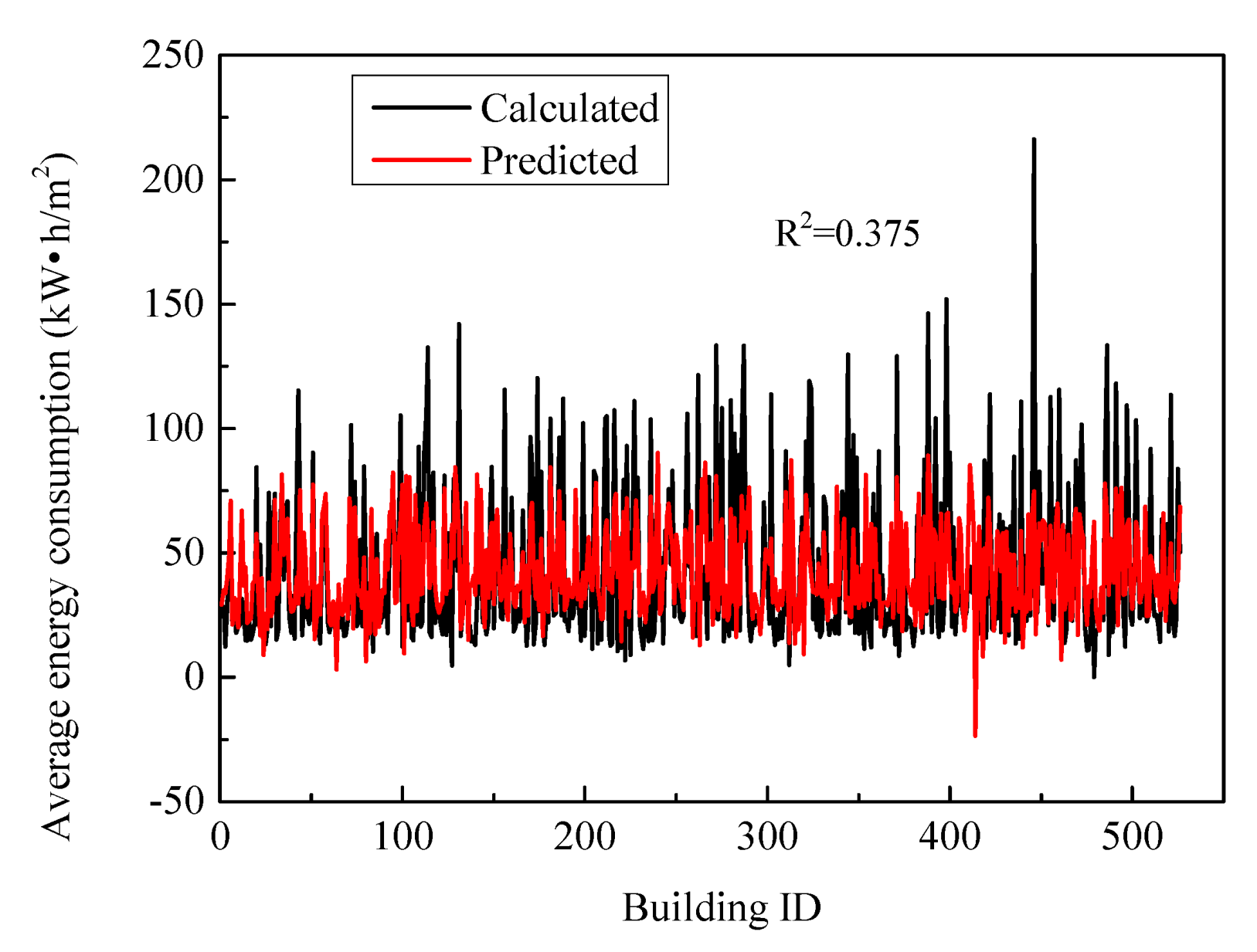
3.5. Data-Driven Model Method (Regression)

The regression method is a kind of data-driven model method. To use the regression method to predict energy consumption, first, the training data need to be prepared. Then, training samples are used to regress the linear equation, and finally, the accuracy of the model is verified.

3.5.1. Urban Energy Consumption Data

This study collected 2628 civil building energy efficiency evaluation data points as training samples, including 1380 residential buildings and 1248 public buildings. The database was compiled from the evaluation report of the theoretical value of civil building energy efficiency of the Jiangsu civil building energy efficiency evaluation institution.

3.5.2. Regression Model for Individual Buildings

This study used the linear regression algorithm in MATLAB to acquire a linear equation. The 2628 civil building energy efficiency evaluation data points were normalized first using the following normalization formula:
x return = | x x m i n | x m a x x m i n
Then, using the linear regression algorithm in MATLAB, the energy consumption per unit area was set as the dependent variable, and other factors were set as independent variables. The linear correlation coefficient and intercept of each independent variable were obtained, and the linear equation of the energy consumption per unit area was obtained as follows:
y = 0.039x1 − 0.388x2 − 0.068x3 + 0.175x4 − 0.087x5 + 0.019x6 − 0.407x7 + 0.404x8 − 0.011x9 + 0.305
In the equation, y is the energy consumption per unit area of each building, x1 is the building area, x2 is the number of building floors, x3 is the eastern window ratio, x4 is the western window ratio, x5 is the southern window ratio, x6 is the northern window ratio, x7 is the shape factor, x8 is the building height, and x9 is the heat transfer coefficient of the window.
In order to ensure the reliability of the training data, 80% of the training data were selected. Finally, the original dataset was divided into 2102 groups for training and 526 groups for testing. The correlation coefficient R2 of the final training data was 0.375, and the comparison between the test value and the predicted value is shown in Figure 7. The results show that there was no strong linear correlation between the nine selected energy consumption factors and energy consumption, so this paper used the neural network for further nonlinear training.

3.5.3. Urban Energy Simulation Using the Regression Model

In this study, the data from the HSRS area were also sorted into two categories: residential and public buildings. The information in the HSRS area dataset also included the energy consumption per unit area, building area, number of floors, window ratio (East, West, South, and North), body shape coefficient, building height, and heat transfer coefficient of the outer window. Then, we put the building dataset of HSRS into Equation (3) to calculate the energy consumption of the HSRS area.

3.6. Data-Driven Model Method (Artificial Neural Network)

The artificial neural network (ANN) method is one kind of data-driven model method. The artificial neural network is a commonly used artificial intelligence algorithm. The process of using artificial intelligence to predict energy consumption is usually divided into four steps, namely data collection, data preprocessing, model training, and model validation.

3.6.1. Urban Energy Consumption Data

For this type of training data, there were also 2628 civil building energy efficiency evaluation data points used in the regression method. The information included the energy consumption per unit area, building area, number of floors, window ratio (East, West, South, and North), body shape coefficient, building height, and the heat transfer coefficient of the outer window. The building energy consumption is the simulated energy consumption calculated by building energy efficiency evaluation software such as EEFC and DeST. The energy consumption and buildings in the database were mostly built after 2010.

3.6.2. Training of the ANN for Individual Energy Consumption

This study also used the BP neural network in MATLAB for programming to train an ANN model to determine the individual building energy consumption. The BP algorithm is the basis of the neural network training algorithm. The 2628 civil building energy efficiency evaluation data points collected were used as a training sample to train a data-driven model. Firstly, the energy efficiency evaluation data collected from 2628 civil buildings were divided into residential buildings and public buildings. The information also included the energy consumption per unit area, the building area, the number of floors, the window ratio (East, West, South, and North), the body shape coefficient, the building height, and the heat transfer coefficient of the outer window. Then, these data were normalized with the normalization processing formula shown in Equation (2). As with the regression method, 80% of the training data were also used when the neural network was used for training. The correlation coefficient R2 of the final training data was 0.632, and the comparison between the test set and the predicted value is shown in Figure 8. The results show that after training with the BP neural network, the correlations between influencing factors and energy consumption became stronger, which shows that neural network can be used as a method of energy consumption prediction.

3.6.3. Urban Energy Simulation Using the ANN

After the training of the ANN for individual building energy consumption, this study used MATLAB for programming to simulate the energy consumption in the HSRS area. The dataset of the HSRS area was input, and the energy consumption per unit area of each building in the HSRS area was calculated.

4. Results and Analysis

In this paper, building energy consumption in HSRS area was simulated using the multi-zone model, single-zone model, regression method, and artificial neural network method. Next, the four methods were compared and analyzed from three aspects: urban energy consumption patterns, dynamic nature, and simulation performance.

4.1. Urban Energy Consumption Patterns

4.1.1. Comparison of the Urban Energy Consumption

This paper compares the results calculated by four different methods, including the annual total energy consumption, the annual total energy consumption of residential buildings, the annual total energy consumption of public buildings, the energy consumption per unit area, the energy consumption per unit area of residential buildings, and the energy consumption per unit area of public buildings. In terms of the annual total energy consumption, the calculated values of the multi-zone and single-zone were the largest, and the calculated values of the linear regression were the smallest; meanwhile, the calculated values of the multi-zone and single-zone were similar, and the calculated values of the linear regression and ANN were similar. The average value was 2.9 × 10⁸ kw·h, and the calculated results for the multi-zone, single-zone, and ANN were closer to the average value. When considering the total annual energy consumption of residential buildings, the calculated value of the single-zone was the largest, and the calculated value of the ANN was the smallest. In addition, the calculated values of the multi-zone and single-zone were similar, and the calculated value of the linear regression was similar to that of the ANN. The average values were similar among the four calculated results. As for the total annual energy consumption of public buildings, the calculation value of the multi-zone was the largest, and the calculation value of the linear regression was the smallest. The calculation results of the multi-zone, single-zone, and ANN were closer to the average value. In view of the energy consumption per unit area, the energy consumption per unit area of residential buildings, and the energy consumption per unit area of public buildings, the calculation value of the single-zone was the largest, and the calculation value of the linear regression and ANN was smaller. The average values were 53.51, 44.95, and 63.31 kw·h/m2, respectively, so the calculation value of the multi-zone was close to the average value (as shown in Table 5).

4.1.2. Comparison of the Urban Energy Consumption

Because public buildings and residential buildings differ in terms of their transparency ratios, schedules, and other parameters, this study divided buildings into residential buildings and public buildings to calculate energy consumption. The following results can be intuitively obtained from Figure 9. Firstly, we compared the calculated results for the energy consumption intensity of the four methods. The average values of the multi-zone and single-zone were large, while the average values of the linear regression and the ANN were small. Secondly, from the median and the space between the upper and lower four digits of each box plot, it can be seen that the distribution of the calculated values of the linear regression was very symmetrical, while the calculated values of other methods were mostly distributed above the average. In addition, the simulation values of the multi-zone and single-zone were scattered, and the linear regression and ANN calculations were more concentrated. Finally, there were extremely few outliers when compared with the public building calculation results of the multi-zone and linear regression methods, while in the calculation results of the residential buildings, the linear regression and ANN had extremely large outliers.

4.2. Dynamic Nature of Energy Consumption

4.2.1. The Analyze of Multi-Zone and Single-Zone Model

The multi-zone model takes into account the influences of the different floors of the building, while the single-zone model regards a building as a thermal zone, which directly led to the difference in air-conditioning energy consumption observed between the two methods. When building energy consumption simulation software is used to directly simulate urban energy consumption, detailed building datasets are needed. The building dataset adopted in this study was modeled to a certain extent, just as an archetype of buildings using the same transparency ratio, the same heat transfer coefficient of the external wall, and the same occupant density. The regression method and artificial neural network method can be used to calculate the annual total energy consumption and unit area energy consumption of each building, but they cannot be used to analyze the monthly, weekly, and hourly energy consumption changes. In urban planning and design, the building scheme changes with the change of the design concept. The multi-zone model and single-zone model can accurately calculate the required energy consumption according to the change in the scheme, which can enable designers to carry out urban design on the basis of low urban energy consumption.
Multi-zone models play an important role in distributed energy, urban energy station, building operation, energy security, real-time monitoring, urban energy management, urban planning and design, urban energy policy and building renovation, etc. The applications of multi-zone models can be summarized into three aspects, including big database, real-time monitoring and building renovation.
  • Big database
The data required for multi-zone models can be divided into three categories: three-dimensional geometric data representing the shape of the buildings, non-geometric data with significant impact on energy consumption, and data controlling the process of urban energy simulation. A large number of buildings should be considered in multi-zone models. The number of simulation parameters involved is tens of thousands, most of which can reach million level. Big databases provide corresponding support not only for the researches of urban energy conservation and urban planning, but also for other disciplines including geography, transportation and social sciences.
  • Real-time monitoring
Multi-zone models provide dynamic energy information with hourly accuracy and realize real-time energy monitoring of each building. Their electricity consumption behavior can be adjusted by users according to the hourly energy consumption. For example, because of the flexible production schedule of iron and steel enterprises, the enterprises can adjust the working time of some production lines to taking advantage of the valley price of the time-of-use electricity pricing system to reduce the cost.
  • Building renovation
The transformation of existing buildings is an effective measure to improve the energy utilization efficiency of buildings, alleviating the greenhouse effect and climate change. City managers should use tools to evaluate and optimize energy-saving measures at city scale in order to design incentives accordingly. Multi-zone models can quickly establish and run the building energy model at urban scale to analyze urban building energy saving strategies. In terms of old city renovation, the energy-saving potential and cost-effectiveness of building energy-saving measures can be evaluated by the results of multi-zone models.
The multi-zone and single-zone models are based on a scientifically mature building energy consumption model that relies on detailed multi-source big data, and, in this study, the simulation results were found to be scientific and accurate. The simulation results of this method were highly correlated with urban space, and the energy consumption could be viewed at different levels and scales.

4.2.2. The Dynamic Nature of the Multi-Zone and Single-Zone Models

The simulation results of the multi-zone and single-zone models could be observed at the hourly level, and the energy consumption change could be presented according to the year, month, day, and hour. The simulation was able to output a variety of energy consumption indicators (extreme, average, total), which can output energy consumption components and could be used for scenario prediction analysis of future urban energy consumption.
Figure 10 shows the monthly, daily, and hourly energy consumption of the HSRS area. The plots of monthly energy consumption show that energy consumption was high in winter and summer, while the energy consumption was low in spring and autumn. As depicted in the pictures of the daily energy consumption changes in January and July, it can be easily seen that the energy consumption of public buildings underwent no energy consumption changes at weekends. In the hourly energy consumption changes on 12 January and 21 July, from 19:00 to 8:00 of the next day, residential buildings consumed energy, and from 20:00 to 23:00, the energy consumption was very high; the public buildings consumed energy from 7:00 to 19:00, and the energy consumption increased first and then decreased. The monthly, daily, and hourly energy consumption changes reflect consistent dynamic trends for the two methods.

4.3. Simulation Performance

The simulation performance of the four methods can be embodied by four aspects, namely the data required, the simulation workflow development, the simulation speed, and the vulnerability to errors.
Firstly, the classification of the data, data components, and data formats of the four methods are different in terms of the requirements of data acquisition. When using the physical model method to calculate urban energy consumption, data acquisition and collation work require a lot of time and resources. In data preparation of the multi-zone model and single-zone model, the building dataset that needs to be acquired is mainly divided into geometric data and non-geometric data. Geometric data mainly include 2D footprint polygons and building heights. Geometric data acquisition generally occurs via two methods: one is to provide data by public institutions, the other is to obtain data through maps. Among them, the comprehensiveness and reliability of the data obtained from maps need to be verified. There are many kinds of non-geometric data that affect the energy consumption of urban buildings, and the acquisition of each kind of data, such as occupant density, is a challenge. Occupant density data can be divided into commercial, official, residential, and other types of building occupant density. The acquisition of measured data regarding the occupant density in each type of building requires a certain amount of time and material resources. In the physical model method, the multi-zone method and single-zone method require the necessary computer technology to process the big data of urban buildings on the GIS platform. Through the use of other suitable software, such as Rhino and Grasshopper, the conversion from GIS data to IDF data can be realized, and then EnergyPlus can be used to process the big data of urban buildings to ensure accuracy and efficiency. The preliminary data used in the regression method and artificial neural network method were data points from the energy efficiency evaluation of 2652 civil buildings. The original format of these data was PDF. In this study, PDF data were converted into TXT files, which made the data into readable text. Then, Visual Studio Code was used for programming. According to different keyword locations, the corresponding data were read and finally written into Excel.
Secondly, the simulation workflow development of the four methods was different. In terms of modeling efficiency, the rhinoceros automatic stretching block program was needed for the modelling of multi-zone and single-zone models, and the ANN and regression model methods also required the use of MATLAB programs. The four methods took almost the same amount of time for the process of coding—about an hour.
Thirdly, from the point of the simulation speed, the buildings in the study area of HSRS were modeled according to the modeling principles of the multi-zone model. The three-dimensional model of the city was simulated by the energy consumption simulation system of urban buildings. In this study, the building block of the HSRS area was divided into eight areas to simulate energy consumption. Each floor of the building was a thermal area. The purpose of the zoning method was to improve the calculation speed. The total calculation time of the HSRS area was about 86.2 h. The calculation time for the single-zone model was 24.2 h. The calculation time for the regression method and neural network method was about 1–1.4 s (as shown in Table 6).
Lastly, there were differences in the vulnerability to errors in the four methods. The above simulation time does not include the time taken to eliminate errors in the simulation process. The multi-zone and single-zone model methods require a high-quality three-dimensional model that must be a closed model. Otherwise, errors will be reported in the simulation process. Geometric models need to be checked after error reporting to identify problems and rebuild models. However, the ANN and regression model methods rarely cause errors when the training data are cleaned well.

4.4. Limitations and Future Research

HSRS project is an urban design in a limited new site in already urbanized area. There are three transformer substations in the research area, and the geographical load radius of each transformer substation is about 2 km. When dealing with similar design cases, the advantage of the multi-zone models is its accuracy, but the limitation is that it is necessary to determine the design strategy according to the specific local conditions in order to create regional synergy energy value. In future studies, it will be advantageous to propose a catchment area with a certain energy factor should not exceed a certain area and certain energy value, making it more sustainable and energy efficient.

5. Conclusions

Through a literature review and discussion, this paper has summarized the top-down and bottom-up approaches of urban energy simulation methods and classified these methods by analyzing their advantages and disadvantages. This paper also compared the differences in data inputs, suitable scales, accuracy, and computing speed with several representative methods in the HSRS area, providing a selective reference for urban designers.
The advantage of a multi-zone model is that it is easy to operate, and it can run on the established urban energy simulation system to complete the urban energy simulation. This method relies on building simulation tools, so the calculation process takes a long time. The biggest challenge is preparing the building dataset of the city, such as the building form, insulation thickness, and transparency ratio. In the case of a detailed building dataset, highly accurate energy consumption data, and sufficient time, the multi-zone model can be used. The advantage of the single-zone model is that it has a high level of accuracy and can simulate buildings of any scale. The difference between the single-zone model and multi-zone model is that the calculation speed is greatly improved on the basis of guaranteeing the correct rate. However, the difficulty of this single-zone model is the same as that of the multi-zone model, which is the acquisition of the building dataset. Compared with the multi-zone model, the single-zone model is more suitable for urban planning projects with certain time constraints. The regression method is fast in terms of calculation, but its accuracy level is low, and the interaction between buildings cannot be considered. The regression method is typically used for calculating urban energy consumption. When detailed and reliable statistical data are available and the energy consumption data has a low level of accuracy, this method can be considered. The advantage of the ANN method is that it can simulate buildings of any scale. The buildings do not need to be optimized before being simulated. It is more economical and can compare the simulated energy consumption results and the measured energy consumption data at the level of each building. The shortcomings of this method are the need for low-scale statistical data, disputes over current statistical data, and the need for continuous statistical data to avoid information errors. The artificial neural network algorithm can achieve or even exceed the accuracy of the single-zone model when the training sample data are perfect. The data-driven model method has a fast calculation speed, so it is worth studying and exploring it to improve its accuracy and integration with urban planning software.
The research on urban energy simulation methods needs to be improved in the hope that a big data platform of urban energy consumption can be established in the future with functions of simulation, measurement, and analysis. The urban energy simulation method has been applied to urban planning and urban design and can also explore the relationship between urban form and other factors related to energy consumption. This area of study could explore the mechanisms related to urban spatial form and energy consumption and assess the sensitivity between energy consumption and urban form factors. Urban energy simulation can be used to determine the energy interactions between individual buildings and blocks. Moreover, it can be used to provide guidelines for the achievement of low-energy-oriented urban design to facilitate urban planners and designers in tackling problems at the early stage of their work. Promoting the collaborative application of the big data related to energy consumption, urban energy simulation could be applied for optimization modeling and energy-driven urban design.

6. Patents

  • Yanxia Li, Xing Shi, Junyan Yang, Xinkai Zhang, Annan Wang. A modeling method of urban building energy consumption model, 2018.
  • Yanxia Li, Binghui Si, Xing Shi, Dian Zhang, Yue Wu. A simulation system for urban buildings’ energy consumption, 2019.

Author Contributions

Conceptualization: Y.L. and X.S.; methodology: Y.L.; software: Y.L.; validation: Y.L., X.Z., S.Z., C.W., and S.W.; investigation: Y.L.; data curation: Y.L.; writing—original draft preparation: Y.L.; writing—review and editing: Y.L., X.Z., S.Z., J.Y., and X.S.; funding acquisition: X.S. All authors have read and agreed to the published version of the manuscript.

Funding

This research was funded by the National Natural Science Foundation of China (grant number 51678124).

Conflicts of Interest

The authors declare no conflict of interest.

References

  1. Wang, S.; Fang, C.; Guan, X.; Pang, B.; Ma, H. Urbanisation, energy consumption, and carbon dioxide emissions in China: A panel data analysis of China’s provinces. Appl. Energy 2014, 136, 738–749. [Google Scholar] [CrossRef]
  2. Van De Wal, R.S.W.; De Boer, B.; Lourens, L.J.; Köhler, P.; Bintanja, R. Reconstruction of a continuous high-resolution CO2 record over the past 20 million years. Clim. Past 2011, 7, 1459–1469. [Google Scholar] [CrossRef]
  3. United Nations. World Urbanization Prospects: 2015 Revision; United Nations, Department of Economics and Social Affairs, Population Division: New York, NY, USA, 2015. [Google Scholar]
  4. United Nations. World Urbanization Prospects: 2014 Revision; United Nations, Department of Economic and Social Affairs, Population Division: New York, NY, USA, 2014. [Google Scholar]
  5. Seto, K.C.; Güneralp, B.; Hutyra, L.R. Global forecasts of urban expansion to 2030 and direct impacts on biodiversity and carbon pools. Proc. Natl. Acad. Sci. USA 2012, 109, 16083–16088. [Google Scholar] [CrossRef] [PubMed]
  6. United Nations. World Urbanization Prospects: The 2009 Revision; United Nations: New York, NY, USA, 2010. [Google Scholar]
  7. UN-Habitat. Energy. 2012. Available online: http://unhabitat.org/urbanthemes/energy/ (accessed on 8 November 2016).
  8. Chambers, A.; Nakicenovic, N. World Energy Outlook 2008; IEA/OECD: Paris, France, 2008. [Google Scholar]
  9. Sovacool, B.K.; Brown, M.A. Twelve metropolitan carbon footprints: A preliminary comparative global assessment. Energy Policy 2010, 38, 4856–4869. [Google Scholar] [CrossRef]
  10. Grübler, A.; Bai, X.; Buettner, T.; Dhakal, S.; Fisk, D.; Ichinose, T.; Keirstead, J.; Sammer, G.; Satterthwaite, D.; Schulz, N.B.; et al. Urban Energy Systems. In Global Energy Assessment (GEA); Cambridge University Press (CUP): Cambridge, UK, 2012; pp. 1307–1400. [Google Scholar] [CrossRef]
  11. UNEP. Cities and Climate Change. 2015. Available online: http://www.unep.org/resourceefficiency/Policy/ResourceEfficientCities/FocusAreas/CitiesandClimateChange/tabid/101665/Default.asp (accessed on 5 June 2016).
  12. Chalal, M.L.; Benachir, M.; White, M.; Shrahily, R. Energy planning and forecasting approaches for supporting physical improvement strategies in the building sector: A review. Renew. Sustain. Energy Rev. 2016, 64, 761–776. [Google Scholar] [CrossRef]
  13. Yang, Z.; Ghahramani, A.; Becerik-Gerber, B. Building occupancy diversity and HVAC (heating, ventilation, and air conditioning) system energy efficiency. Energy 2016, 109, 641–649. [Google Scholar] [CrossRef]
  14. Becker, S.; Frew, B.A.; Andresen, G.B.; Jacobson, M.Z.; Schramm, S.; Greiner, M. Renewable build-up pathways for the US: Generation costs are not system costs. Energy 2015, 81, 437–445. [Google Scholar] [CrossRef]
  15. Comodi, G.; Cioccolanti, L.; Renzi, M. Modelling the Italian household sector at the municipal scale: Micro-CHP, renewables and energy efficiency. Energy 2014, 68, 92–103. [Google Scholar] [CrossRef]
  16. Broin, E.Ó.; Mata, É.; Göransson, A.; Johnsson, F. The effect of improved efficiency on energy savings in EU-27 buildings. Energy 2013, 57, 134–148. [Google Scholar] [CrossRef]
  17. Parshall, L.; Gurney, K.; Hammer, S.A.; Mendoza, D.; Zhou, Y.; Geethakumar, S. Modeling energy consumption and CO2 emissions at the urban scale: Methodological challenges and insights from the United States. Energy Policy 2010, 38, 4765–4782. [Google Scholar] [CrossRef]
  18. Davila, C.C.; Reinhart, C.F.; Bemis, J.L. Modeling Boston: A workflow for the efficient generation and maintenance of urban building energy models from existing geospatial datasets. Energy 2016, 117, 237–250. [Google Scholar] [CrossRef]
  19. Sola, A.; Corchero, C.; Salom, J.; Sanmarti, M. Simulation Tools to Build Urban-Scale Energy Models: A Review. Energies 2018, 11, 3269. [Google Scholar] [CrossRef]
  20. Shi, Z.; Fonseca, J.A.; Schlueter, A. A review of simulation-based urban form generation and optimization for energy-driven urban design. Build. Environ. 2017, 121, 119–129. [Google Scholar] [CrossRef]
  21. Aydinalp, M.; Ugursal, V.I.; Fung, A.S. Modeling of the appliance, lighting, and space-cooling energy consumptions in the residential sector using neural networks. Appl. Energy 2002, 71, 87–110. [Google Scholar] [CrossRef]
  22. U.S. Green Building Council (USGBC). Green Building Design and Construction; U.S. Green Building Council (USGBC): Washington, DC, USA, 2009. [Google Scholar]
  23. Barlow, S. Guide to BREEAM; RIBA Publishing: London, UK, 2011. [Google Scholar]
  24. Green Chinese Building Evaluation Label. Available online: http://www.cngb.org.cn/ (accessed on 24 November 2015).
  25. Shi, X.; Tian, Z.; Chen, W.; Si, B.; Jin, X. A review on building energy efficient design optimization rom the perspective of architects. Renew. Sustain. Energy Rev. 2016, 65, 872–884. [Google Scholar] [CrossRef]
  26. Chen, Y.; Hong, T.; Piette, M.A. City-Scale Building Retrofit Analysis: A Case Study using CityBES. In Proceedings of the 15th IBPSA Conference, San Francisco, CA, USA, 7–9 August 2017; pp. 1084–1091. [Google Scholar]
  27. Tardioli, G.; Kerrigan, R.; Oates, M.; O’Donnell, J.; Finn, D. Data Driven Approaches for Prediction of Building Energy Consumption at Urban Level. Energy Procedia 2015, 78, 3378–3383. [Google Scholar] [CrossRef]
  28. Li, W.; Zhou, Y.; Cetin, K.; Eom, J.; Wang, Y.; Chen, G.; Zhang, X. Modeling urban building energy use: A review of modeling approaches and procedures. Energy 2017, 141, 2445–2457. [Google Scholar] [CrossRef]
  29. Swan, L.G.; Ugursal, V.I. Modeling of end-use energy consumption in the residential sector: A review of modeling techniques. Renew. Sustain. Energy Rev. 2009, 13, 1819–1835. [Google Scholar] [CrossRef]
  30. Kavgic, M.; Mavrogianni, A.; Mumovic, D.; Summerfield, A.; Stevanovic, Z.; Djurovic-Petrovic, M. A review of bottom-up building stock models for energy consumption in the residential sector. Build. Environ. 2010, 45, 1683–1697. [Google Scholar] [CrossRef]
  31. Chen, Y.; Hong, T. Impacts of building geometry modeling methods on the simulation results of urban building energy models. Appl. Energy 2018, 215, 717–735. [Google Scholar] [CrossRef]
  32. Fernandez-Antolin, M.-M.; Del Río, J.M.; González-Lezcano, R. Influence of Solar Reflectance and Renewable Energies on Residential Heating and Cooling Demand in Sustainable Architecture: A Case Study in Different Climate Zones in Spain Considering Their Urban Contexts. Sustainability 2019, 11, 6782. [Google Scholar] [CrossRef]
  33. Nouvel, R.; Zirak, M.; Dastageeri, H.; Coors, V.; Eicker, U. Urban energy analysis based on 3D city model for national scale applications. In Proceedings of the IBPSA Germany Conference, Aachen, Germany, 22–24 September 2014; Volume 8. [Google Scholar]
  34. Bentzen, J.; Engsted, T. A revival of the autoregressive distributed lag model in estimating energy demand relationships. Energy 2001, 26, 45–55. [Google Scholar] [CrossRef]
  35. Zhang, Q. Residential energy consumption in China and its comparison with Japan, Canada, and USA. Energy Build. 2004, 36, 1217–1225. [Google Scholar] [CrossRef]
  36. Fonseca, J.A.; Schlueter, A. Integrated model for characterization of spatiotemporal building energy consumption patterns in neighborhoods and city districts. Appl. Energy 2015, 142, 247–265. [Google Scholar] [CrossRef]
  37. Reinhart, C.; Davila, C.C. Urban building energy modeling—A review of a nascent field. Build. Environ. 2016, 97, 196–202. [Google Scholar] [CrossRef]
  38. Kruger, A.; Kolbe, T.H. Building Analysis for Urban Energy Planning Using Key Indicators on Virtual 3D City Models—The Energy Atlas of Berlin. Proc. ISPRS Congr. 2012, 145–150. [Google Scholar] [CrossRef]
  39. Gröger, G.; Plümer, L. CityGML—Interoperable semantic 3D city models. ISPRS J. Photogramm. Remote Sens. 2012, 71, 12–33. [Google Scholar] [CrossRef]
  40. Papadopoulos, G.; Edwards, P.; Murray, A. Confidence estimation methods for neural networks: A practical comparison. IEEE Trans. Neural Netw. 2001, 12, 1278–1287. [Google Scholar] [CrossRef]
  41. Tu, J.V. Advantages and disadvantages of using artificial neural networks versus logistic regression for predicting medical outcomes. J. Clin. Epidemiol. 1996, 49, 1225–1231. [Google Scholar] [CrossRef]
  42. Parti, M.; Parti, C. The Total and Appliance-Specific Conditional Demand for Electricity in the Household Sector. Bell J. Econ. 1980, 11, 309. [Google Scholar] [CrossRef]
  43. Yilmaz, L.; Chan, W.K.V.; Moon, I.; Roeder, T.M.K.; Macal, C.; Rossetti, M.D. A review of artificial intelligence based building energy prediction with a focus on ensemble prediction models. In Proceedings of the 2015 Winter Simulation Conference, Huntington Beach, CA, USA, 6–9 December 2015. [Google Scholar]
  44. Zhao, H.-X.; Magoulès, F. A review on the prediction of building energy consumption. Renew. Sustain. Energy Rev. 2012, 16, 3586–3592. [Google Scholar] [CrossRef]
  45. Koksal, M.A.; Ugursal, V.I. Comparison of neural network, conditional demand analysis, and engineering approaches for modeling end-use energy consumption in the residential sector. Appl. Energy 2008, 85, 271–296. [Google Scholar] [CrossRef]
  46. Kalogirou, S.A. Artificial neural networks in energy applications in buildings. Int. J. Low-Carbon Technol. 2006, 1, 201–216. [Google Scholar] [CrossRef]
  47. Caputo, P.; Costa, G.; Ferrari, S. A supporting method for defining energy strategies in the building sector at urban scale. Energy Policy 2013, 55, 261–270. [Google Scholar] [CrossRef]
  48. Ascione, F.; De Masi, R.F.; Rossi, F.D.; Fistola, R.; Sasso, M.; Vanoli, G.P. Analysis and diagnosis of the energy performance of buildings and districts: Methodology, validation and development of Urban Energy Maps. Cities 2013, 35, 270–283. [Google Scholar] [CrossRef]
  49. Ascione, F.; Canelli, M.; De Masi, R.F.; Sasso, M.; Vanoli, G.P. Combined cooling, heating and power for small urban districts: An Italian case-study. Appl. Therm. Eng. 2014, 71, 705–713. [Google Scholar] [CrossRef]
  50. Taylor, S.C.; Fan, D.; Rylatt, R.M. Enabling urban-scale energy modelling: A new spatial approach. Build. Res. Inf. 2013, 42, 4–16. [Google Scholar] [CrossRef]
  51. Mastrucci, A.; Baume, O.; Stazi, F.; Leopold, U. Estimating energy savings for the residential building stock of an entire city: A GIS-based statistical downscaling approach applied to Rotterdam. Energy Build. 2014, 75, 358–367. [Google Scholar] [CrossRef]
  52. Jones, P.; Patterson, J.; Lannon, S. Modelling the built environment at an urban scale—Energy and health impacts in relation to housing. Landsc. Urban Plan. 2007, 83, 39–49. [Google Scholar] [CrossRef]
  53. Orehounig, K.; Mavromatidis, G.; Evins, R.; Dorer, V.; Carmeliet, J. Towards an energy sustainable community: An energy system analysis for a village in Switzerland. Energy Build. 2014, 84, 277–286. [Google Scholar] [CrossRef]
  54. Kaempf, J.; Robinson, D. A simplified thermal model to support analysis of urban resource flows. Energy Build. 2007, 39, 445–453. [Google Scholar] [CrossRef]
  55. Robinson, D.H.; Kämpf, J.; Leroux, P.; Perez, D.; Rasheed, A.; Wilke, U. CITYSIM: Comprehensive micro-simulation of resource flows for sustainable urban planning. In Proceedings of the Eleventh International IBPSA Conference, Glasgow, UK, 27–30 July 2009. [Google Scholar]
  56. Nielsen, H.A.; Madsen, H. Modelling the heat consumption in district heating systems using a grey-box approach. Energy Build. 2006, 38, 63–71. [Google Scholar] [CrossRef]
  57. Lauster, M.; Teichmann, J.; Fuchs, M.; Streblow, R.; Mueller, D. Low order thermal network models for dynamic simulations of buildings on city district scale. Build. Environ. 2014, 73, 223–231. [Google Scholar] [CrossRef]
  58. Kim, E.-J.; Plessis, G.; Hubert, J.-L.; Roux, J.-J. Urban energy simulation: Simplification and reduction of building envelope models. Energy Build. 2014, 84, 193–202. [Google Scholar] [CrossRef]
  59. Swan, L.; Ugursal, V.I.; Beausoleil-Morrison, I. Implementation of a Canadian residential energy end-use model for assessing new technology impact. In Proceedings of the Eleventh International IBPSA Conference, Glasgow, UK, 27–30 July 2009. [Google Scholar]
  60. Mohmed, A.; Ugursal, V.I.; Beausoleil-Morrison, I. A new methodology to predict the GHG emission reductions due to electricity savings in the residential sector. In Proceedings of the Third Canadian Solar Buildings Conference, Fredericton, NB, Canada, 20–22 August 2008. [Google Scholar]
  61. Aydinalp, M.; Ugursal, V.I.; Fung, A.S. Modeling of the space and domestic hot-water heating energy-consumption in the residential sector using neural networks. Appl. Energy 2004, 79, 159–178. [Google Scholar] [CrossRef]
  62. Znouda, E.; Ghrab-Morcos, N.; Hadj-Alouane, A. Optimization of Mediterranean building design using genetic algorithms. Energy Build. 2007, 39, 148–153. [Google Scholar] [CrossRef]
  63. Tuhus-Dubrow, D.; Krarti, M. Genetic-algorithm based approach to optimize building envelope design for residential buildings. Build. Environ. 2010, 45, 1574–1581. [Google Scholar] [CrossRef]
  64. Foucquier, A.; Robert, S.; Suard, F.; Stephan, L.; Jay, A. State of the art in building modelling and energy performances prediction: A review. Renew. Sustain. Energy Rev. 2013, 23, 272–288. [Google Scholar] [CrossRef]
Figure 1. Classification of urban energy simulation methodology.
Energies 13 04781 g001
Figure 2. Location of the research area.
Energies 13 04781 g002
Figure 3. Functional area of Hangzhou South Station.
Energies 13 04781 g003
Figure 4. Plane and elevation modeling principles of the urban energy consumption model: (a) plane before modeling and after modeling; (b) elevation before modeling and after modeling.
Energies 13 04781 g004
Figure 5. Physical model method workflow.
Energies 13 04781 g005
Figure 6. Components of the urban building energy simulation.
Energies 13 04781 g006
Figure 7. Comparisons of the multi-zone method and single-zone method.
Energies 13 04781 g007
Figure 8. Comparisons of the multi-zone method and single-zone method.
Energies 13 04781 g008
Figure 9. Comparison of energy consumption per unit area of four calculation methods: (a) dispersion of energy consumption intensity of public buildings; (b) dispersion of energy consumption intensity of residential buildings.
Energies 13 04781 g009
Figure 10. Energy consumption of residential and public buildings (MWh/m2·a): (a) monthly energy consumption of residential buildings; (b) monthly energy consumption of public buildings; (c) daily energy consumption of residential buildings in January; (d) daily energy consumption of public buildings in January; (e) daily energy consumption of residential buildings in July; (f) daily energy consumption of public buildings in July; (g) hourly energy consumption of residential buildings on 12 January; (h) hourly energy consumption of public buildings on 12 January; (i) hourly energy consumption of residential buildings on 21 July; (j) hourly energy consumption of public buildings on 21 July.
Energies 13 04781 g010
Table 1. Characteristics of bottom-up approaches.
MethodsData-Driven Model MethodHybrid Model MethodPhysical Model Method (Simplified)Physical Model Method (Archetype)Physical Model Method (Detailed)
Advantages• Accurate prediction
• Statistical regression method
• Fast processing speed
• Small simulation load
• Small workload
• Fast processing speed
• Moderate workload
• Fast calculation speed
• Good accuracy at a large scale
• High accuracy and good universality
• Suitable for macro, meso, and micro scale
Limitations• Limited scalability
• Difficult to integrate with urban forms
• Limited scalability
• General accuracy
• General precision
• Building parameters ignorance
• Ignorance of the heterogeneity of same buildings
• Insufficient accuracy
• Large workload
• Slow calculation speed
• High data requirements
Table 2. EnergyPlus Parameter Settings.
Building TypeGlazing RatioLighting LoadEquipment LoadOccupant DensityAir InfiltrationFresh Air Volume
EastSouthWestNorth
Residential buildings0.170.220.070.197 w/m24.3 w/m20.05 people/m20.00025 m3/s−1·m−2/
Public buildings0.170.30.070.2510 w/m27.64 w/m20.325 people/m20.00021 m3/s−1·m−20.0002 m3/s−1·m−2
Table 3. The equipment schedule.
Schedule Number Hours
01234567891011121314151617181920212223
10.500000000000000000011110.5
2 *0.5000000000.30.30.30.30.30.30.30.30.30.30.31110.5
30.000.000.000.000.000.000.100.500.950.950.950.500.500.950.950.950.950.300.300.000.000.000.000.00
4 *0.000.000.000.000.000.000.000.000.000.000.000.000.000.000.000.000.000.000.000.000.000.000.000.00
5000000000000000000000000
6 *000000000000000000000000
7000000111111111111100000
8 *000000000000000000000000
91.01.01.01.01.01.01.01.01.00.00.00.00.00.00.00.00.00.00.00.51.01.01.01.0
10 *1.01.01.01.01.01.01.01.01.00.50.50.50.50.50.50.50.50.50.50.51.01.01.01.0
110.000.000.000.000.000.000.100.500.950.950.950.800.800.950.950.950.950.300.300.000.000.000.000.00
1200000000000000000000.50.50.50.50
13 *00000000000000000000.50.50.50.50
Without *: Schedule on workday; With *: Schedule at weekend.
Table 4. Temperature control points of the air conditioner.
Schedule NumberHours
01234567891011121314151617181920212223
1262626262626262660606060606060606060606026262626
2 *262626262626262626262626262626262626262626262626
3606060606060606026262626262626262626266060606060
4 *606060606060606060606060606060606060606060606060
52020202020202020−40−40−40−40−40−40−40−40−40−40202020202020
6 *202020202020202020202020202020202020202020202020
7−40−40−40−40−40−40−40−402020202020202020202020−40−40−40−40−40
8 *−40−40−40−40−40−40−40−40−40−40−40−40−40−40−40−40−40−40−40−40−40−40−40−40
Without *: Schedule on workday; With *: Schedule at weekend.
Table 5. The indicators of energy consumption.
IndicatorsMulti-ZoneSingle-ZoneLinear RegressionANNAverage Value
Total annual energy consumption (kW·h)3.3 × 1083.3 × 1082.3 × 1082.6 × 1082.9 × 108
Total annual residential energy consumption (kW·h)8.0 × 1078.5 × 1076.9 × 1076.3 × 1077.4 × 107
Total annual energy consumption of public buildings (kW·h)2.5 × 1082.4 × 1081.6 × 1082.0 × 1082.1 × 108
Energy consumption per unit area (kW·h/m2)60.7271.3440.8641.1153.51
Energy consumption per unit area of residential buildings (kW·h/m2)50.2854.4239.9035.2044.95
Energy consumption per unit area of public buildings (kW·h/m2)72.6690.7041.9647.9063.31
Table 6. Comparison of simulation performance of urban energy consumption simulation methods.
Urban Energy Simulation MethodData RequiredSimulation Workflow DevelopmentIntervention ScaleSimulation Speed (s)
The multi-zone modelGeometric data (2D footprint polygons, building heights), non-geometric data (weather documents, occupant density, transparency ratio, etc.).GIS, Rhino, Grasshopper, EnergyPlusmicro, meso, macro310,320
The single-zone model2 D footprint polygons, building heights, weather documents, occupant density, transparency ratio, etc.GIS, Rhino, Grasshopper, EnergyPlusmicro, meso, macro87,120
The regression methodBuilding type, building area, construction age, heat transfer coefficient of windows, etc. Measured dataAdobe Acrobat Pro, Visual Studio Code Excel, Matlabmeso, macro1–1.4
The artificial neural network methodBuilding type, building area, construction age, heat transfer coefficient of windows, etc. Measured dataAdobe Acrobat Pro, Visual Studio Code, Excel, Matlabmeso, macro1–1.4

