Fault-Structure-Based Active Fault Diagnosis: A Geometric Observer Approach

Abstract

Fault diagnosis techniques can be classified into passive and active types. Passive approaches only utilize the original input and output signals of the system. Because of the small amplitudes, the characteristics of incipient faults are not fully represented in the data of the system, so it is difficult to detect incipient faults by passive fault diagnosis techniques. In contrast, active methods can design auxiliary signals for specific faults and inject them into the system to improve fault diagnosis performance. Therefore, active fault diagnosis techniques are utilized in this article to detect and isolate incipient faults based on the fault structure. A new framework based on observer approach for active fault diagnosis is proposed and the geometric approach based fault diagnosis observer is introduced to active fault diagnosis for the first time. Based on the dynamic equations of residuals, auxiliary signals are designed to enhance the diagnosis performance for incipient faults that have specific structures. In addition, the requirements that auxiliary signals need to meet are discussed. The proposed method can realize the seamless combination of active fault diagnosis and passive fault diagnosis. Finally, a numerical example is presented to demonstrate the effectiveness of the proposed approach, and it is indicated that the proposed method significantly improves the accuracy of the diagnosis for incipient faults.

1. Introduction

With the progress of science and technology, modern industrial systems have become more and more complex, and that leads to higher security risks. Many serious faults are evolved from incipient faults. If faults can be detected as early as possible, measures can be taken to avoid the propagation of faults and avoid the occurrence of vicious accidents, and huge economic and social benefits will be produced. Fault diagnosis techniques, which can judge whether a fault occurs and identify the type and size of the fault, are important means to improve system safety and reliability [1,2,3,4]. In the past few decades, extensive research on fault diagnosis techniques has been made and a series of research results has been published in this area [5,6,7,8,9].

Fault diagnosis techniques can be divided into passive and active types [10]. Passive fault diagnosis (PFD) approaches only utilize the original input and output signals of the system, and, when the fault characteristics are not fully represented in the data, the diagnosis performance is not good. For example, due to the existence of system noise or uncertainty, system changes caused by incipient faults with small amplitudes are indistinguishable from system changes caused by system noise or uncertainty. In addition, the feedback controller in closed-loop system will cover up or compensate the system abnormality caused by fault to a certain extent, which will lead to the poor performance of passive fault diagnosis. In contrast to PFD, active fault diagnosis (AFD) will actively design auxiliary signals according to the fault modes and inject them into systems to excite fault characteristics and improve diagnostic performance [1]. Therefore, active fault diagnosis techniques are utilized in this article to detect and isolate incipient faults.

According to the author’s knowledge, active fault diagnosis framework was first proposed by Zhang et al. [11] in 1988. Subsequently, some scholars carried out research on active fault diagnosis techniques and achieved some results [12]. The Youla–Jabr–Bongiorno–Kucera (YJBK) parameter was employed to build the AFD for incipient faults in [13]. Marseglia et al. [14] considered the design of an input signal required to detect and isolate faults by solving a Mixed Integer Quadratic Program (MIQP). Lin et al. [15] studied active online diagnosis in discrete event systems. Nikoukhah et al. [16] proposed a method to design an auxiliary signal for active failure detection in uncertain linear systems based on the assumption that system noise is bounded. Wang et al. [17] assumed that the disturbance is bounded and proposed an active mechanism to detect multiple modes of operation. Heirung et al. [18] employed the Kolmogorov metric to distinguish a set of system models subject to stochastic disturbances. Blackmore et al. [19] developed an active estimation method for jump Markov linear systems.

As far as the author knows, the number of research results on the application of observer method in active fault diagnosis is limited. Only a few results have been published. Yang et al. [20] designed appropriate auxiliary signals to make the residuals more sensitive to faults and improve the performance of fault diagnosis. Blanchini et al. [21] combined the residual generator with the set-based active fault diagnosis method. By designing a proper residual generator, the residuals generated by different models were restricted to different sets. Scott et al. [22] utilized zonotopes to characterize the set of inputs that were used for active fault diagnosis, and an observer-based method was given for reducing the complexity of this program. Based on zonotopes, a new class of sets called constrained zonotopes was introduced to contain interest sets for estimation and control [23]. Using constrained zonotopes, Raimondo et al. [24] proposed a set-valued observer to achieve rigorous closed-loop active fault diagnosis in a moving horizon framework. The observer method is widely used in passive fault diagnosis, and it is a possible way to realize the combination of active fault diagnosis and passive fault diagnosis. This is another motivation of our work and we want to discuss the application of an observer method in active fault diagnosis.

There are many kinds of observers that can be used for system fault diagnosis, such as Luenberger observer, sliding mode observer, geometric observer, and some hybrid algorithms [25,26]. The geometric observer, which is proposed by Massoumnia et al. [27], has the characteristic that the observer output is only affected by one fault and is robust to all other faults. This feature makes it perform fault detection and fault isolation simultaneously. Thanks to its excellent properties, the geometric observer has been generalized to solve the fault detection and isolation problems for many systems, such as bilinear systems, Markov jump systems, periodic systems, linear parameter-varying systems, and so on [28,29,30,31]. However, to the best of the author’s knowledge, there have been no results of introducing it into active fault diagnosis.

In this paper, the fault diagnosis observer based on a geometric approach is introduced into active fault diagnosis for linear systems for the first time and the contributions of this paper can be summarized as follows:

• A new framework of the fault-structure-based active fault diagnosis is proposed, and the geometric observer is introduced to active fault diagnosis. Using the geometric observer, active fault detection and isolation can be realized simultaneously.
• The requirements of the auxiliary signals are given, and the corresponding auxiliary signals are designed to detect incipient faults. The amplitudes of the designed auxiliary signals are very small and therefore they have little effect on the system performance.
• This proposed method can realize the combination of active fault diagnosis and passive fault diagnosis. For incipient faults, auxiliary signals are designed to carry out active fault diagnosis. For significant faults, passive fault diagnosis can be directly carried out without modifying the observer.

The rest of the paper is outlined as follows. The framework of fault-structure-based active fault diagnosis using geometric observer is proposed in Section 2. In Section 3.1, the design process of fault diagnosis observer based on geometric approach is detailed. According to the dynamic equation of residual, the appropriate auxiliary signals are designed in Section 3.2 and the corresponding evaluation functions are given in Section 3.3. The effectiveness of the proposed approach is verified through numerical simulations in Section 4. Finally, this paper is concluded with some conclusions.

2. Problem Formulation

In this section, the AFD problem for the linear time-invariant (LTI) systems based on fault structure is defined. The framework of the approach is shown in Figure 1, assuming that the system is in operation and there are original inputs $u_k$. As can be seen, observer methods are introduced into active fault diagnosis and a set of special auxiliary signals $a_k$ are designed to assist in the diagnosis of faults with specific structures. The designed auxiliary signals can enhance the performance of faults in the residuals and improve the diagnosis performance for incipient faults. According to the classification of auxiliary signals in [1], the designed auxiliary signals are system-friendly. It is worth noting that the observer only uses the original input of the system (the set input in the open-loop system or the input calculated from the controller in the closed-loop system) and the system output data, and does not directly use the designed auxiliary signals.

Consider the following $n_m$ linear time-invariant systems:

$$\begin{array}{cc}\hfill x_{k+1}& =A^{\left[i\right]}{x}_k+B^{\left[i\right]}{u}_k+B_a^{\left[i\right]}{a}_k^{\left[i\right]}+B_d^{\left[i\right]}{d}_k\hfill \\ \hfill y_k& =C^{\left[i\right]}{x}_k+D_d^{\left[i\right]}{d}_k\hfill \end{array}$$

(1)

where $x_k\in \mathcal{X}$ is the state of the system with dimension $n_x$, $y_k\in \mathcal{Y}$ is the output of the system with dimension $n_y$, $u_k\in \mathcal{U}$ is the input of the system with dimension $n_u$, and $d_k$ denotes the unknown disturbance with bounded power or energy. In particular, $a_k^{\left[i\right]}$ is the designed auxiliary signal for fault mode i. The output matrices $C^{\left[i\right]}$ are right invertible, and system matrices $A^{\left[i\right]},B^{\left[i\right]},C^{\left[i\right]},B_a^{\left[i\right]},B_d^{\left[i\right]},D_d^{\left[i\right]}$ are known constant matrices with appropriate dimensions. The index $i\in I=\{0,1,\dots ,n_m-1\}$ represents the i-th model. Let $i=0$ represent the nominal model without fault and the rests represent different fault modes. In addition, the following assumptions are given.

Assumption 1.

This paper only considers the system parameter faults and actuator faults that are represented by $A^{\left[i\right]}$ and $B^{\left[i\right]}$ respectively. Thus, it is hypothesized that $C^{\left[0\right]}=C^{\left[1\right]}=\cdots =C^{[n_m-1]}$, $B_d^{\left[0\right]}=B_d^{\left[1\right]}=\cdots =B_d^{[n_m-1]}$ and $D_d^{\left[0\right]}=D_d^{\left[1\right]}=\cdots =D_d^{[n_m-1]}$.

Assumption 2.

The auxiliary signal is injected into the input directly, the matrix $B_a^{\left[i\right]}$ is the same as $B^{\left[i\right]}$.

Assumption 3.

Assume that each fault model represents only one fault mode and the fault is time-invariant.

In view of the two different fault types, the processing procedures are given as follows.

Case I: Suppose that the system parameter fault causes the system matrix to change from $A^{\left[0\right]}$ to $A^{\left[i\right]}$. According to Assumption 3, we have $B^{\left[i\right]}=B^{\left[0\right]}$ in this case. Defining ${\widehat{A}}^{\left[i\right]}:=A^{\left[i\right]}-A^{\left[0\right]}$, it is easy that

$$\begin{array}{cc}\hfill x_{k+1}& =(A^{\left[0\right]}+{\widehat{A}}^{\left[i\right]})x_k+B^{\left[i\right]}{u}_k+B_a^{\left[i\right]}{a}_k^{\left[i\right]}+B_d^{\left[i\right]}{d}_k\hfill \\ \hfill & =A^{\left[0\right]}{x}_k+B^{\left[0\right]}{u}_k+B_a^{\left[i\right]}{a}_k^{\left[i\right]}+B_d^{\left[0\right]}{d}_k+{\widehat{A}}^{\left[i\right]}{x}_k\hfill \end{array}$$

(2)

It is assumed that the fault only affects a certain column of matrix $A^{\left[0\right]}$, not the entire matrix. In other words, ${\widehat{A}}^{\left[i\right]}{x}_k$ can be expressed as $L^{\left[i\right]}{m}_k^{\left[i\right]}$, where $L^{\left[i\right]}$ is a column vector used to represent the fault signature and $m_k^{\left[i\right]}$ indicates the fault signal that related to state $x_k$.

Case II: In the case of actuator fault, system input matrix changes from $B^{\left[0\right]}$ to $B^{\left[i\right]}$. Define ${\widehat{B}}^{\left[i\right]}:=B^{\left[i\right]}-B^{\left[0\right]}$. Similar to Case I, we have $A^{\left[i\right]}=A^{\left[0\right]}$ and

$$\begin{array}{cc}\hfill x_{k+1}& =A^{\left[i\right]}{x}_k+(B^{\left[0\right]}+{\widehat{B}}^{\left[i\right]})u_k+B_a^{\left[i\right]}{a}_k^{\left[i\right]}+B_d^{\left[i\right]}{d}_k\hfill \\ \hfill & =A^{\left[0\right]}{x}_k+B^{\left[0\right]}{u}_k+B_a^{\left[i\right]}{a}_k^{\left[i\right]}+B_d^{\left[0\right]}{d}_k+{\widehat{B}}^{\left[i\right]}{u}_k\hfill \end{array}$$

(3)

According to the hypothesis, ${\widehat{B}}^{\left[i\right]}{u}_k$ can also be rewritten as $L^{\left[i\right]}{m}_k^{\left[i\right]}$, where $L^{\left[i\right]}$ is also a column vector used to represent the fault signature and $m_k^{\left[i\right]}$ indicates the fault signal that related to input $u_k$.

Combining the above two cases, the i-th, $i=1,\dots ,n_m-1$ fault model can be reconstructed as

$$\begin{array}{cc}\hfill x_{k+1}& =A^{\left[0\right]}{x}_k+B^{\left[0\right]}{u}_k+L^{\left[i\right]}{m}_k^{\left[i\right]}+B_a^{\left[i\right]}{a}_k^{\left[i\right]}+B_d^{\left[0\right]}{d}_k\hfill \\ \hfill y_k& =C^{\left[0\right]}{x}_k+D_d^{\left[0\right]}{d}_k\hfill \end{array}$$

(4)

For $i=0$, let $L^{\left[0\right]}={\mathbf{0}}^{n_x\times 1}$.

It is time for us to put forward the problem of fault-structure-based active fault diagnosis for LTI systems. For each fault mode i, an observer and an auxiliary signal $a_k^{\left[i\right]}$ are designed to enhance the performance of the fault $L^{\left[i\right]}{m}_k^{\left[i\right]}$ in the observer output, and then carry out fault detection and isolation. The observer and auxiliary signal are designed according to the fault structure $L^{\left[i\right]}$.

3. Main Results

In this section, the proposed method is introduced in detail.

3.1. Geometric Observer Design

In this paper, the geometric observer proposed by Massoumnia in [27] is adopted as the structure-enhanced observer. For fault mode i, the observer is designed as follows:

$$\begin{array}{cc}\hfill z_{k+1}^{\left[i\right]}& =F^{\left[i\right]}{z}_k^{\left[i\right]}-E^{\left[i\right]}{y}_k+G^{\left[i\right]}{u}_k\hfill \\ \hfill r_k^{\left[i\right]}& =M^{\left[i\right]}{z}_k^{\left[i\right]}-H^{\left[i\right]}{y}_k\hfill \end{array}$$

(5)

where $z_k^{\left[i\right]}$ is the observer state and $r_k^{\left[i\right]}$ is the observer output serving as residual signal. $F^{\left[i\right]}$, $E^{\left[i\right]}$, $G^{\left[i\right]}$, $M^{\left[i\right]}$, and $H^{\left[i\right]}$ are observer parameters that need to be designed. It is worth noting that the observer only uses the original input $u_k$ and the system output data $y_k$, and does not directly use the designed auxiliary signal $a_k^{\left[i\right]}$. For the purpose of fault isolation, it is expected that the residual $r_k^{\left[i\right]}$ is only affected by fault mode i and the corresponding auxiliary signal, but not by other fault modes. That is to say,

$$\begin{array}{cc}\hfill m_k^{\left[i\right]}& \mapsto r_k^{\left[i\right]}\mathrm{is}\mathrm{input}\mathrm{observable}\hfill \\ \hfill m_k^{\left[j\right]}& \mapsto r_k^{\left[i\right]}=0,\forall j\ne i\hfill \end{array}$$

(6)

On the observers that satisfy condition (6), we have the following lemma.

Lemma 1.

A set of structure-enhanced observers (5) that satisfy condition (6) exists if

$${\mathcal{L}}^{\left[i\right]}\cap {\mathcal{S}}^{\left[i\right]\ast }=0,i\in \{1,\dots ,n_m-1\}$$

(7)

where ${\mathcal{L}}^{\left[i\right]}=\mathrm{span}\left(L^{\left[i\right]}\right)$ is the range of $L^{\left[i\right]}$ and ${\mathcal{S}}^{\left[i\right]\ast }=inf\underline{\mathcal{S}}\left({\sum }_{j\ne i}{\mathcal{L}}^{\left[j\right]}\right)$. $\underline{\mathcal{S}}\left(\mathcal{L}\right)$ denotes the group of all $(C,A)$-unobservability subspaces containing $\mathcal{L}$, and for the concept of $(C,A)$-unobservability subspaces, please refer to [27].

Proof of Lemma 1. 

This lemma can be directly generalized from theorem 4 in reference [27], and the proof is omitted here. □

Using the geometric method, the observer parameter matrices can be calculated according to the following steps:

• For fault mode i, calculate the unobservability subspaces ${\mathcal{S}}^{\left[i\right]\ast }$;
• Find matrix $D_0^{\left[i\right]}$ satisfying $(A^{\left[0\right]}+D_0^{\left[i\right]}{C}^{\left[0\right]}){\mathcal{S}}^{\left[i\right]\ast }\subset {\mathcal{S}}^{\left[i\right]\ast }$;
• Calculate the canonical projection $P^{\left[i\right]}:\mathcal{X}\to \mathcal{X}/{\mathcal{S}}^{\left[i\right]\ast }$;
• Let $A_0^{\left[i\right]}$ denote the map induced by $A^{\left[0\right]}+D_0^{\left[i\right]}{C}^{\left[0\right]}$ on the factor space $\mathcal{X}/{\mathcal{S}}^{\left[i\right]\ast }$;
• Calculate matrix $H^{\left[i\right]}$ satisfying $ker{H}^{\left[i\right]}{C}^{\left[0\right]}={\mathcal{S}}^{\left[i\right]\ast }+ker{C}^{\left[0\right]}$;
• According to the equation $M^{\left[i\right]}{P}^{\left[i\right]}=H^{\left[i\right]}{C}^{\left[0\right]}$, we get $M^{\left[i\right]}$;
• Let $F^{\left[i\right]}=A_0^{\left[i\right]}+D_1^{\left[i\right]}{M}^{\left[i\right]}$. By designing appropriate $D_1^{\left[i\right]}$, the spectrum of $F^{\left[i\right]}$ can be configured, or disturbance suppression can be performed;
• Let $E^{\left[i\right]}=P^{\left[i\right]}{D}_0^{\left[i\right]}+D_1^{\left[i\right]}{H}^{\left[i\right]}$ and $G^{\left[i\right]}=P^{\left[i\right]}{B}^{\left[0\right]}$.

At this point, all parameter matrices of the observer have been obtained. Define $e_k^{\left[i\right]}=z_k^{\left[i\right]}-P^{\left[i\right]}{x}_k$, then it follows that

$$\begin{array}{cc}\hfill e_{k+1}^{\left[i\right]}=& F^{\left[i\right]}{z}_k^{\left[i\right]}-E^{\left[i\right]}{y}_k+G^{\left[i\right]}{u}_k-P^{\left[i\right]}\left(A^{\left[0\right]}{x}_k+B^{\left[0\right]}{u}_k+L^{\left[i\right]}{m}_k^{\left[i\right]}+B_a^{\left[i\right]}{a}_k^{\left[i\right]}+B_d^{\left[0\right]}{d}_k\right)\hfill \\ \hfill =& F^{\left[i\right]}{z}_k^{\left[i\right]}-\left(P^{\left[i\right]}{D}_0^{\left[i\right]}+D_1^{\left[i\right]}{H}^{\left[i\right]}\right)\left(C^{\left[0\right]}{x}_k+D_d^{\left[0\right]}{d}_k\right)-P^{\left[i\right]}{A}^{\left[0\right]}{x}_k-P^{\left[i\right]}{L}^{\left[i\right]}{m}_k^{\left[i\right]}\hfill \\ \hfill & -P^{\left[i\right]}{B}_a^{\left[i\right]}{a}_k^{\left[i\right]}-P^{\left[i\right]}{B}_d^{\left[0\right]}{d}_k\hfill \\ \hfill =& F^{\left[i\right]}{z}_k^{\left[i\right]}-A_0^{\left[i\right]}{P}^{\left[i\right]}{x}_k-D_1^{\left[i\right]}{M}^{\left[i\right]}{P}^{\left[i\right]}{x}_k-\left(P^{\left[i\right]}{D}_0^{\left[i\right]}{D}_d^{\left[0\right]}+D_1^{\left[i\right]}{H}^{\left[i\right]}{D}_d^{\left[0\right]}+P^{\left[i\right]}{B}_d^{\left[0\right]}\right)d_k\hfill \\ \hfill & -P^{\left[i\right]}{L}^{\left[i\right]}{m}_k^{\left[i\right]}-P^{\left[i\right]}{B}_a^{\left[i\right]}{a}_k^{\left[i\right]}\hfill \\ \hfill =& F^{\left[i\right]}{e}_k^{\left[i\right]}-\left(P^{\left[i\right]}{D}_0^{\left[i\right]}{D}_d^{\left[0\right]}+D_1^{\left[i\right]}{H}^{\left[i\right]}{D}_d^{\left[0\right]}+P^{\left[i\right]}{B}_d^{\left[0\right]}\right)d_k-P^{\left[i\right]}\left(L^{\left[i\right]}{m}_k^{\left[i\right]}+B_a^{\left[i\right]}{a}_k^{\left[i\right]}\right)\hfill \\ \hfill r_k^{\left[i\right]}=& M^{\left[i\right]}{z}_k^{\left[i\right]}-H^{\left[i\right]}\left(C^{\left[0\right]}{x}_k+D_d^{\left[0\right]}{d}_k\right)\hfill \\ \hfill =& M^{\left[i\right]}{z}_k^{\left[i\right]}-M^{\left[i\right]}{P}^{\left[i\right]}{x}_k-H^{\left[i\right]}{D}_d^{\left[0\right]}{d}_k\hfill \\ \hfill =& M^{\left[i\right]}{e}_k^{\left[i\right]}-H^{\left[i\right]}{D}_d^{\left[0\right]}{d}_k\hfill \end{array}$$

(8)

Remark 1.

According to lemma 1 and the design steps of the observer, it is obvious that $P^{\left[i\right]}{L}^{\left[j\right]}=0,j\ne i$. Thus, $r_k^{\left[i\right]}$ is only sensitive to fault mode i and robust to other fault modes. This is why we call the observer the fault-structure-based observer or structure-enhanced observer.

Remark 2.

For system disturbance $d_k$, $H_{\infty }$ technique or other appropriate methods can be used to design observer matrices and suppress the influence of disturbance signal on residual [32].

3.2. Auxiliary Input Design

In this section, the problem about how to design auxiliary signals to enhance the performance of fault features in residuals is introduced. It can be seen from Equation (8) that, in addition to the disturbance, the observer output is jointly affected by fault signal $L^{\left[i\right]}{m}_k^{\left[i\right]}$ and the auxiliary signal $B_a^{\left[i\right]}{a}_k^{\left[i\right]}$. It is natural to think whether we can design a suitable auxiliary signal in the same direction as $L^{\left[i\right]}$ to enhance the fault performance. Auxiliary signals shall meet the following requirements:

• $B_a^{\left[i\right]}{a}_k^{\left[i\right]}$ should be in the same direction as $L^{\left[i\right]}$.
• $B_a^{\left[i\right]}{a}_k^{\left[i\right]}$ should not be too large, mainly for the following two reasons. First, during system operation, $a_k^{\left[i\right]}$ cannot seriously affect system performance. Second, $a_k^{\left[i\right]}$ cannot completely cover the fault signal $L^{\left[i\right]}{m}_k^{\left[i\right]}$ to prevent inability to distinguish whether a fault occurs.
• $B_a^{\left[i\right]}{a}_k^{\left[i\right]}$ cannot be too small to enhance fault characteristics.
• The auxiliary signal $a_k^{\left[i\right]}$ should be actually generatable, and the signal form should be as simple as possible, such as constant signal or piecewise constant signal.

According to Equation (8), auxiliary signal $a_k^{\left[i\right]}$ should meet $B_a^{\left[i\right]}{a}_k^{\left[i\right]}=\alpha L^{\left[i\right]}{m}_k^{\left[i\right]},\alpha \ne 0$. Select an appropriate $\alpha$, auxiliary signal that meets the conditions that can be designed. Next, some analysis is conducted about the fault-structure-based active fault diagnosis method proposed in this paper and some discussions are presented.

Remark 3.

Based on the geometric observer, the method in this paper can only carry out active fault diagnosis for the faults that $B_a^{\left[i\right]}{a}_k^{\left[i\right]}=\alpha L^{\left[i\right]}{m}_k^{\left[i\right]},\alpha \ne 0$ is solvable. In practical applications, this condition can be relaxed as $\parallel B_a^{\left[i\right]}{a}_k^{\left[i\right]}-\alpha L^{\left[i\right]}{m}_k^{\left[i\right]}\parallel <\epsilon ,\alpha \ne 0,\epsilon >0$, where $\epsilon >0$ is a human-selected threshold, measuring the degree of direction mismatch.

Remark 4.

Auxiliary signal $a_k^{\left[i\right]}$ is related to the fault condition of the actuator and needs to be designed according to the input matrix $B_a^{\left[i\right]}$ of the faulty system.

Remark 5.

The proposed method can only diagnose whether a fault has occurred in a certain fault direction $L^{\left[i\right]}$, and cannot distinguish the specific fault types. If the fault directions of two faults are the same, they cannot be distinguished unless the other characteristics such as the amplitude of the two faults are significantly different.

Remark 6.

The selection of α should be appropriate. If it is too small, the enhancement effect is not obvious. If it is too large, the characteristics of fault itself will be covered. Both of the two cases will lead to the fault failing to be diagnosed.

Remark 7.

The fault diagnosis framework proposed in this paper can seamlessly integrate passive fault diagnosis with active fault diagnosis. For small faults, auxiliary signals are designed and injected into the system to enhance the performance of faults in residuals, and active fault diagnosis is performed. For significant faults, there is no need to design auxiliary signals, and the designed geometric observer can effectively perform passive fault diagnosis.

3.3. Residual Evaluation

According to Remark 1, $r_k^{\left[i\right]}$ is only affected by fault $L^{\left[i\right]}{m}_k^{\left[i\right]}$ and has successfully been decoupled from all other faults $L^{\left[j\right]}{m}_k^{\left[j\right]},j\ne i$. Accordingly, fault detection and fault isolation can be completed at the same time.

In this section, the following residual evaluation function is chosen:

$$\begin{array}{c}\hfill J_k^{\left[i\right]}={\left(\frac{1}{T_r}\sum _{k-T_r}^k{r}_k^{\left[i\right]T}{r}_k^{\left[i\right]}\right)}^{\frac{1}{2}}\end{array}$$

(9)

where $T_r$ is the length of the evaluation time window. Subsequently, the threshold selection method is given as follows:

$$\begin{array}{c}\hfill J_{th}^{\left[i\right]}=\underset{L^{\left[i\right]}=0,d_k,a_k}{sup}{J}_k^{\left[i\right]}\end{array}$$

(10)

Based on the above evaluation functions and thresholds, the occurrence of a fault can be alarmed through the following decision rules:

$$\begin{array}{cc}\hfill J_k^{\left[i\right]}>J_{th}^{\left[i\right]}& \Rightarrow \mathrm{fault}\mathrm{mode}i\mathrm{occurs},\hfill \\ \hfill J_k^{\left[i\right]}\le J_{th}^{\left[i\right]}& \Rightarrow \mathrm{fault}\mathrm{mode}i\mathrm{dose}\mathrm{not}\mathrm{occur}.\hfill \end{array}$$

(11)

Remark 8.

When there is noise or disturbance in the system, selecting appropriate evaluation functions will have a good effect on the performance of fault diagnosis. Smoothing the residual signals within a certain time window can effectively reduce the influence of noise and improve the diagnosis effect.

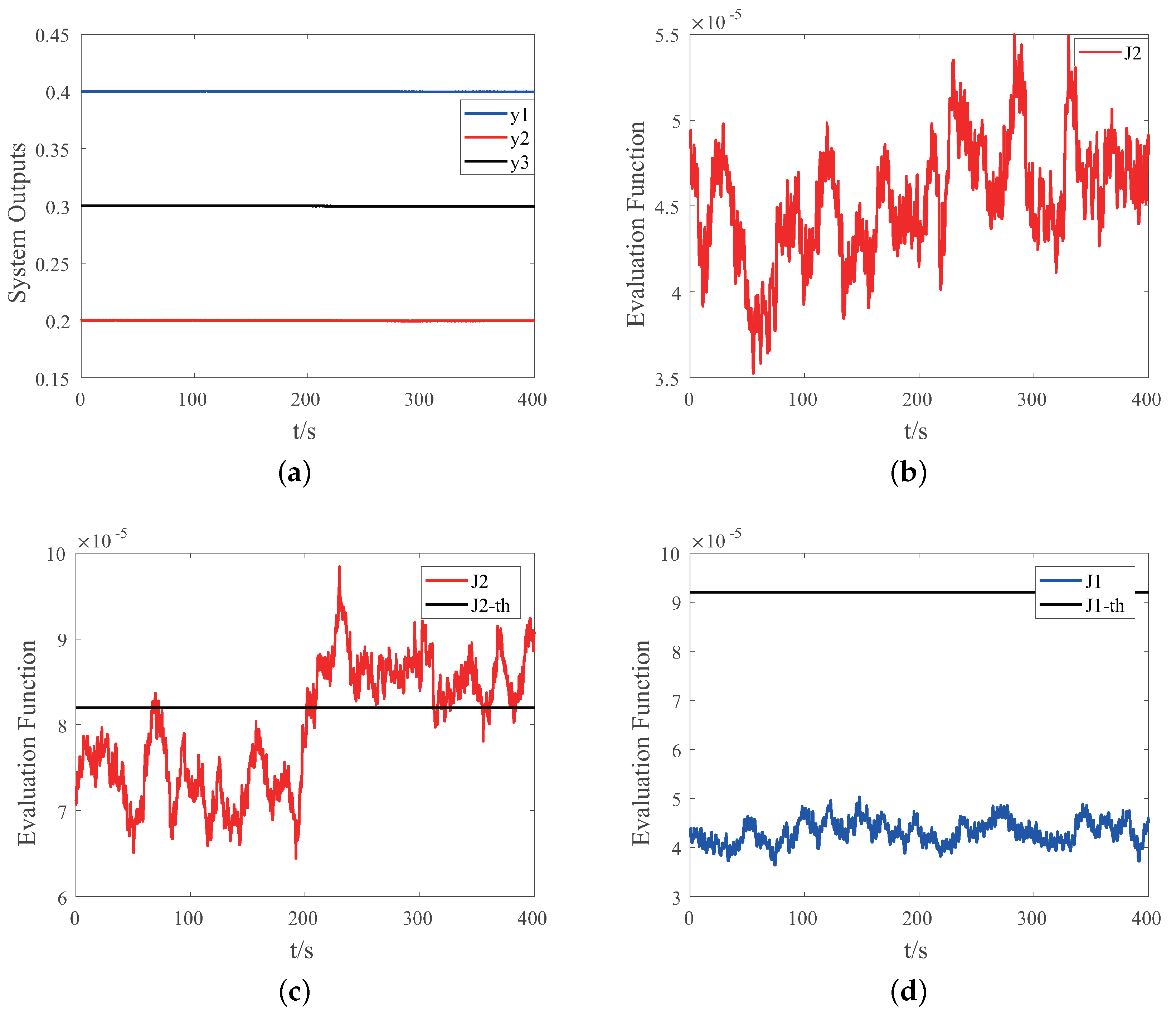
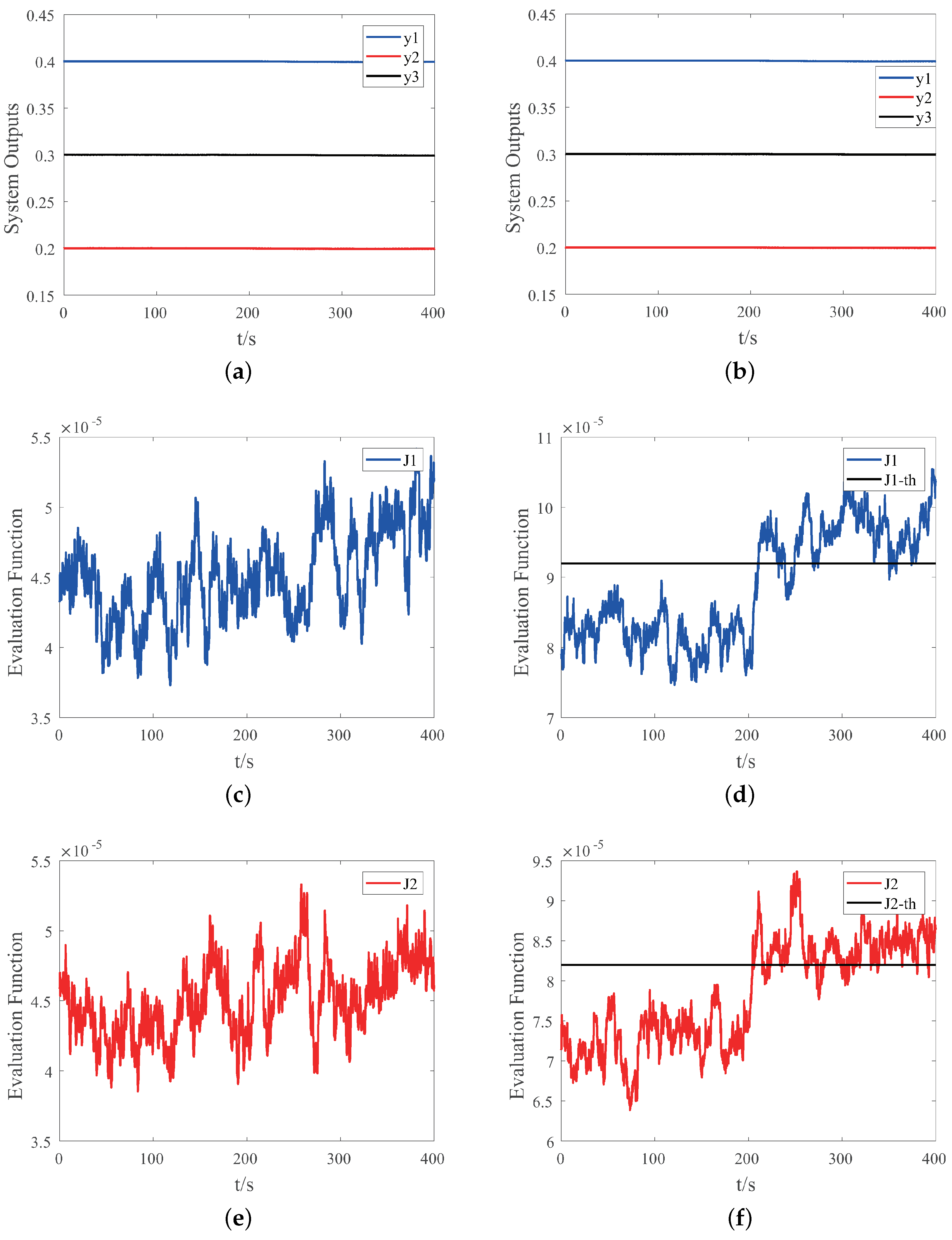
4. Numerical Simulation

In this section, the proposed scheme is applied to the widely used three-tank benchmark system to demonstrate the effectiveness of the strategy [9,33]. As shown in Figure 2, the three-tank system has three outputs $y={[h_1,h_2,h_3]}^T$ and two inputs $u={[u_1,u_2]}^T$.

The target liquid level of three-tank system is $h^{☆}={[0.4,0.2,0.3]}^T$ and two PI controllers are used to control liquid levels $h_1$ and $h_2$ and the parameters are $K_P=1\times {10}^{-5}$ and $K_I=2\times {10}^{-6}$. The nonlinear continuous-time model of the system can be obtained according to the generalized Torricelli Law. Furthermore, the sampling period is set to $T_s=0.1$ s. After linearization and discretization at the equilibrium point, the linear discrete-time system model can be obtained. A detailed process can refer to Appendix A. The system parameters are as follows:

$$\begin{array}{cc}\hfill A^{\left[0\right]}& =\left[\begin{array}{ccc}0.9988649& 0.0000006& 0.0011344\\ 0.0000006& 0.9979022& 0.0011339\\ 0.0011344& 0.0011339& 0.9977311\end{array}\right],\hfill \\ \hfill B^{\left[0\right]}& =\left[\begin{array}{cc}6.4898198& 0.0000014\\ 0.0000014& 6.4866925\\ 0.0036853& 0.0036841\end{array}\right],\hfill \\ \hfill C^{\left[0\right]}& =\left[\begin{array}{ccc}1& 0& 0\\ 0& 1& 0\\ 0& 0& 1\end{array}\right],D_d^{\left[0\right]}=100\times \left[\begin{array}{ccc}1& 0& 0\\ 0& 1& 0\\ 0& 0& 1\end{array}\right],\hfill \\ \hfill B_d^{\left[0\right]}& =\left[\begin{array}{ccc}6.4898198& 0.0000014& 0.0036853\\ 0.0000014& 6.4866925& 0.0036841\\ 0.0036853& 0.0036841& 6.4861359\end{array}\right],\hfill \end{array}$$

$$\begin{array}{cc}\hfill B^{\left[1\right]}& =\left[\begin{array}{cc}6.4898198& 0.0000014\\ 0.0000014& 6.4866925\\ 0.0036853& 0.0036841\end{array}\right]\times \left[\begin{array}{cc}0.99& 0\\ 0& 1\end{array}\right],\hfill \\ \hfill A^{\left[2\right]}& =\left[\begin{array}{ccc}0.9988649& 0.0000006& 0.0011344\\ 0.0000006& 0.9978972& 0.0011339\\ 0.0011344& 0.0011339& 0.9977311\end{array}\right]\hfill \end{array}$$

After transforming the fault models, we get $L^{\left[1\right]}{m}_k^{\left[1\right]}=-0.01\times {[6.4898198,0.0000014,0.0036853]}^T{u}_{1,k}$ and $L^{\left[2\right]}{m}_k^{\left[2\right]}=-{[0,0.000005,0]}^T{x}_{2,k}$, where $u_{1,k}$ is the input of actuator $u_1$ at time k and $x_{2,k}$ is the value of state $x_2$ at time k. Two fault modes can represent actuator fault and system parameter fault, respectively, and the fault signatures $L^{\left[1\right]}$ and $L^{\left[2\right]}$ satisfy Lemma 1. In the simulation experiment, the disturbance is set to be $d_k={[2\times {\varpi }_1,2\times {\varpi }_2,1\times {\varpi }_3]}^T\times sin(k/10)\times {10}^{-6}$, where ${\varpi }_i,i=1,2,3$ are independent random variables uniformly distributed on $[-0.5,0.5]$.

4.1. Simulation Results of the Proposed Method

According to the steps in Section 3.1, the corresponding geometric diagnosis observers are designed as follows:

$$\begin{array}{cc}\hfill F^{\left[1\right]}& =0.9339441,M^{\left[1\right]}=1,G^{\left[1\right]}=\left[\begin{array}{cc}6.4898167& 0\end{array}\right],\hfill \\ \hfill E^{\left[1\right]}& =\left[\begin{array}{ccc}-0.0649202& 0& -0.0010982\end{array}\right],\hfill \\ \hfill H^{\left[1\right]}& =\left[\begin{array}{ccc}0.9999998& 0.0000001& -0.0005682\end{array}\right],\hfill \end{array}$$

$$\begin{array}{cc}\hfill F^{\left[2\right]}& =0.9330108,M^{\left[2\right]}=1,G^{\left[2\right]}=\left[\begin{array}{cc}0& -6.4866894\end{array}\right],\hfill \\ \hfill E^{\left[2\right]}& =\left[\begin{array}{ccc}0& 0.0648908& 0.0010971\end{array}\right],\hfill \\ \hfill H^{\left[2\right]}& =\left[\begin{array}{ccc}-0.0000001& -0.9999998& 0.0005680\end{array}\right]\hfill \end{array}$$

It can be seen that both failure modes are time-invariant, so the auxiliary signals can just select the constant signals to meet the requirements. According to Section 3.2, the auxiliary signals for two faults are designed as $a^{\left[1\right]}={[-7\times {10}^{-7},0]}^T$ and $a^{\left[2\right]}={[0,-6\times {10}^{-7}]}^T$, respectively. The length of the evaluation window is set to be $T_r=10$ s, and the thresholds are selected as $J_{th}^{\left[1\right]}=9.2\times {10}^{-5}$ and $J_{th}^{\left[2\right]}=8.2\times {10}^{-5}$.

Remark 9.

$\parallel B_a^{\left[2\right]}{a}_k^{\left[2\right]}-\alpha L^{\left[2\right]}{m}_k^{\left[2\right]}\parallel \ne 0$ for all α, but it can be very small when selecting proper $a_k^{\left[2\right]}$ and α. Therefore, the diagnosis effect of fault mode $i=2$ is good as well.

Next, the diagnosis results of the proposed method for two fault modes $i=1$ and $i=2$ are introduced.

Case I: When the system is fault-free and both auxiliary signals are put into the system, the simulation results are shown in Figure 3. It can be seen from Figure 3a that the injection of auxiliary signals has very little effect on the system performance because the auxiliary signal itself is much smaller than the input of the system. Figure 3b,c show the evaluation functions before and after the injection of auxiliary signals when the system is fault-free. In practice, the thresholds can be selected as the maximum value of the evaluation functions without faults through multiple tests.

Case II: Assume fault mode $i=1$ occurs at 200 s, and the diagnosis results are shown in Figure 4. Figure 4a shows the system outputs before and after the fault occurrence. It can be seen that the fault is very small and has a slight impact on the system performance. Figure 4b,c respectively show the fault diagnosis results without and with auxiliary signal $a^{\left[1\right]}$, indicating that the auxiliary signal can enhance the performance of fault in residual and greatly enhance the detection ability of incipient fault. Figure 4d is the evaluation function corresponding to observer output $r^{\left[2\right]}$ with auxiliary input $a^{\left[1\right]}$. It can be seen that it is not affected by fault mode $i=1$ and auxiliary signal $a^{\left[1\right]}$, which shows that this method can isolate faults effectively.

Case III: Assume fault mode $i=2$ occurs at 200 s, and the diagnosis results are shown in Figure 5. Similar to Case I, Figure 5a–d show the system outputs, diagnosis results without and with auxiliary signal $a^{\left[2\right]}$ and evaluation function $J^{\left[1\right]}$. Obviously, the proposed method can effectively detect and isolate fault 2 and improve the diagnosis performance.

Case IV: Assume fault modes $i=1$ and $i=2$ occur simultaneously at 200 s, and the diagnosis results are shown in Figure 6. Experimental results indicate that the proposed method can still work well when we aim to actively diagnose both faults simultaneously. Our approach can improve the fault detection performance and realize fault isolation at the same time.

Remark 10.

When two faults occur at the same time, we can input two auxiliary signals in sequence to diagnose the two faults in turn. In addition, the two auxiliary signals in this simulation will not affect each other, so two auxiliary signals can be injected into the system at the same time, and two faults can be detected and isolated at the same time.

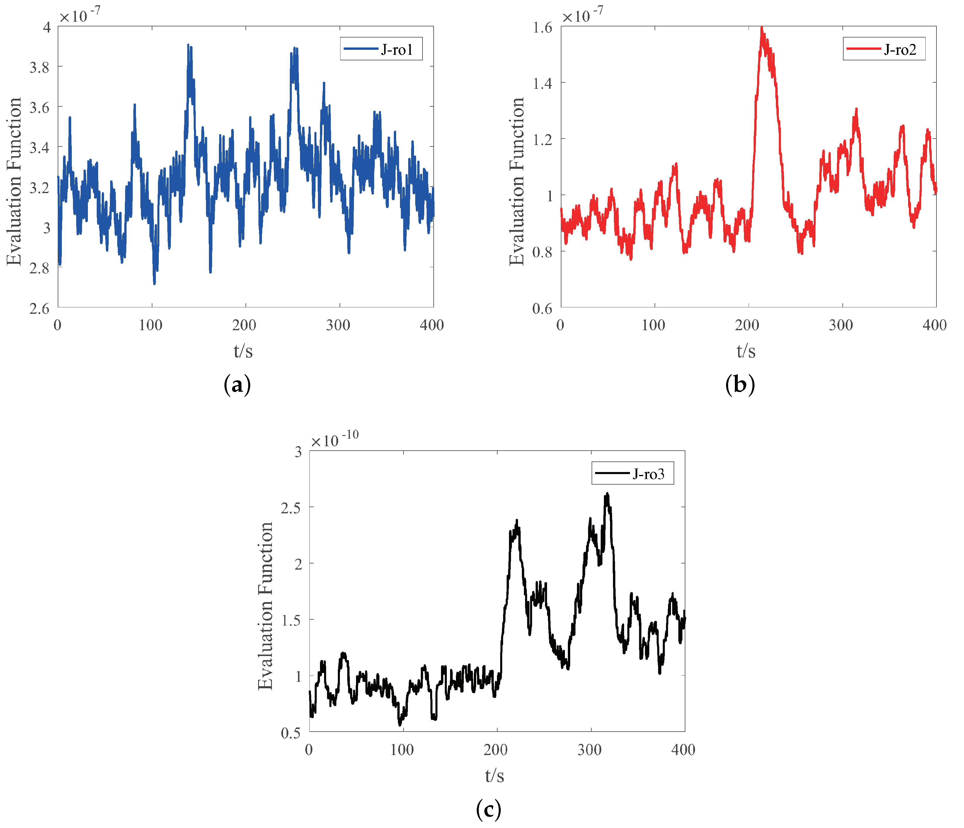
4.2. Compared with Robust Observer

The well-known robust observer in [34] is also a method that can detect and isolate faults simultaneously. Robust observer is a kind of passive fault diagnosis method, and it is used as a comparison method in this section. According to the method proposed in reference [34], if we want to detect and isolate three kinds of component faults when we use two measures $y_1$ and $y_2$, three robust observers need to be designed. The detailed design process of robust observer is omitted here. For convenience, two kinds of fault types are considered in this section, and the corresponding simulation results are listed for comparison. The same evaluation function in Section 3.3 is used to process the residual.

Case I: Consider the same failure mode $i=1$ as in Section 4.1. The diagnosis results of robust observer are shown in Figure 7. If the output of the second observer and the third observer exceed the selected thresholds at the same time, then it is judged that the fault has occurred. It can be seen from Figure 7b,c that the outputs of the two observers fluctuate greatly after fault $i=1$ occurs, which makes it impossible to diagnose the fault effectively. Compared with Figure 4c, it can be seen that the method in this paper has better diagnostic performance for fault mode $i=1$.

Case II: In this case, assume that actuator 2 fails as the third failure mode $i=3$.

$$\begin{array}{c}\hfill B^{\left[3\right]}=\left[\begin{array}{cc}6.4898198& 0.0000014\\ 0.0000014& 6.4866925\\ 0.0036853& 0.0036841\end{array}\right]\times \left[\begin{array}{cc}1& 0\\ 0& 0.99\end{array}\right]\end{array}$$

After transforming the fault models, we get $L^{\left[3\right]}{m}_k^{\left[3\right]}=-0.01\times {[0.0000014,6.4866925,0.0036841]}^T{u}_{2,k}$, where $u_{2,k}$ is the input of actuator $u_2$ at time k. The simulation results are shown in Figure 8 and Figure 9. In the robust observer method, it is judged that the fault has occurred if the output of the first observer and the third observer exceed the selected thresholds at the same time. It can be seen that the proposed method has better performance in fault diagnosis of fault mode $i=3$ compared with the robust observer.

5. Conclusions

This paper has investigated the fault-structure-based AFD problem for the LTI systems using a geometric observer. The observer designed based on geometric method is only sensitive to faults in specific direction, so it can be used to monitor the fault with specific structure. According to the residual formula of the observer, the auxiliary signals have been designed to enhance the fault diagnosis performance. In addition, the requirements that the auxiliary signals need to meet have been discussed. In this paper, the geometric approach based fault diagnosis observer has been applied to active fault diagnosis for the first time, which can realize the seamless combination of active fault diagnosis and passive fault diagnosis. Simulation experiments have been carried out based on the three-tank system. The simulation results have shown that the proposed method significantly improved the diagnosis performance of incipient faults. In the future, we aim to consider the problem of fault estimation when the fault amplitude is unknown.

References

1. He, X.; Guo, Y.Q.; Zhang, Z.; Jia, F.L.; Zhou, D.H. Active fault diagnosis for dynamic systems. Acta Autom. Sin. 2020, 46, 1557–1570. [Google Scholar]
2. Zhang, K.; Zhou, D.H.; Chai, Y. Review of multiple fault diagnosis methods. Acta Autom. Sin. 2015, 32, 1143–1157. [Google Scholar]
3. Gao, Z.W.; Cecati, C.; Ding, S.X. A survey of fault diagnosis and fault-tolerant techniques—Part I: Fault diagnosis with model-based and signal-based approaches. IEEE Trans. Ind. Electron. 2015, 62, 3757–3767. [Google Scholar] [CrossRef] [Green Version]
4. Liu, Q.; Zhou, J.; Lang, Z.Q.; Qin, S.J. Perspectives on data-driven operation monitoring and selfoptimization of industrial processes. Acta Autom. Sin. 2018, 44, 1944–1956. [Google Scholar]
5. Wang, H.; Wang, H.B.; Jiang, G.Q.; Li, J.M.; Wang, Y.L. Early fault detection of wind turbines based on operational condition clustering and optimized deep belief network modeling. Energies 2019, 12, 984. [Google Scholar] [CrossRef] [Green Version]
6. Mao, Z.H.; Yan, X.G.; Jiang, B.; Chen, M. Adaptive fault-tolerant sliding-mode control for high-speed trains with actuator faults and uncertainties. IEEE Trans. Intell. Transp. Syst. 2020, 21, 2449–2460. [Google Scholar] [CrossRef] [Green Version]
7. Xue, T.; Zhong, M.Y.; Li, L.L.; Ding, S.X. An optimal data-driven approach to distribution independent fault detection. IEEE Trans. Ind. Inform. 2020, 16, 6826–6836. [Google Scholar] [CrossRef]
8. Piltan, F.; Kim, C.H.; Kim, J.M. Advanced adaptive fault diagnosis and tolerant control for robot manipulators. Energies 2019, 12, 1281. [Google Scholar] [CrossRef] [Green Version]
9. He, X.; Wang, Z.D.; Liu, Y.; Qin, L.G.; Zhou, D.H. Fault tolerant control for an Internet-based Three-tank system: Accommodation to sensor bias faults. IEEE Trans. Ind. Electron. 2017, 64, 2266–2275. [Google Scholar] [CrossRef]
10. Heirung, T.A.N.; Mesbah, A. Input design for active fault diagnosis. Annu. Rev. Control 2019, 47, 35–50. [Google Scholar] [CrossRef]
11. Zhang, X.J.; Zarrop, M.B. Auxiliary signals for improving online fault detection. In Proceedings of the International Conference on Control, Oxford, UK, 13–15 April 1988. [Google Scholar]
12. Puncochar, I.; Skach, J. A survey of active fault diagnosis methods. IFAC-PapersOnLine 2018, 51, 1091–1098. [Google Scholar] [CrossRef]
13. Wang, J.; Zhang, J.J.; Qu, B.; Wu, H.Y.; Zhou, J.L. Unified architecture of active fault detection and partial active fault-tolerant control for incipient faults. IEEE Trans. Syst. Man. Cybern.-Syst. 2017, 47, 1688–1700. [Google Scholar] [CrossRef]
14. Marseglia, G.R.; Raimondo, D.M. Active fault diagnosis: A multi-parametric approach. Automatica 2017, 79, 223–230. [Google Scholar] [CrossRef]
15. Lin, F.; Wang, L.Y.; Chen, W.; Han, L.; Shen, B. N-diagnosability for active online diagnosis in discrete event systems. Automatica 2017, 83, 220–225. [Google Scholar] [CrossRef]
16. Nikoukhah, R.; Campbell, S.L. Auxiliary signal design for active failure detection in uncertain linear systems with a priori information. Automatica 2006, 42, 219–228. [Google Scholar] [CrossRef]
17. Wang, Y.; Olaru, S.; Valmorbida, G.; Puig, V.; Cembrano, G. Set-invariance characterizations of discrete-time descriptor systems with application to active mode detection. Automatica 2019, 107, 255–263. [Google Scholar] [CrossRef]
18. Heirung, T.A.N.; Mesbah, A. Stochastic nonlinear model predictive control with active model discrimination: A closed-loop fault diagnosis application. IFAC-PapersOnLine 2017, 50, 15934–15939. [Google Scholar] [CrossRef]
19. Blackmore, L.; Rajamanoharan, S.; Williams, B. Active estimation for jump markov linear systems. IEEE Trans. Autom. Control 2008, 53, 2223–2236. [Google Scholar] [CrossRef] [Green Version]
20. Yang, J.W.; Hamelin, F.; Sauter, D. Active fault diagnosis based on a framework of optimization for closed loop system. In Proceedings of the 2014 International Conference on Control, Decision and Information Technologies, Metz, France, 3–5 November 2014; pp. 387–392. [Google Scholar]
21. Blanchini, F.; Casagrande, D.; Giordano, G.; Miani, S.; Olaru, S.; Reppa, V. Active fault isolation: A duality-based approach via convex programming. SIAM J. Control Optim. 2017, 55, 1619–1640. [Google Scholar] [CrossRef] [Green Version]
22. Scott, J.K.; Findeisen, R.; Braatz, R.D.; Raimondo, D.M. Input design for guaranteed fault diagnosis using zonotopes. Automatica 2014, 50, 1580–1589. [Google Scholar] [CrossRef]
23. Scott, J.K.; Raimondo, D.M.; Marseglia, G.R.; Braatz, R.D. Constrained zonotopes: A new tool for set-based estimation and fault detection. Automatica 2016, 69, 126–136. [Google Scholar] [CrossRef]
24. Raimondo, D.M.; Marseglia, G.R.; Braatz, R.D.; Scott, J.K. Closed-loop input design for guaranteed fault diagnosis using set-valued observers. Automatica 2016, 74, 107–117. [Google Scholar] [CrossRef]
25. Karami, H.; Ghasemi, R.; Mohammadi, F. Adaptive neural observer-based nonsingular terminal sliding mode controller design for a class of nonlinear sytems. In Proceedings of the International Conference on Control, Instrumentation, and Automation, Sanandaj, Iran, 30–31 October 2019. [Google Scholar]
26. Manouchehri, P.; Ghasemi, R.; Toloei, A.; Mohammadi, F. Distributed neural observer-based formation strategy of affine nonlinear multi-agent systems with unknown dynamics. J. Circuits Syst. Comput. 2020. [Google Scholar] [CrossRef]
27. Massoumnia, M.A.; Verghese, G.C.; Willsky, A.S. Failure detection and identification. IEEE Trans. Autom. Control 1989, 34, 316–321. [Google Scholar] [CrossRef]
28. Meskin, N.; Khorasani, K. A geometric approach to fault detection and isolation of continuous-time Markovian jump linear systems. IEEE Trans. Autom. Control 2010, 55, 1343–1357. [Google Scholar] [CrossRef] [Green Version]
29. Longhi, S.; Monteriu, A. Fault detection and isolation of linear discrete-time periodic systems using the geometric approach. IEEE Trans. Autom. Control 2017, 62, 1518–1523. [Google Scholar] [CrossRef]
30. Hammouri, H.; Kabore, P.; Kinnaert, M. A geometric approach to fault detection and isolation for bilinear systems. IEEE Trans. Autom. Control 2001, 46, 1451–1455. [Google Scholar] [CrossRef]
31. Bokor, J.; Balas, G. Detection filter design for LPV systemsła geometric approach. Automatica 2004, 40, 511–518. [Google Scholar] [CrossRef]
32. Yu, L. Robust Control: Linear Matrix Inequality Method; Tsinghua University Press: Beijing, China, 2002. [Google Scholar]
33. Zhou, D.H.; He, X.; Wang, Z.D.; Liu, G.P.; Ji, Y.D. Leakage fault diagnosis for an internet-based three-tank system: An experimental study. IEEE Trans. Control Syst. Technol. 2012, 20, 857–870. [Google Scholar] [CrossRef]
34. Ge, W.; Fang, C.Z. Detection of faulty components via robust observation. Int. J. Control 1988, 47, 581–599. [Google Scholar] [CrossRef]
Figure 1. Framework of the fault-structure-based active fault diagnosis.
Energies 13 04475 g001
Figure 2. Structure of the three-tank system [33].
Energies 13 04475 g002
Figure 3. Simulation results of the system without faults and two auxiliary signals a [ 1 ] and a [ 2 ] are injected into the system at 200 s: (a) system outputs; (b) the evaluation function of the residual r [ 1 ] and the corresponding threshold; (c) the evaluation function of the residual r [ 2 ] and the corresponding threshold.
Energies 13 04475 g003
Figure 4. Simulation results of the system with fault mode i = 1 occurring at 200 s: (a) system outputs without auxiliary signals; (b) the evaluation function J [ 1 ] without auxiliary signals; (c) the evaluation function J [ 1 ] with auxiliary signal a [ 1 ] ; (d) the evaluation function J [ 2 ] with auxiliary signal a [ 1 ] .
Energies 13 04475 g004
Figure 5. Simulation results of the system with fault mode i = 2 occurring at 200 s: (a) system outputs without auxiliary signals; (b) the evaluation function J [ 2 ] without auxiliary signals; (c) the evaluation function J [ 2 ] with auxiliary signal a [ 2 ] ; (d) the evaluation function J [ 1 ] with auxiliary signal a [ 2 ] .
Energies 13 04475 g005
Figure 6. Simulation results of the system with fault modes i = 1 and i = 2 occurring simultaneously at 200 s: (a) system outputs without auxiliary signals; (b) system outputs with auxiliary signals; (c) the evaluation function J [ 1 ] without auxiliary signals; (d) the evaluation function J [ 1 ] with auxiliary signals; (e) the evaluation function J [ 2 ] without auxiliary signals; (f) the evaluation function J [ 2 ] with auxiliary signals.
Energies 13 04475 g006
Figure 7. Simulation results of robust observer with fault modes i = 1 occurring at 200 s: (a) evaluation function of the first robust observer; (b) evaluation function of the second robust observer; (c) evaluation function of the third robust observer.
Energies 13 04475 g007
Figure 8. Simulation results of robust observer with fault modes i = 3 occurring at 200 s: (a) evaluation function of the first robust observer; (b) evaluation function of the second robust observer; (c) evaluation function of the third robust observer.
Energies 13 04475 g008
Figure 9. Simulation results of the proposed method with fault modes i = 3 occurring at 200 s: (a) the evaluation function J [ 1 ] with auxiliary signals. (b) the evaluation function J [ 2 ] with auxiliary signals.
Energies 13 04475 g009