Structural Vector Autoregressive Approach to Evaluate the Impact of Electricity Generation Mix on Economic Growth and CO₂ Emissions in Iran

Abstract

This research attempts to evaluate the impact of renewable electricity generation mix on economic growth and CO₂ emissions in Iran from 1980 to 2016. In this regard, by using EViews 10, the Structural Vector Autoregressive model (SVAR) is estimated by imposing the Blanchard and Quah long-run restrictions. The yearly data on real Gross Domestic Production (GDP), the share of electricity generation from renewable sources, and carbon dioxide emissions (CO₂) caused by liquid, solid, and gaseous fuels were used. The positive impact of one standard deviation shock of increasing the share of renewable electricity on economic growth was confirmed by using Impulse Response Function (IRF). Contrary to the expectation, the share of renewable electricity in the energy mix is not at a desirable level to lower CO₂ emissions, which partly could be explained by the dominant role of fossil fuel in Iran (as an energy-driven country). Moreover, the findings of Variance Decomposition (VD) verified the low share of electricity generated by renewable energy in explaining forecast error variations in economic growth and CO₂ emissions. It indicates that in this stage of development, increasing the share of renewable electricity could not be considered as an appropriate strategy to control environmental issues. Therefore, initiating and implementing environmental policies could be considered as the most proper policies to lower CO₂ emissions and to achieve the goal of sustainable development.

1. Introduction

Recently, greenhouse gas emissions, caused by the overconsumption of fossil fuels, have become the most concerning environmental problem around the world, especially in developing countries [1]. Indeed, global energy consumption and environmental concerns might be affected by patterns of energy consumption and production of these countries, which originate from their rapid economic development and large population [2]. It is worthwhile to mention that despite the vital role of energy in economic growth, the environmental side effects of increasing energy consumption, especially in the early stage, need to be considered to achieve the goals of sustainable development.

Review of the relationship between economic growth and energy consumption has drawn researchers’ attention, particularly after the oil crisis in the 1970s. Although the development stage, sample size, country, studied variables, and econometric methods have led to varied results, all studies have confirmed the linkage between Gross Domestic Production (GDP), as a proxy of economic growth, and energy consumption [3]. While some studies have postulated the unidirectional causality running from economic growth to energy consumption (the growth hypothesis) or vice versa (the conservation hypothesis), others have identified no interaction (the neutrality hypothesis) or bidirectional causality (the feedback hypothesis) [4]. Furthermore, the relationship between economic growth and environmental quality has been widely investigated since the 1990s. Initially, this relationship was derived from the seminal work of Kuznets [5]. He showed that income inequality increases along with income growth, stabilizes, and then decreases, indicating the inverted-U shaped relationship between variables studied. Inspired by this concept, environmental economists have postulated the relationship between income growth and environmental degradation. After that, the first attempt dates back to the seminal works of Grossman and Krueger [6], Shafik and Bandyopadhyay [7], Panayotou [8], and Selden and Song [9]. They confirmed the inverted-U shaped relationship between economic growth and environmental deterioration and called it the Environmental Kuznets Curve (EKC).

As stated before, in the early stage of economic growth, the positive impact of energy consumption on economic growth is accompanied by upward trends in greenhouse gas emissions. This dilemma led to the emerging concept of sustainable development. Achieving this level of development needs to minimize the side effects, which decrease natural resources and environmental quality [10]. Investigating energy consumption has drawn more attention after countries’ consensus on energy conservation and greenhouse gas reduction based on sustainable development. Therefore, shifting away from fossil fuels to renewable energies has gained more attention to achieve these goals. To our best knowledge, so far, there is no conclusive result in the current literature on the exact role of renewable energy in economic growth and environmental degradation. The most related studies are illustrated in

Table 1. Summary of empirical studies.

Reference	Country (ies)	Methodology (ies)	Impact of Renewable Energy/Electricity on
			Economic Growth	CO2 Emissions
[11]	India	SVAR	+	−
[12]	The US, Denmark, Portugal, Spain	SVAR	− except for the US	−
[13]	China, India, Japan	SVAR	China (SR): − LR: +
[14]	Vietnam	ARDL		No effect
[15]	Latin American and the Caribbean countries	FMOLS, VECM Granger Causality	Feedback hypothesis	No effect
[16]	Iran	ARDL, VECM, DOLS, FMOLS	+
[17]	42 developing (Iran)	Panel Data	+
[18]	Turkey	ARDL, FMOLS, CCR		No effect
[19]	8 South American	ARDL		−
[20]	16 EU-countries	PMG-ARDL		−

+ and − indicate the positive and negative impacts of renewable energy/electricity on investigated variables.

.

To the best of the authors’ knowledge, no research has been conducted to investigate the impact of unit standard deviation innovation of renewable electricity on economic growth and CO₂ emissions in the fossil fuel-based country with huge potential in renewable energies, high levels of CO₂ emissions, and commitment to lower the environmental issues, such as Iran. Therefore, this research aims to fill this gap by considering three variables (real GDP, the share of renewable energy in energy mix, and CO₂ emissions) from 1980 to 2016 using the SVAR method.

Being located between two major world energy focus areas, the Persian Gulf and the Caspian Sea, has given Iran a strategic position in energy supply and security. Indeed, ranking as the second and the fourth gas (accounts for 9.3 percent of world gas reserves) and oil holder (having 17.2 percent of the total world’s affordable oil condensate reserves) in 2017, Iran is considered an energy-driven economy [21]. Moreover, it has numerous potentials in renewable energies due to its location in one of the World’s Sun Belts, enjoying 2800 sunny hours per year and an average 2000 kWh/m² solar insulation [22], and on the world’s Geothermal Belt. However, the share of renewable energy in the total energy mix (2 percent) and electricity generation has remained low [21], which has increased the concerns about environmental degradation. To solve this issue, the government must consider critical measures to decrease the high dependency on fossil fuels and to diversify the energy mix. This study intends to answer the following questions:

• How does electricity generated by renewable sources contribute to the economic growth of Iran?
• How is carbon dioxide affected by unit standard deviation shock of renewable electricity?
• What is the contribution of renewable electricity in explaining forecast error variance decomposition of economic growth and carbon dioxide emissions?
• What is an appropriate energy policy for Iran as an energy driven country?

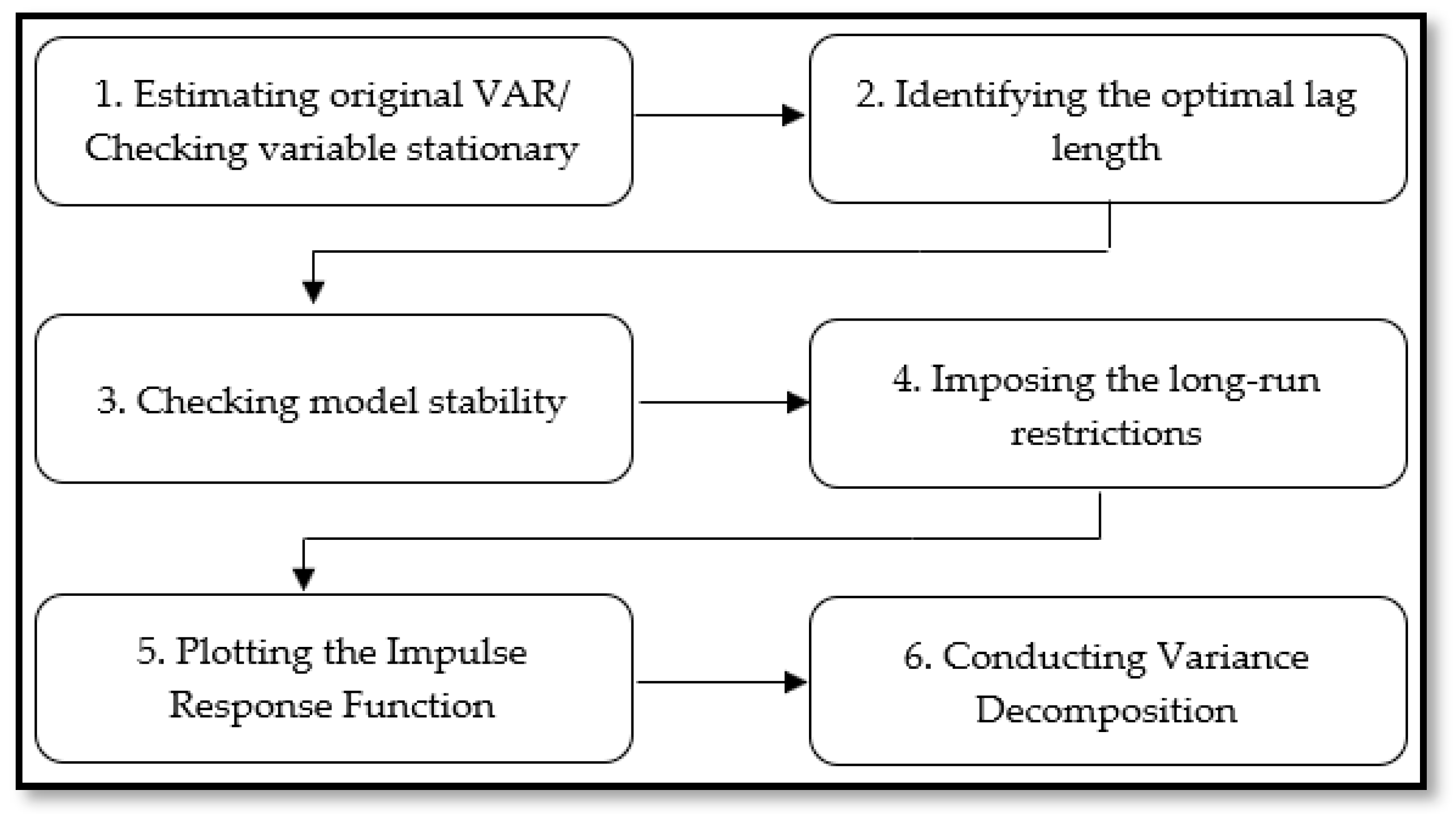
The rest of the paper is organized as follows. Section 2 reports the data and methodology. Section 3 discusses the conceptual framework including the empirical findings. Finally, the paper ends up with pointing out the conclusion and policy implication in Section 4.

2. Methodology

Sims (1980) proposed an alternative to the large scale macro-econometric time series model, called Vector Autoregressive (VAR). This model does not rely on incredible identifying assumptions [23]. In the initial version, the impulse response functions were obtained from Cholesky decomposition. Since this decomposition method implied a causal ordering, achieving the incredible results were unacceptable, when more than monetary shocks were considered [24]. To overcome this obstacle, Bernanke [25], Blanchard Watson [26], and Sims [27] developed the SVAR model by imposing theoretical constraints on the simultaneous impacts of impulses. Later on, Clarida and Gali [28] recognized the impulse response functions by imposing the theoretical constraints on the long-run impacts of impulses. Shortly, to identify the system and achieve economic interpretable impulse response functions and to evaluate the impact of pursuing specific policy measures or significant changes in the economy, the SVAR model was applied by imposing restrictions based on economic theory [13]. The conceptual framework is illustrated in Figure 1.

From Figure 1, examining the impact of electricity generation mix on GDP and environmental quality needed to take six steps as follows:

• Checking variables stationary through conducting KPSS unit root tests [29] and estimating the original VAR model.
• Identifying the optimal lag length using several criteria.
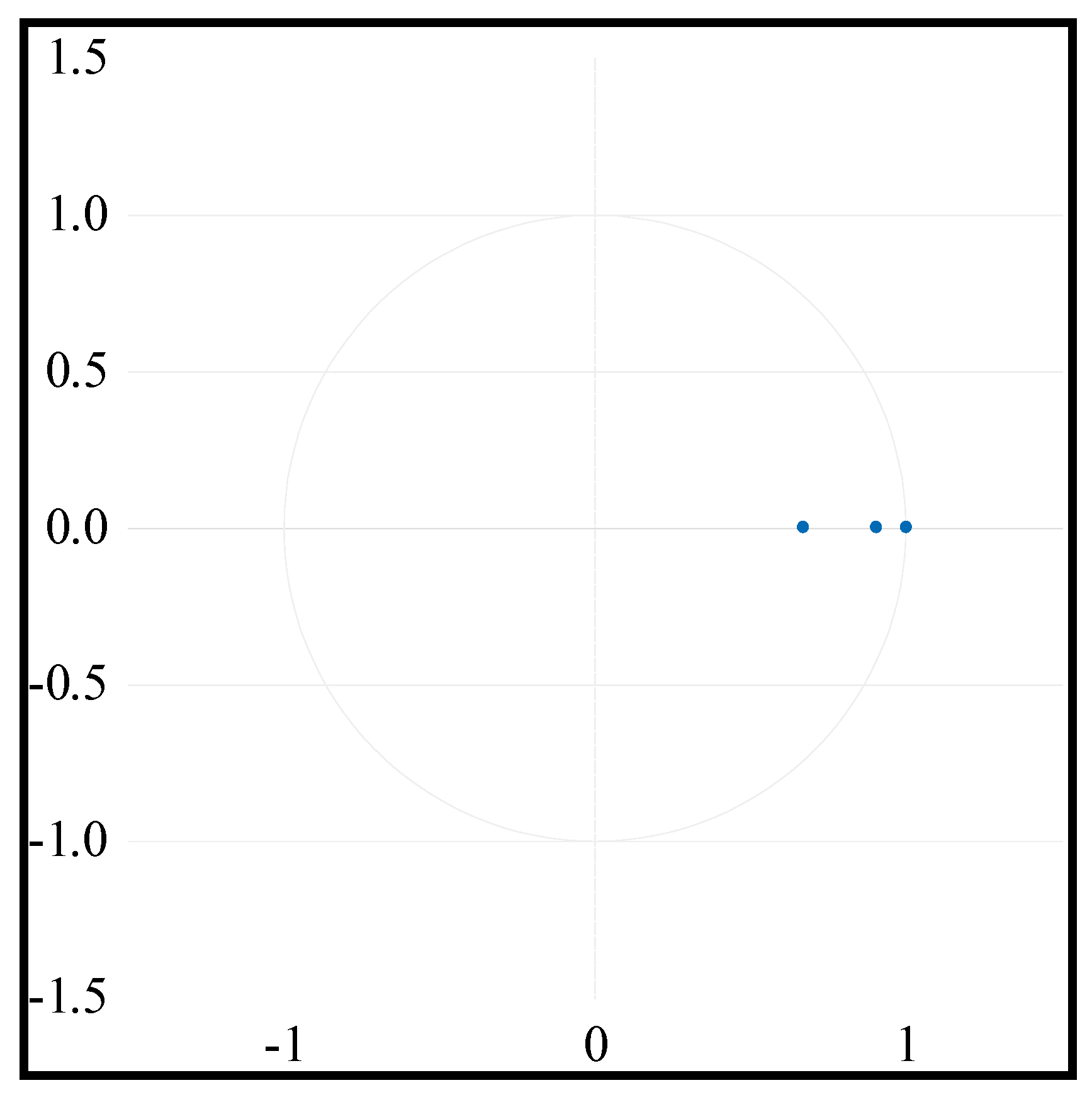
• Checking model stability by employing inverse roots of the characteristic polynomials.
• Imposing the Blanchard and Quah long-run restrictions [30] based on the literature review and economic theory.
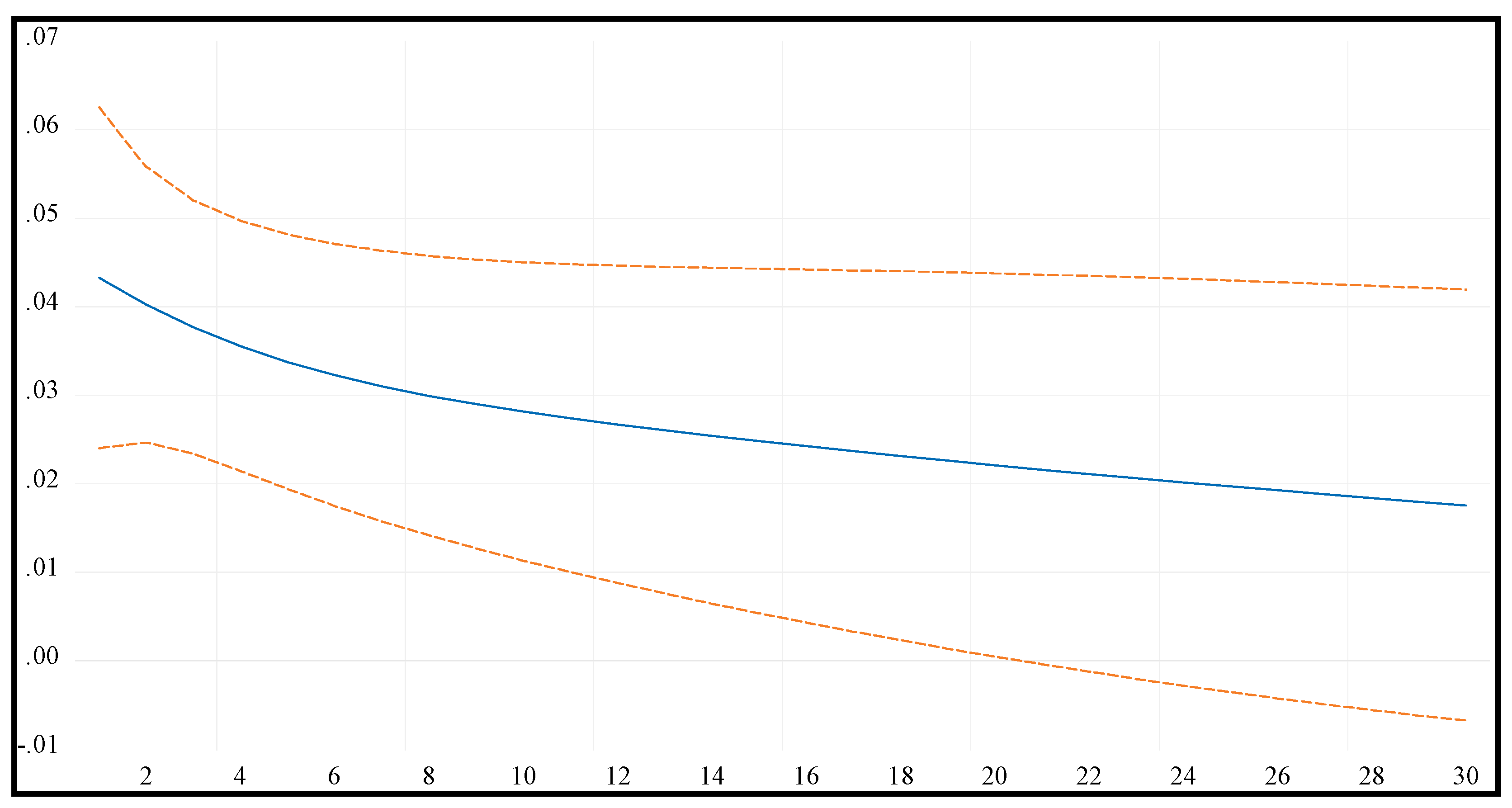
• Plotting the IRFs to consider the dynamic responses of endogenous variables to a unit standard deviation shock of some of the other variables in the system over time.
• Conducting VD to identify the importance of each exogenous shock in explaining the forecast error variance of each variable.

2.1. Structural Vector Autoregressive Model

The analysis starts by investigating the relationship between prediction errors ($u_t$), and structural disturbance (${\epsilon }_t$) in the VAR model of order $p$ (VAR ($p$)) with $K$ endogenous variables using Equation (1) [25,27].

$$y_t=\nu +A_1{y}_{t-1}+\cdots +A_p{y}_{t-p}+u_t=A{\acute{Y}}_{t-1}+u_t$$

(1)

where$\nu$ is $K\times 1$ vector and stands for fixed, no stochastic drift component. ${\acute{Y}}_{t-1}\equiv \left(1,{\acute{y}}_{t-1},\cdots ,{\acute{y}}_{t-p}\right)$is $\left(Kp+1\right)$dimensional. $A\equiv \left(\nu ,A_1,\cdots ,A_p\right)$ is $K\times \left(Kp+1\right)$; $u_t=\acute{\left(u_{1t},\cdots ,u_{Kt}\right)}$ is a $K$-dimensional white noise residuals process. Therefore, it is not correlated serially, has zero mean and covariance matrix ${{\displaystyle \sum }}^{}u$.

By multiplying the Equation (1) by an invertible $\left(K\times K\right)$ matrix $A$, the structural relationships between the variables are obtained as follows:

$$A{y}_t=A\nu +A{A}_1{y}_{t-1}+\cdots +A{A}_p{y}_{t-p}+A{u}_t=AA{Y}_{t-1}+A{u}_t$$

$A{u}_t=w_t={(w_{1t},\cdots ,w_{Kt})}^{/}$ indicates the structural innovation (shocks), assuming that $A$ has a unit main diagonal and $w_t~(0,{{\displaystyle \sum }}^{}w)$ has a diagonal covariance matrix ${{\displaystyle \sum }}^{}w=A{{\displaystyle \sum }}^{}u\stackrel{`}{A=}diag\left({\sigma }_1^2,\cdots ,{\sigma }_K^2\right)$. Consequently, specifying the $i{j}^{th}$ element of $A$ by $a_{ij}$, the kth structural equation is as follows:

$$y_{kt}=-{\displaystyle \sum }_{\begin{array}{c}i=1\\ i\ne k\end{array}}^K{a}_{ki}{y}_{it}+a_k^{\ast }{Y}_{t-1}+w_{kt}$$

where $a_k^{\ast }$ shows the kth row of $AA$.

To ensure identifying properties of matrix $A$ and estimating its consistency, the constraints should be imposed on this matrix, which are called the A-model by [31].

Specifying $w_t=B^{-1}{u}_t$ or $u_t=B{w}_t$ and regarding the structural form, the structure can be imposed using Equation (2).

$$y_t=\nu +A_1{y}_{t-1}+\cdots +A_p{y}_{t-p}+B{w}_t=A{\acute{Y}}_{t-1}+B{w}_t$$

(2)

In Equation (2), $u_t$, the reduced-form innovations are substituted by $B{w}_t$, assuming $w_t$ have a unit covariance matrix such that $w_t~\left(0,I_K\right)$, and ${{\displaystyle \sum }}^{}u=B\acute{B}$, which is named B-model. In this model, the identifying restrictions are imposed on the structural matrix $B$, which implies the short run impacts of the structural shocks ($w_t)$.

Considering the combination of the A- and B-model is a way to facilitate imposing the identifying restrictions, Equation (3), which referred to the AB-model by [32] is

$$A{y}_t=A\nu +A{A}_1{y}_{t-1}+\cdots +A{A}_p{y}_{t-p}+B{w}_t=AA{\acute{Y}}_{t-1}+B{w}_t$$

(3)

In Equation (3), $w_t~\left(0,I_K\right)$, and ${{\displaystyle \sum }}^{}u=A^{-1}B\acute{B{A}^{-1}}$ [33].

2.2. Imposing Long-Run Restrictions

The long-run impacts of shocks are the accumulated impacts of the shocks, which are zero in the stable and stationary VAR models. Denoting $A\left(1\right)\equiv I_K-A_1-\cdots -A_p$, the relevant long-run multiplier matrix is written as Equation (4).

$$\mathsf{\Xi }=A{\left(1\right)}^{-1}{A}^{-1}B$$

(4)

The B-model with long-run multiplier matrix $\mathsf{\Xi }=A{\left(1\right)}^{-1}B$ is commonly used in practice [34]. According to Blanchard and Quah [30], triangular matrix is the most general set of constraints, which restrains Ξ. The linear restrictions on Ξ in B-model can be illustrated as follows:

$$Q^{l}vec\left(\mathsf{\Xi }\right)=Q^l\left(A{\left(1\right)}^{-1,}⨂ I_K\right) vec\left(B\right)=q^l$$

where $Q^l$, and $q^l$ stand for a suitable known restriction matrix and a suitable vector, respectively. Consequently, given the reduced-form parameters, the implied restrictions for the structural parameters $B$ are linear restrictions with restriction matrix as Equation (5).

$$\mathrm{Q}=Q^l\left(A{\left(1\right)}^{-1,}⨂ I_K\right)$$

(5)

In a model with integrated and co-integrated variables, a shock has lasting impacts on the variables. In this case, the long-run effects matrix for the B-model is as follows:

$$\mathsf{\Xi }={\beta }_{\perp }{\left[{\stackrel{`}{\alpha }}_{\perp }\left(I_K-{\displaystyle \sum }_{i=1}^{p-1}{\mathsf{\Gamma }}_i\right){\beta }_{\perp }\right]}^{-1}{\stackrel{`}{\alpha }}_{\perp }B$$

${\beta }_{\perp }$, and ${\alpha }_{\perp }$ are orthogonal complements of $\beta$, and $\alpha$, respectively [33]. In the same way, $B$ must be replaced by $A^{-1}$ or by $A^{-1}B$ for the $A$- and $AB$ model, respectively.

2.3. Model Specification

To investigate the impact of the mix of renewable electricity on economic growth and CO₂ emissions, in this research, the long-run constraints method was applied, in which vector Y(t) includes intended variables as Equation (6).

$$y_t=\left(RES LGDP, LC{O}_2\right)$$

(6)

Three structural impulses are imposed on the model Equation (7).

$${\epsilon }_t=\left({\epsilon }^{RES}, {\epsilon }^{LGDP},{\epsilon }^{LC{O}_2} \right)$$

(7)

where ${\epsilon }^{RES}$ stands for the logarithm of renewable electricity generation impulse. ${\epsilon }^{LGDP}$ indicates for the logarithm of real gross domestic production impulse. ${\epsilon }^{LC{O}_2}$ represents the logarithm of carbon dioxide emissions impulse.

The long-run structural innovation in the matrix form can be shown as Equation (8).

$$\left[\begin{array}{c}RES\\ LGDP\\ LC{O}_2\end{array}\right]=\left[\begin{array}{c}{C}_{11}\left(L\right) C_{12}\left(L\right) C_{13}\left(L\right)\\ C_{21}\left(L\right) C_{22}\left(L\right) C_{23}\left(L\right)\\ C_{31}\left(L\right) C_{32}\left(L\right) C_{33}\left(L\right)\end{array}\right]\left[\begin{array}{c}{\epsilon }^{LRES}\\ {\epsilon }^{LGDP}\\ {\epsilon }^{LC{O}_2}\end{array}\right]$$

(8)

In this matrix $C\left(L\right)={\displaystyle \sum }_{J=0}^{\infty }{C}_J\left(L\right)$.

Following [11,12,13], it assumed that there is a one-sided relation from renewable electricity generation to real GDP and CO₂ emissions, and from real GDP to CO₂ emissions (Figure 2).

The long-run restrictions introduced by [30] are imposed on Equation (8). The lower triangular matrix is obtained (Equation (9)).

$$C\left(L\right)=\left[\begin{array}{c}{C}_{11}\left(L\right) 0 0\\ C_{21}\left(L\right) C_{22}\left(L\right) 0\\ C_{31}\left(L\right) C_{32}\left(L\right) C_{33}\left(L\right)\end{array}\right]$$

(9)

3. Data and Empirical Finding

3.1. Data

The yearly data was used over 1980–2016 to investigate the impact of expanding the share of renewable electricity on GDP and CO₂ emissions. GDP is the real gross domestic production (billions constant 2010 US$); RES stands for the share of renewable energy in the electricity generation mix, measured in billion Kwh, following Hdom [19]; and $\mathrm{CO}$₂ is the per capita emissions of carbon dioxide caused by solid, liquid, and gas fuel consumption, measured in metric tons. The data of real GDP was retrieved from the World Development Indicator database [35], and the data of CO₂ emissions and the share of renewable sources in electricity generation were sourced from the U.S. Energy Information Administration [36]. To reduce the data variability and to avoid the heteroscedasticity problem in the error terms, the data were converted to the logarithm form [37], except RES. The descriptive statistics of studied variables are summarized in

Table 2. Descriptive statistic.

	RES	LGDP	LCO2
Mean	9.575796	5.726277	5.689736
Median	7.264000	5.680259	5.680323
Maximum	22.45900	6.214520	6.467844
Minimum	3.662000	5.168314	4.695737
Std. Dev.	4.910548	0.327201	0.530751
Skewness	1.124100	0.038299	−0.090554
Kurtosis	3.008702	1.706429	1.851405
Jarque–Bera	7.581718	2.518792	2.028106
Probability	0.022576	0.283825	0.362746
Sum	344.7286	206.1460	204.8305
Sum Sq. Dev.	843.9720	3.747111	9.859376

L shows the logarithm form of the studied variables.

.

From Table 2, renewable electricity had the highest mean value and standard deviation. Accordingly, the lowest mean value and the standard deviation was for carbon dioxide emissions and economic growth, respectively. Furthermore, since the null hypothesis in the Jarque-Bera test refers to the log normal distribution of studied variables, RES followed log normal distribution.

3.2. Empirical Findings

Although Augmented Dicky Fuller (ADF) and Philips Perron (PP) are the most common criteria among conventional unit root tests, which have been used widely in the literature, they are not robust enough in small samples [38]. In this respect, the unit root test proposed by Kwiatkowski, Phillips, Schmidt, and Shin (KPSS) [29] was performed to check the variable stationary. Note that the null hypothesis in this test indicated variable stationary. The results of unit root tests on the level of the variables are summarized in

Table 3. The unit root test at the level of variables (intercept included) [29].

Variable	KPSS Test Statistic		Stationary Order
	At Level	At 1st Difference
$RES$	0.616	0.356	I (1)
$LGDP$	0.714	0.046	I (1)
$LC{O}_2$	0.727	0.240	I (1)

The critical value at 5% level of significant equals 0.463.

.

As exhibited in Table 3, the series of all investigated variables had unit root at the level, and they became stationary at the first difference (I (1)). To estimating a VAR system, the optimal lag length should be determined. In this case, there were several criteria such as sequential modified likelihood-ratio test (LRT), Final Prediction Error (FPE), Akaike Information Criterion (AIC), Schwartz Information Criterion (SC), and Hannan–Quinn Information Criterion (HQ). The results are shown in

Table 4. Optimal lag criteria.

Lag	LRT	FPE	AIC	SC	HQ
0	NA	0.013111	4.179277	4.315323	4.225052
1	186.0963 *	3.71 × 10−5 *	−1.692383 *	−1.148199 *	−1.509282 *
2	13.91959	3.81 × 10−5	−1.682298	−0.729975	−1.361870
3	11.81004	4.09 × 10−5	−1.650323	−0.289862	−1.192569

* indicates the optimal lag lengths based on the criterion.

.

As illustrated in Table 4, based on four separate criteria, including one lag, the underlying Vector Autoregressive (VAR) model was confirmed. Although identifying the optimal lag length is a simple criterion to verify the VAR model stability, the inverse roots of the characteristic polynomials should be assessed in the next step. The stability of the model verifies if the inverse roots of AR characteristic polynomial lie within the unit circle [31]. The result of the stability test is illustrated in Figure 3.

The results satisfy the stability of the model and the reliability of the coefficients. Furthermore, the results of the residual serial correlation LM test is shown in

Table 5. Residual serial correlation LM test.

Lag	Lagrange Multiplier Statistic	p-Value
1	8.672702	0.4689
2	7.617272	0.5740
3	4.974177	0.8369
4	7.148563	0.6224
5	5.737527	0.7664

.

According to Table 5, the null hypothesis cannot be rejected in five lags at a 5% significance level, indicating no serial correlation among residuals.

To describe the dynamic responses of endogenous variables to a unit standard deviation shock of some of the other variables in the system over time, the impulse responses of real GDP and CO₂ emissions to the positive shock of renewable electricity are depicted over a 30-year forecast (Figure 4 and Figure 5, respectively).

From Figure 4, the positive impact of one standard deviation shock in RES on LGDP was revealed. More precisely, the response was positive; however, it gradually disappeared in the medium term. This finding is consistent with the outcome of [11,16,17], and the results of the SVAR model, which indicated that an increase in renewable electricity boosts economic growth in Iran.

From Figure 5, LGDP affected positively from the one standard deviation shock in RES in about three periods (years). This result is in line with the finding of [14,15,18] and the case of Iran could be explained by the low share of renewable sources in total energy mix and electricity generation. There are several reasons behind it, which can be listed as follows:

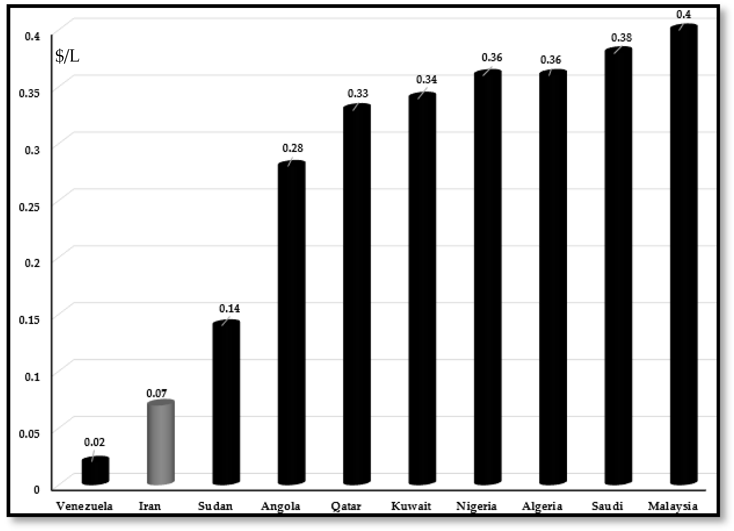
• Low gasoline and diesel prices (Figure 6 and Figure 7) caused by widespread supply of combustible fuels and allocating significant subsidies to them. Based on the report of IEA entitled “World Energy Outlook 2018”, allocating $69 billion for fossil fuels ($26.6 billion, $26 billion, and $16.6 billion for oil, natural gas, and electricity, respectively), Iran ranks as the world’s largest country in terms of allocating fossil fuel consumption subsidies. This amount accounts for 15 percent of total GDP [39].
• The low share of renewable energy in the energy mix and electricity generation [21] despite its high potential.
• The lack of access to advanced renewable technologies, which is caused by imposing sanctions.
• Failure to invest in energy savings and reduce energy intensity due to financial difficulties, which are partially caused by the sanctions.

As it is shown in Figure 6, Iran ($0.07) holds second place in the world in terms of the gasoline price, followed by Venezuela.

As seen in Figure 7, Iran ranks as having the second-lowest diesel price in the world. The low gasoline and diesel prices reduce the private sector’s incentives to invest in alternative energies such as renewable and energy-efficient technologies.

Finally, the response of CO₂ emissions to a positive one standard deviation shock in real GDP is depicted in Figure 8.

According to Figure 8, a positive standard deviation shock to LGDP increases LCO₂ emissions over time. This result could be attributed to the low energy price (as stated before), which increases the energy intensity (Figure 9).

The upward trend of energy intensity shows that over the period, more energy is consumed to produce one unit of output, indicating that higher growth rate emits more carbon dioxide.

To compare the importance of each exogenous innovation (shock) in explaining the forecast error variance of each variable in the same VAR model, the VD was applied. The LCO₂ and LGDP forecast error variance decomposition is illustrated through Figure 10 and Figure 11, respectively.

From Figure 10, on average more than 88.6 percent of forecast error variations in CO₂ emissions were explained by itself. However, the share of renewable electricity in explaining the variation in CO₂ emissions was too small (1.2 percent). This finding confirms the stronger environmental impact of economic growth compared to electricity generation from renewable sources.

Based on Figure 11, LGDP explains the largest proportion of forecast error in its value (on average 71.2 percent), while RES had a lower contribution in explaining the variations in LGDP (9.6 percent).

4. Conclusions and Policy Implication

This study was conducted to evaluate the impact of electricity generation mix on economic growth and CO₂ emissions (as a proxy of environmental degradation) in Iran spanning the period 1980–2016. The SVAR model was applied, and the [30] long-run restrictions were imposed. The result of the inverse roots of VAR characteristics polynomial tests confirmed a well-specified SVAR model.

The impulse response function was conducted to answer the first two research questions. The results demonstrated the positive impact of unit standard deviation shock of renewable electricity to economic growth. Contrary to the expectation, increasing the share of renewable sources in the electricity mix could not reduce carbon dioxide emissions. This finding could be explained by (1) the lack of access to advanced renewable technologies; and (2) the focus of economic and social system of the country’s energy services on development of conventional energies (allocating a huge amount of subsidy) [41,42,43] to keep fossil fuel prices at a low level, which decreased the private sector’s motivations to invest in renewable technologies sources, absence of sustainable energy and environmental policies [22,41,43,44,45,46,47,48,49,50].

The variance decomposition was conducted to answer the fourth research question. The results verified the low share of renewable electricity in explaining forecast error variations in economic growth and CO₂ emissions. Finally, from the empirical findings, increasing the share of renewable energy in generating electricity is not a proper strategy to decrease environmental degradation at this stage of development (the last research question). Therefore, implementing environmental policies such as (1) reviewing and recommending the required amendments to the existing law; (2) increasing environmental regulation especially in the most energy-intensive sectors like power plants and transportation sectors; and (3) implementing robust performance monitoring systems could be the most appropriate policy.

However, providing the required infrastructure to expand renewable energies usage in the next stages of development should be considered by the government and policymakers. For instance, to decrease the dependence on fossil fuels, liberalizing fossil fuel prices and using the money to establish/expand the required renewable sources infrastructures would be an alternative. The required budget could be provided either by creating joint venture agreements or obtaining financial aid and technical support services from international organizations including the Organization of the Petroleum Exporting Countries (OPEC).

References

1. Lin, B.; Zhu, J. The role of renewable energy technological innovation on climate change: Empirical evidence from China. Sci. Total. Environ. 2019, 659, 1505–1512. [Google Scholar] [CrossRef] [PubMed]
2. Sadeghi, A.; Larimian, T. Sustainable electricity generation mix for Iran: A fuzzy analytic network process approach. Sustain. Energy Technol. Assess. 2018, 28, 30–42. [Google Scholar] [CrossRef]
3. Zhixin, Z.; Xin, R. Causal Relationships between Energy Consumption and Economic Growth. Energy Procedia 2011, 5, 2065–2071. [Google Scholar] [CrossRef] [Green Version]
4. Bowden, N.; Payne, J.E. Sectoral Analysis of the Causal Relationship Between Renewable and Non-Renewable Energy Consumption and Real Output in the US. Energy Sources Part B Econ. Plan. Policy 2010, 5, 400–408. [Google Scholar] [CrossRef]
5. Kuznets, S. Economic growth and income inequality. Am. Econ. Rev. 1955, 45, 1–28. [Google Scholar]
6. Grossman, G.; Krueger, A. Environmental Impacts of a North American Free Trade Agreement. Env. Impacts N. Am. Free Trade Agreem. 1991. [Google Scholar] [CrossRef]
7. Shafik, N.; Bandyopadhyay, S. Economic Growth and Environmental Quality: Time-Series and Cross-Country Evidence; World Bank Publications: Washington, DC, USA, 1992; Volume 904. [Google Scholar]
8. Panayotou, T. Empirical Tests and Policy Analysis of Environmental Degradation at Different Stages of Economic Development; International Labour Organization: Geneva, Switzerland, 1993. [Google Scholar]
9. Selden, T.M.; Song, D. Environmental Quality and Development: Is There a Kuznets Curve for Air Pollution Emissions? J. Environ. Econ. Manag. 1994, 27, 147–162. [Google Scholar]
10. Nourry, M. Measuring sustainable development: Some empirical evidence for France from eight alternative indicators. Ecol. Econ. 2008, 67, 441–456. [Google Scholar] [CrossRef]
11. Tiwari, A.K. A structural VAR analysis of renewable energy consumption, real GDP and CO2 emissions: Evidence from India. Econ. Bull. 2011, 31, 1793–1806. [Google Scholar]
12. Silva, S.; Soares, I.; Pinho, C. The Impact of Renewable Energy Sources on Economic Growth and CO2 Emissions: A SVAR approach. Eur. Res. Stud. J. 2012, 15, 133–144. [Google Scholar] [CrossRef] [Green Version]
13. Onafowora, O.A.; Owoye, O. Structural vector auto regression analysis of the dynamic effects of shocks in renewable electricity generation on economic output and carbon dioxide emissions: China, India and Japan. Int. J. Energy Econ. Policy 2015, 5, 1022–1032. [Google Scholar]
14. Al-Mulali, U.; Saboori, B.; Ozturk, I. Investigating the environmental Kuznets curve hypothesis in Vietnam. Energy Policy 2015, 76, 123–131. [Google Scholar] [CrossRef]
15. Al-Mulali, U.; Tang, C.F.; Ozturk, I. Estimating the Environment Kuznets Curve hypothesis: Evidence from Latin America and the Caribbean countries. Renew. Sustain. Energy Rev. 2015, 50, 918–924. [Google Scholar] [CrossRef]
16. Ahmed, K.; Mahalik, M.K.; Shahbaz, M. Dynamics between economic growth, labor, capital and natural resource abundance in Iran: An application of the combined cointegration approach. Resour. Policy 2016, 49, 213–221. [Google Scholar] [CrossRef]
17. Ito, K. CO2 emissions, renewable and non-renewable energy consumption, and economic growth: Evidence from panel data for developing countries. Int. Econ. 2017, 151, 1–6. [Google Scholar] [CrossRef]
18. Pata, U.K. Renewable energy consumption, urbanization, financial development, income and CO2 emissions in Turkey: Testing EKC hypothesis with structural breaks. J. Clean. Prod. 2018, 187, 770–779. [Google Scholar] [CrossRef]
19. Hdom, H.A.D. Examining carbon dioxide emissions, fossil & renewable electricity generation and economic growth: Evidence from a panel of South American countries. Renew. Energy 2019, 139, 186–197. [Google Scholar]
20. Bekun, F.V.; Alola, A.A.; Sarkodie, S.A. Toward a sustainable environment: Nexus between CO2 emissions, resource rent, renewable and nonrenewable energy in 16-EU countries. Sci. Total. Environ. 2019, 657, 1023–1029. [Google Scholar] [CrossRef]
21. Dudley, B. BP Statistical Review of World Energy; BP p.l.c.: London, UK, 2018; Volume 6, Available online: https://www.bp.com/content/dam/bp/business-sites/en/global/corporate/pdfs/energy-economics/statistical-review/bp-stats-review-2018-full-report.pdf (accessed on 8 June 2020).
22. Fadai, D.; Esfandabadi, Z.S.; Abbasi, A. Analyzing the causes of non-development of renewable energy-related industries in Iran. Renew. Sustain. Energy Rev. 2011, 15, 2690–2695. [Google Scholar] [CrossRef]
23. Sims, C.A. Macroeconomics and Reality. Econometrica 1980, 48, 1. [Google Scholar] [CrossRef] [Green Version]
24. Elbourne, A. The UK housing market and the monetary policy transmission mechanism: An SVAR approach. J. Hous. Econ. 2008, 17, 65–87. [Google Scholar] [CrossRef]
25. Bernanke, B.S. Alternative Explanations of the Money-Income Correlation; National Bureau of Economic Research: Cambridge, MA, USA, 1986. [Google Scholar]
26. Blanchard, O.; Watson, M. Are business cycles all alike? In The American Business Cycle: Continuity and Change; University of Chicago Press: Chicago, IL, USA, 1986; pp. 123–180. [Google Scholar]
27. Sims, C.A. Are Forecasting Models Usable for Policy Analysis? Q. Rev. 1986, 10, 2–16. [Google Scholar] [CrossRef]
28. Clarida, R.; Galí, J. Sources of real exchange-rate fluctuations: How important are nominal shocks. In Carnegie-Rochester Conference Series on Public Policy; Elsevier: Amsterdam, The Netherlands, 1994; Volume 41, pp. 1–56. [Google Scholar]
29. Kwiatkowski, D.; Phillips, P.C.; Schmidt, P.; Shin, Y. Testing the null hypothesis of stationarity against the alternative of a unit root. J. Econ. 1992, 54, 159–178. [Google Scholar] [CrossRef]
30. Blanchard, O.J.; Quah, D. The Dynamic Effects of Aggregate Demand and Supply Disturbances; National Bureau of Economic Research: Cambridge, MA, USA, 1988. [Google Scholar]
31. Lütkepohl, H. New Introduction to Multiple Time Series Analysis; Springer: Berlin/Heidelberg, Germany, 2005. [Google Scholar]
32. Amisano, G.; Giannini, C. From var models to structural var models. In Topics in Structural VAR Econometrics; Springer: Berlin/Heidelberg, Germany, 1997; pp. 1–28. [Google Scholar]
33. Lütkepohl, H. Estimation of structural vector autoregressive modelsCommun. Stat. Appl. Methods 2017, 24, 421–441. [Google Scholar]
34. Kilian, L.; Lütkepohl, H. Structural Vector Autoregressive Analysis; Cambridge University Press: Cambridge, MA, USA, 2017. [Google Scholar]
35. World Bank Open Data. Available online: http://data.worldbank.org/indicator (accessed on 8 June 2020).
36. U.S. Energy Information Administration. Available online: https://www.eia.gov/beta/international/analysis (accessed on 8 June 2020).
37. Tiwari, A.K. Globalization and wage inequality: A revisit of empirical evidences with new approach. J. Asian Bus. Manag. 2010, 2, 173–187. [Google Scholar]
38. Maslyuk, S.; Dharmaratna, D. Renewable Electricity Generation, CO2 Emissions and Economic Growth: Evidence from Middle-Income Countries in Asia. Stud. Appl. Econ. 2020, 31, 217–244. [Google Scholar] [CrossRef]
39. International Energy Agency. IEA World Energy Outlook; IEA OECD: Paris, France, 2018. [Google Scholar]
40. Global Petrol Price. Available online: www.Globalpetrolprices.Com (accessed on 13 July 2020).
41. Mirza, U.K.; Ahmad, N.; Harijan, K.; Majeed, T. Identifying and addressing barriers to renewable energy development in Pakistan. Renew. Sustain. Energy Rev. 2009, 13, 927–931. [Google Scholar] [CrossRef]
42. Pegels, A. Renewable energy in South Africa: Potentials, barriers and options for support. Energy Policy 2010, 38, 4945–4954. [Google Scholar] [CrossRef]
43. Rezaee, M.J.; Yousefi, S.; Hayati, J. Root barriers management in development of renewable energy resources in Iran: An interpretative structural modeling approach. Energy Policy 2019, 129, 292–306. [Google Scholar] [CrossRef]
44. Bezir, N.Ç.; Murat, Ö.; Nuri, Ö. Renewable energy market conditions and barriers in Turkey. Renew. Sustain. Energy Rev. 2009, 13, 1428–1436. [Google Scholar]
45. Ansari, F.; Kharb, R.K.; Luthra, S.; Shimmi, S.; Chatterji, S. Analysis of barriers to implement solar power installations in India using interpretive structural modeling technique. Renew. Sustain. Energy Rev. 2013, 27, 163–174. [Google Scholar] [CrossRef]
46. Eleftheriadis, I.M.; Anagnostopoulou, E. Identifying barriers in the diffusion of renewable energy sources. Energy Policy 2015, 80, 153–164. [Google Scholar] [CrossRef]
47. Luthra, S.; Kumar, S.; Garg, D.; Haleem, A. Barriers to renewable/sustainable energy technologies adoption: Indian perspective. Renew. Sustain. Energy Rev. 2015, 41, 762–776. [Google Scholar] [CrossRef]
48. Ghimire, L.P.; Kim, Y.; Kim, Y. An analysis on barriers to renewable energy development in the context of Nepal using AHP. Renew. Energy 2018, 129, 446–456. [Google Scholar] [CrossRef]
49. Shah, S.A.A.; Solangi, Y.A.; Ikram, M. Analysis of barriers to the adoption of cleaner energy technologies in Pakistan using Modified Delphi and Fuzzy Analytical Hierarchy Process. J. Clean. Prod. 2019, 235, 1037–1050. [Google Scholar] [CrossRef]
50. Asante, D.; He, Z.; Adjei, N.O.; Asante, B. Exploring the barriers to renewable energy adoption utilising MULTIMOORA- EDAS method. Energy Policy 2020, 142, 111479. [Google Scholar] [CrossRef]
Figure 1. Conceptual framework.
Energies 13 04268 g001
Figure 2. Long-run restrictions.
Energies 13 04268 g002
Figure 3. Stability of Vector Autoregressive Model.
Energies 13 04268 g003
Figure 4. Response of LGDP to RES using structural VAR factor.
Energies 13 04268 g004
Figure 5. Response of LCO2 to RES using structural VAR factor.
Energies 13 04268 g005
Figure 6. Top ten world’s lowest gasoline price 13 July 2020 [40].
Energies 13 04268 g006
Figure 7. Top ten world’s lowest diesel price 13 July 2020 [40].
Energies 13 04268 g007
Figure 8. Response of LCO2 to LGDP using structural VAR factor.
Energies 13 04268 g008
Figure 9. Energy intensity level of primary energy [35].
Energies 13 04268 g009
Figure 10. LCO2 forecast error variance decomposition results.
Energies 13 04268 g010
Figure 11. LGDP forecast error variance decomposition results.
Energies 13 04268 g011