Development of an Elevation–Fresnel Linked Mini-Heliostat Array

Abstract

Heliostats are critical components of solar tower technology and different strategies have been proposed to reduce their costs; among them diminishing their size to reduce wind loads or linking nearby heliostats mechanically, to reduce the overall number of actuators. This document aims to describe the development of a linked array of mini-heliostats which move together in an elevation–Fresnel configuration. This configuration consists of an array of mirrors rotating around linked parallel axes, in a linear Fresnel style with an added elevation mechanism allowing all axes to incline simultaneously in the plane North–South–Zenith; that is equivalent to an array of N linked mini-heliostats moved by only two drives instead of 2N. A detailed analytical study of the Sun-tracking performance of this kind of heliostat arrays was carried out, and an 8-mirror prototype based on optical and mechanical analyses was designed, built and tested. Even though the mirrors are flat, the array produced a rather compact radiative flux distribution on the receiver. The flux distribution is compatible with a slope error of the order of 1 mrad. Peak and mean concentration ratios reached 6.89 and 3.94, respectively.

1. Introduction

Solar tower power plants [1,2,3,4] are the second most widely extended solar thermal technology for electricity generation, with more than 20 commercial projects operating in the world. Heliostats are critical components of this technology. The heliostat field is the most expensive component in the power plant [4,5,6], up to 60% of the overall capital cost. Therefore, the development of improved heliostat technology has been one of the research foci in recent years. Engineers have devised different development strategies to cope with the challenge of making a more affordable technology [7,8,9]. One of these strategies consists of reducing the size of heliostats [10], thus departing from the main historical path of the technology towards large heliostats [11]. Another one is the use of high-density heliostat fields, where these small heliostats are closer to each other than usual shadowing and blocking considerations dictate [12].

Heliostats are long focal distance point focus mirrors, used to concentrate solar radiation on a fixed receiver. They usually have two drives, consisting of motors coupled with mechanical reduction gearboxes, to produce the two independent rotations necessary for tracking the Sun’s apparent movement in the sky. Thus, many tracking mechanisms are required for heliostat fields consisting of hundreds or thousands of heliostats. This circumstance-oriented development of heliostats towards increased size [11] to reduce the number of costly, high-precision, mechanical components and controllers required per unit mirror area. In the last 15 years, this paradigm has been questioned, and currently there is no consensus on the optimal size of heliostats [8,9].

Small-size heliostats have much less stringent requirements with wind loads and torque so the alternative development path follows the way of reducing the size of these units, based on that much cheaper drives can be employed [10] and electronic control components have become much less expensive in recent decades [13].

Another direction of research is the reduction of control units by way of linking nearby heliostats mechanically, to reduce the overall number of actuators [6,14,15,16]. This approach logic is that small heliostats require quite similar movements due to their proximity. The coupled movement of mini-heliostats implies leaving aside the typical azimuth-elevation tracking mechanism. For instance, a concept proposed by Göttsche et al. [6] consist of very small mirrors (10 × 10 cm) mounted on ball-in-socket joints driven by a stepper motor. Dunham et al. [14] analyzed the effect of linking heliostats in different numbers, when they are distributed on a square mesh over a flat land surface. They calculated the monthly energy efficiency of the coupled heliostats as compared to independent tracking units. Amsbeck et al. [15] presented a study on the concept of torque tube heliostat, where a group of mini-heliostats are fixed into a common long torque tube for elevation movement. They considered the yearly behavior of a torque tube heliostat field and compared it to a conventional field and found only 3% reduction in the annual energy yield. More recently, a tensile coupled heliostat prototype has been evaluated [16] by Sandia National Labs group, consisting of a row of mini-heliostats suspended by two cables. In all cases, as a consequence of this coupled movement, individual heliostat aiming becomes less accurate. Ideally, this reduction should be compensated by potential savings arising from the reduction in drive units.

Recently, a collaboration between IER-UNAM (UNAM’s Institute of Renewable Energies) and the private company Gadgets & Design S.A. de C.V., Mexico City, Mexico, started. We were awarded a one-year grant in the framework of PRODETES international award Mexico (Sustainable energy technology development project, by its Spanish acronym; funded by the Global Environmental Facility GEF of the World Bank). The aim of the project is to carry out the development of solar tower technology for high temperature industrial heat. This document describes the development of a linked array of mini-heliostats within this project. These heliostats move together in an elevation–Fresnel configuration as illustrated in Figure 1. The configuration consists of an array of mirrors that rotate around linked parallel axes, like a linear Fresnel reflector [17], but with an added elevation mechanism that inclines all those axes simultaneously in the North–South–Zenith plane. Thus, the arrangement of N facets is equivalent to N linked mini-heliostats moved by only two drives instead of $2N$. In particular, an eight-facet unit was built and tested with satisfactory results. Optical tests were carried out, where the radiative flux distribution, peak and average concentration ratios produced by the heliostat were evaluated and compared with ray tracing analysis. Additionally, this document examines the elevation–Fresnel tracking in detail and discusses the associated accuracy loss and its causes.

2. Methodology

2.1. Theoretical Model

In the tracking configuration described before the angles of the central mini-heliostat govern the global tracking of the array. For an array with an even number of mini-heliostat units, this central heliostat does not exist. In such a case, the tracking angles correspond to an imaginary heliostat located at the center of the array. Therefore, the central facet tracks the sun at the correct angles, and the rest of the mini-heliostats follow suit. The actual rotation angle of each facet (Figure 2) is related to the angle of the central facet as

$${\psi }_j\left(t\right)={\psi }_0\left(t\right)+\Delta {\psi }_j,$$

(1)

where ${\psi }_j\left(t\right)$ and ${\psi }_0\left(t\right)$ are the angles of facets j and 0, respectively, and $\Delta {\psi }_j$ is the constant rotation offset of the j facet to the 0 facet; i.e., the canting angle [18]. From the above equation, angular speeds are identical for all mini-heliostats, i.e.,

$$\frac{d{\psi }_j}{dt}=\frac{d{\psi }_0}{dt}=\mu \left(t\right).$$

(2)

The offsets $\Delta {\psi }_j$ are such that all the units aim solar rays at the desired focal point for a chosen canting day at noon. On the other hand, all facet rotation axes have the same inclination

$${\xi }_j\left(t\right)={\xi }_0\left(t\right)=\xi \left(t\right).$$

(3)

The objective of the proposed tracking mode is to couple several small heliostats with only two actuators, one of them to provide the elevation $\xi$ and a second one for the joint rotation at $\mu$ speed. Of course, the aiming of each heliostat loses accuracy.

Calculating the light reflection by the heliostats of the array requires first to determine the central facet angles. Figure 3a shows a global reference system where $\widehat{\mathbf{s}}$ is the unit vector pointing to the Sun, $\widehat{\mathbf{n}}$ is the unit vector of the normal to the reflector surface, and $\widehat{\mathbf{t}}$ is the reflected unit vector pointing to the target R at the receiver. The origin is at the heliostat center, and the tower locates to the South.

For a given location and time, if the solar vector $\widehat{\mathbf{s}}$ is known and the relative target location $\widehat{\mathbf{t}}$ unit vector is fixed, the central facet should be oriented such that the reflection law is satisfied;

$$\widehat{\mathbf{n}}=\frac{\widehat{\mathbf{s}}+\widehat{\mathbf{t}}}{∥\widehat{\mathbf{s}}+\widehat{\mathbf{t}}∥}.$$

(4)

Here we take $\widehat{\mathbf{n}}={\widehat{\mathbf{n}}}_0$ and $\widehat{\mathbf{t}}={\widehat{\mathbf{t}}}_0$, the vectors corresponding to the central facet.

To orient the central facet with the elevation–Fresnel mechanism, it is necessary to rotate the ${\xi }_0$ and ${\psi }_0$ angles as shown in the Figure 3b: first a rotation by an angle ${\xi }_0$ around the x axis in the $\pi$ plane ($yz$ plane), followed by a second rotation by the ${\psi }_0$ angle around the axis $y^{\prime }$ in the ${\pi }^{\prime }$ plane (${\widehat{n}}^{\prime }x$ plane). Thus, in the global $xyz$ reference system of Figure 3a, the normal vector in terms of these angles is

$${\widehat{\mathbf{n}}}_0=(sin{\psi }_0,-cos{\psi }_{0}sin{\xi }_0,cos{\psi }_{0}cos{\xi }_0).$$

(5)

From this equation, the components of the normal vector ${\widehat{\mathbf{n}}}_0=(n_{0x},n_{0y},n_{0z})$ are related to the angles ${\xi }_0$ and ${\psi }_0$ by

$${\psi }_0=arcsin\left(n_{0x}\right),$$

(6)

and

$${\xi }_0=arccos\left(\frac{n_{0z}}{cos{\psi }_0}\right).$$

(7)

With the previous analysis, the required tracking angles of the central facet ${\psi }_0$ and ${\xi }_0$ are calculated as a function of time, according to the required evolution of the normal vector, predicted by Equation (4). It only remains to determine the necessary canting angles of the lateral mini-heliostats $\Delta {\psi }_j$.

There are different canting methods for heliostats [18]. In the present case canting is done by choosing a canting day, and demanding that the central rays from all mini-heliostats hit the center of the target at solar noon. It is always possible to achieve this in the horizontal direction by adjusting the $\Delta {\psi }_j$ angles only, because the system becomes equivalent to a linear concentrator at that time of the day. In the vertical direction a small difference persists in the impact points from different facets, as we will see in Section 3.1, because the ${\xi }_j$ angles cannot be independently adjusted. Thus, once the angle ${\psi }_0$ is fixed, the canting angles $\Delta {\psi }_j$ are obtained by demanding that Equation (4) is fulfilled in the x direction, at noon, for this particular day, for all the mini-heliostats. Analogously with Equation (6), we can obtain    

$$\Delta {\psi }_j=arcsin\left(n_{jx,\mathrm{noon}}\right).$$

(8)

Once the array is canted, the tracking can be simulated. This is done by continuously varying the solar vector $\widehat{\mathbf{s}}\left(t\right)$, according to the Sun position equations [19], and obtaining the tracking angles of the central facet from Equations (4), (6) and (7). Then the ${\psi }_j$ angles of the rest of the mini-heliostats are obtained from Equation (1), and their normal vectors from Equation (5).

To evaluate the quality of the tracking, we calculate the reflected vectors from the center of each facet and determine the impact points on the target. The reflected vector for the j facet, ${\widehat{\mathbf{r}}}_j$, is obtained by

$${\widehat{\mathbf{r}}}_j=2(\widehat{\mathbf{s}}·{\widehat{\mathbf{n}}}_j){\widehat{\mathbf{n}}}_j-\widehat{\mathbf{s}}.$$

(9)

The impact point on the target ${\mathbf{T}}_j$ is obtained as

$${\mathbf{T}}_j={\mathbf{f}}_j+D_j{\widehat{\mathbf{r}}}_j;$$

(10)

where ${\mathbf{f}}_j$ is the position of facet j, and $D_j$ is the distance to the impact point. For a flat receiver with an orientation given by the normal unit vector ${\widehat{\mathbf{n}}}_p$ and location provided by its center coordinate $\mathbf{R}$, this distance is given by

$$D_j={\displaystyle \frac{{\widehat{\mathbf{n}}}_p·(\mathbf{R}-{\mathbf{f}}_j)}{{\widehat{\mathbf{n}}}_p·{\widehat{\mathbf{r}}}_j}}.$$

(11)

By combining Equations (10) and (11), the impact point ${\mathbf{T}}_j$ in the receiver for the ray reflected at the center of facet j can be determined.

Finally, the effect of the elevation–Fresnel tracking over the concentrated radiative flux distributions is studied. To this end, a script LK [20] was written to use the SolTrace software [21]. A program in C was developed for the calculation of the solar $\widehat{\mathbf{s}}$ and normal vectors ${\widehat{\mathbf{n}}}_j$ of the mini-heliostats, used as inputs for SolTrace.

As input value for the Direct Normal Irradiance (DNI) at different times and days, values obtained from a clear sky model [14] were used:

$$G_b=G_0{\tau }^{m^{0.678}},$$

(12)

where $G_0$ is Solar Constant of $1367\mathrm{W}/{\mathrm{m}}^2$, $\tau$ is the atmospheric transmittance, assumed as 0.7 under clear sky conditions. The air mass m is given by

$$m=\frac{exp(-0.0001184h_{\mathrm{alt}})}{cos{\theta }_z+0.5057{(96.080-{\theta }_z)}^{-1.634}},$$

(13)

where $h_{\mathrm{alt}}$ is the altitude with respect to sea level, and ${\theta }_z$ is the solar zenith angle.

The simulations considered a Gaussian Sun shape with 2.73 mrad standard deviation, and the concentrator optical properties used were: reflectivity 1.0, slope error 2.64 mrad, and 0.1 mrad specularity error. The mesh on the receiver was of $50\times 50$ bins. To evaluate the number of rays required, a preliminary set of simulations for an array of eight mini-heliostats was carried out by using from $5\times {10}^3$ to $7\times {10}^6$ rays. The total power on the receiver stabilized for $4\times {10}^6$ rays, with an error of 0.08% as compared to $7\times {10}^6$ rays. Therefore, for the rest of the simulations, $5\times {10}^6$ rays were used.

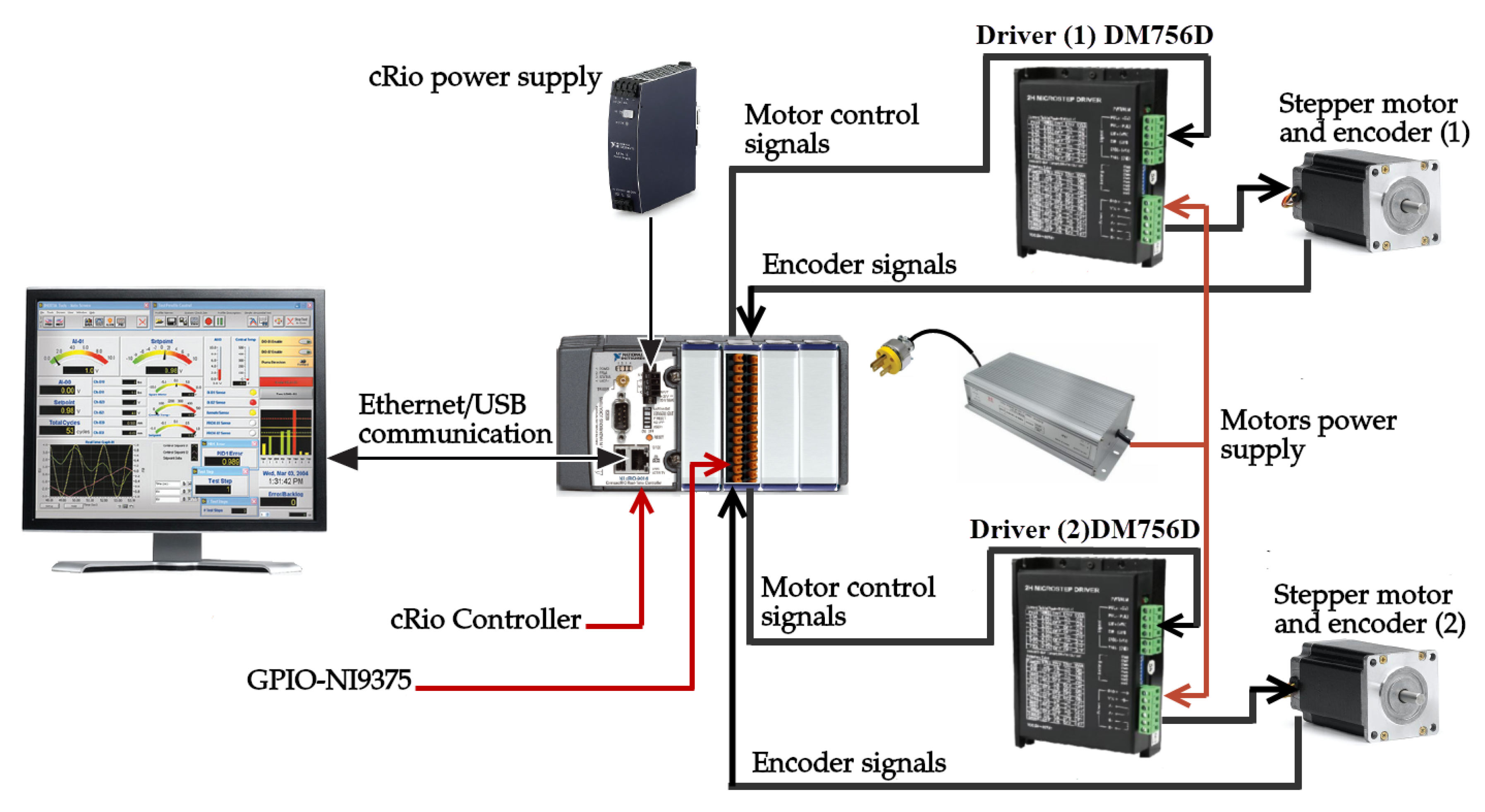
2.2. Experimental Methods

Different experiments were performed for the characterization of the linked heliostat array prototype. The specular reflectivity of the array mirrors, as a function of wavelength ${\rho }_{\lambda }$, was measured using a JASCO UV-Vis-NIR spectrophotometer, model V-670. Measurements were carried out in the interval from 250 to 2500 nm, with 2 nm step, using a first surface Aluminum mirror as a reference. With this data, the solar reflectance ${\rho }_s$ of the array mirrors was evaluated by considering the ASTM G173-03 beam solar irradiance spectrum, which corresponds to Air Mass 1.5 and DNI of $G_b=899.55\mathrm{W}/{\mathrm{m}}^2$. In terms of the spectral irradiance $G_{\lambda }$, the solar specular reflectance is given by

$${\rho }_s=\left({\int }_{250}^{2500}{\rho }_{\lambda }{G}_{b,\lambda }d\lambda \right){\left({\int }_{250}^{2500}{G}_{b,\lambda }d\lambda \right)}^{-1}$$

(14)

The radiative flux distribution produced by the mini-heliostat array was characterized by projection onto a $2.44\mathrm{m}\times 2.44\mathrm{m}$ target, located at the roof of a building, 37 m South from the solar platform, at 4.635 m height, relative to the array center. A water-cooled heat-flux sensor, located at the center of the target, was used to measure the concentrated solar radiative flux. The sensor, type Gardon, model SBG01-TCK-050 from Hukseflux, has a rated measurement up to $50\mathrm{kW}/{\mathrm{m}}^2$. The direct-current voltage output from this sensor was measured with a Keysight data acquisitor model DAQ970A, and transformed to radiative flux by using the sensitivity constant

$$S=0.256\times {10}^{-6}\frac{\mathrm{V}}{\mathrm{W}/{\mathrm{m}}^2}$$

(15)

A CMOS camera model Mako U-130 from Allied Vision was used to take photographs of the radiative flux distribution. This camera has a resolution of $1280\times 1024$ pixels and a sensor size of $6.4\mathrm{mm}\times 4.8\mathrm{mm}$, with 8-bit dynamic range. The camera used a lens of 100 mm focal length, model SV-10028H from VS Technology Corporation, which has a maximum aperture ratio of 1:2.8. To reduce light intensity without affecting color and contrast, neutral density filters were used, model NI120-37.5 from MIDOPT, which have an optical density of 1.2 and 6.25% transmittance. From the camera, lens, and target data, a resolution of $0.244\mathrm{cm}\times 0.229\mathrm{cm}/\mathrm{pixel}$ was determined on the target. The intensity values of the images captured by the camera were converted from grayscale to irradiance values by calibration with the measurements obtained from the Gardon heat-flux sensor [22].

Before testing, the array was aligned to the East-West axis and leveled with a self-leveling cross and line laser, model Lino L2P5 from Leica. The working range is up to 25 m and it automatically adjusts its positioning up to $\pm 4^{\circ }$ when out of level. The heliostats of the array were canted to the angular offsets corresponding to March 21st, at solar noon. This operation was done with the help of digital inclinometers, model HPS-60-2-235 96332 from Level developments, with a precision of ${0.002}^{\circ }$, in the range of $\pm {60}^{\circ }$. The canting angle of each mirror was measured at its center. Once the canting operation had been realized, an estimation of the slope error for each facet was done by measuring the angle differences between different points in the mirror relative to the center.

The coordinates of the center of the target, the center of the mini-heliostat array, and the camera, were determined as $(0.0,0.0,5.811)$, $(-3.738,38.608,1.176)$, and $(-1.038,48.957,0.011)$ m, respectively. The origin of the reference system considered was at ground level, just below the target, with the x axis pointing West, y North, and z to the Zenith. From this data, the line of sight distance from the array to the target was 39.064 m. Please note that the horizontal projection of the line connecting the array and target centers is not parallel with the North–South axis.

Finally, Direct Normal Irradiance (DNI) was measured with an Eppley pyrheliometer, model NIP, every 15 s. The direct-current voltage output from this instrument is converted to radiative flux by using the sensitivity constant

$$k=107.3\frac{\mathrm{W}/{\mathrm{m}}^2}{\mathrm{mV}}$$

(16)

3. Results

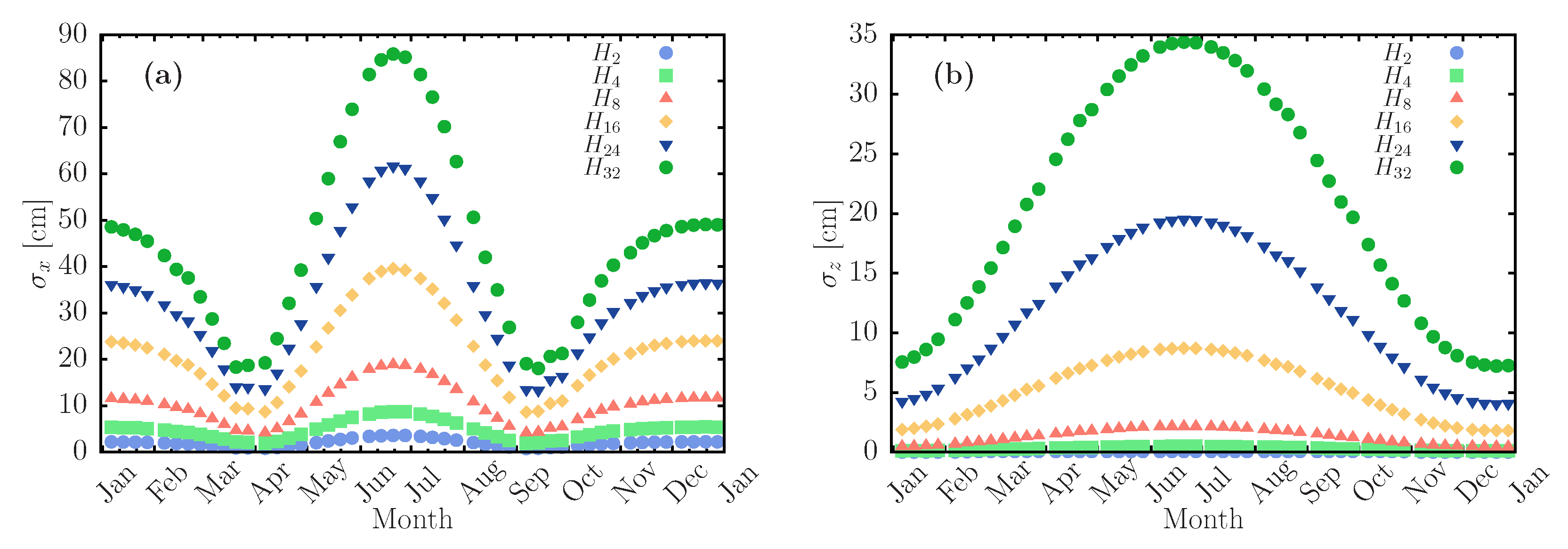
3.1. Theoretical Analysis

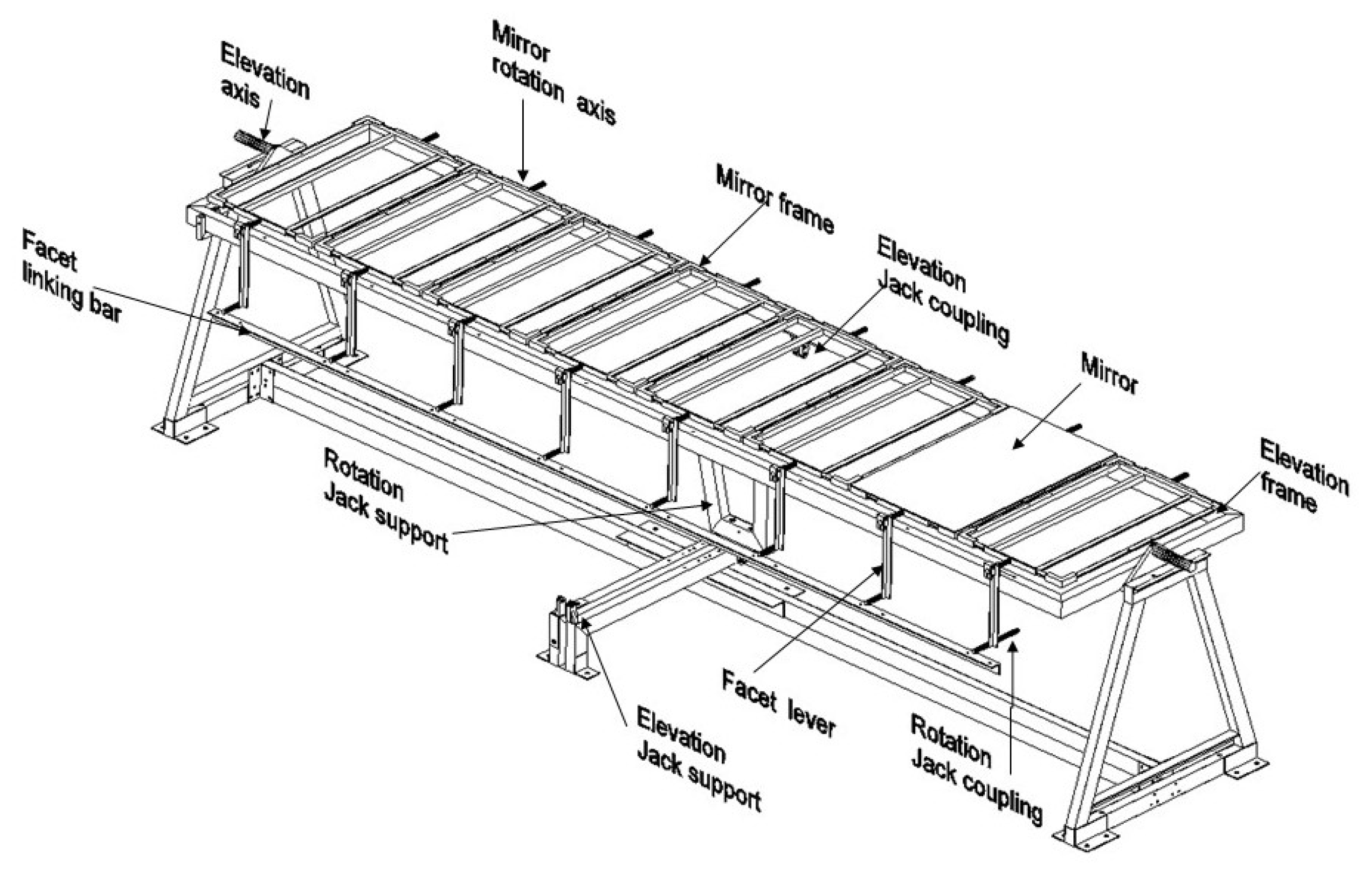
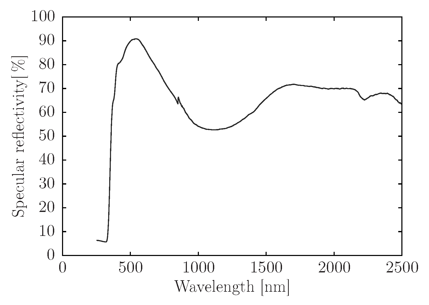
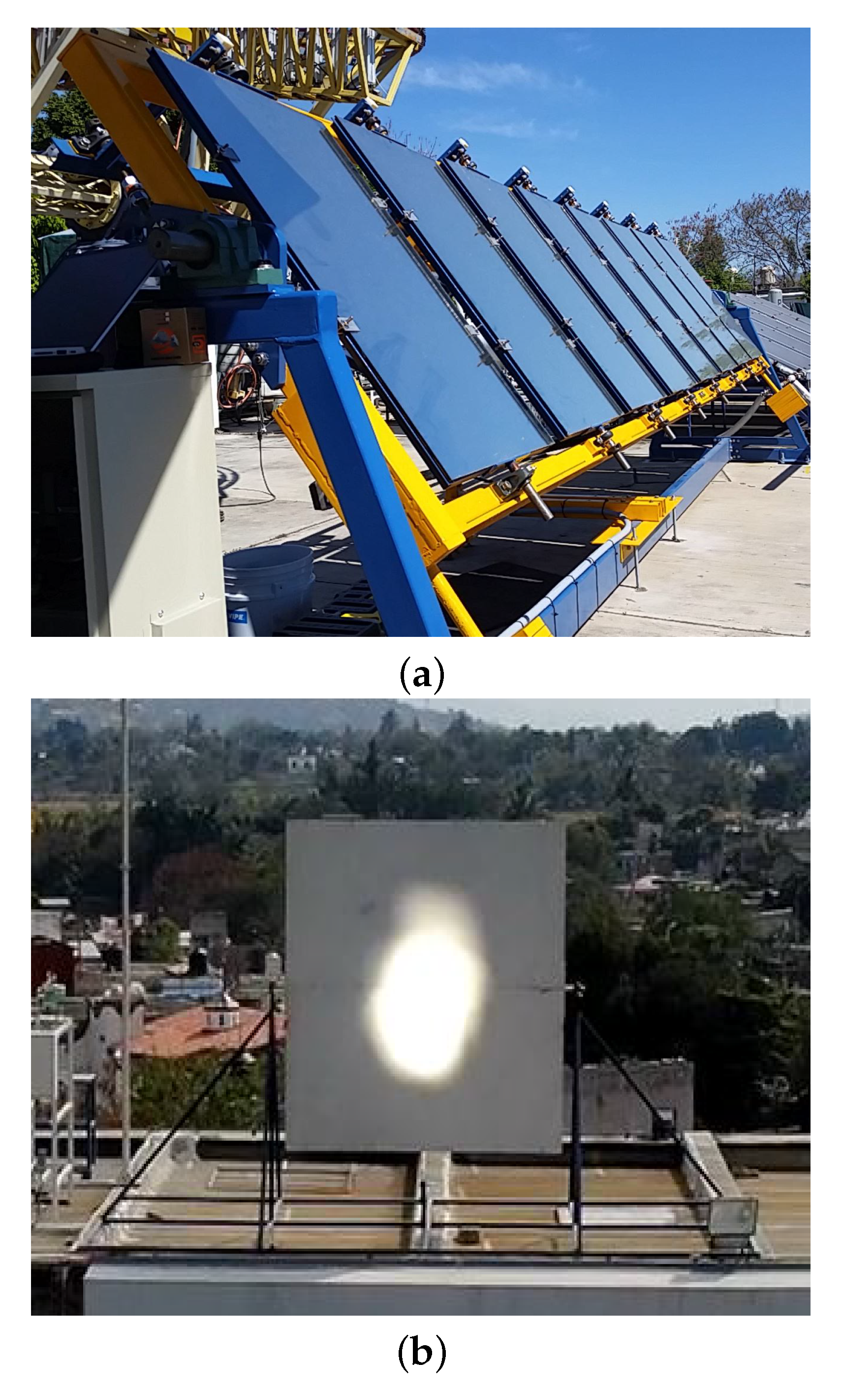
With the methodology described in Section 2.1, arrays consisting of 2, 4, 8, 16, and 32 mini-heliostats (identified as H2, H4, H8, H16, and H32, respectively) were simulated. Also, a single facet heliostat (H1) was included in some cases for comparison. Please note that the latter is equivalent to an ordinary heliostat for the present purposes. Each facet has the dimension of $1\mathrm{m}\times 1\mathrm{m}$, and a gap of 20 cm exists between them. All the presented results were obtained for arrays canted on the equinox. In previous analyses [23], this canting day was shown to produce the smallest yearly spread of impact points, so this point will not be further discussed here.

The location considered for the present simulations is Hermosillo, Mexico, located at ${29.028452}^{\circ }$ +N latitude, ${111.145475}^{\circ }$ +O longitude, and 200 m altitude, unless otherwise indicated. The simulation results are reported in solar time, starting one hour after sunrise (−${\omega }_a+{15}^{\circ }$) and finishing one hour before sunset (${\omega }_a-{15}^{\circ }$). The receiver was placed at a height $h=35$ m. The heliostat array was located to the North of the tower, at three different distances along the y axis (expressed as multiples of the tower height): $0.75h$ (26.25 m), $2h$ (70 m), and $4h$ (140 m).

As a first example, consider the H4 array. Figure 4 shows the impact points of the central ray from each mini-heliostat on the target ($xz$ plane). Points correspond to every hour, from 7:30 h to 16:30 h, on 21 March. Due to the symmetry of the Sun’s apparent trajectory and the tracking mechanism, the facets’ impact point trajectories reverse direction at noon, and go back on their steps, to end at the initial point. Figure 4a,b show the behavior for heliostat locations at 0.75h and 2h, respectively. Please note that the z axis scale remains the same in both figures, while the x axis scale is much larger for the second case. The number of time intervals considered is five, one for each hour from 7:30 to 11:30, as corresponding points in the afternoon are identical. However, the points closer to noon tend to overlap and they cannot be visually separated from each other. For instance, in Figure 4a, for facets 1 and 2 one can only distinguish the point corresponding to 7:30, while the others overlap at the center.

Please note that even though the results presented in Figure 4a correspond to the canting day, not all reflected rays hit the target center at noon, because all mini-heliostats share the same elevation $\xi$. The present tracking scheme only guarantees that all the reflected rays fall on the central vertical axis of the target at noon for the canting day. However, note also that the vertical deviations are quite small. The difference between ideal and actual value of the angle ${\xi }_j$ increases with the distance of the facet j to the center of the array. For example, the differences are 0.028, 0.704, and 2.821 mrad, for the outermost facets of H4, H16, and H32 arrays, respectively, when located at $0.75h$.

Figure 5 presents the behavior of impact points for the 21st day of each month, from June to December (note that the annual behavior is symmetrical around June). It is interesting to observe how the impact points of symmetric heliostat pairs switch sides throughout the year. The minimum dispersion occurs on the day of canting, 21 March/September, where the solar declination is zero. The maximum dispersion occurs in June. Values of 11.8, 15.1, and 19.6 cm, on the x axis, and −2.1, −1.1, and −0.6 cm, on the z axis, are obtained for the positions 0.75h, 2h, and 4h, respectively.

In the following graphs, to present results for a whole year, we calculate the daily standard deviation, which characterizes the spread of all mini-heliostats’ impact points. These are represented as ${\sigma }_x$ and ${\sigma }_z$, for the x and z directions, respectively. Figure 6 shows the behavior of the daily standard deviations throughout the year, for array H4 located at 0.75h, 2h, and 4h. An increase in the standard deviation with distance occurs on the x axis (Figure 6a), while the opposite happens (Figure 6b) along z axis.

The number of mini-heliostats in the array affect the distribution of impact points on the receiver. Figure 7 shows the daily standard deviations for all heliostat arrays, when located at 2h. The deviations increase with the number of mini-heliostats, reaching their maximum values for 21 June. The error increases proportionally to the number of mini-heliostats on the array, which makes sense, since the lateral size of the array is proportional to this parameter.

Ray tracing simulations were carried out to evaluate the solar radiation concentration and energy collection performance of all the considered arrays. The receiver has a $6\times 6{\mathrm{m}}^2$ area. Figure 8 shows the radiative flux distribution for the H8 array, at a position of 0.75h, for June and 21 December, at solar noon. The shape of both graphs looks similar, but radiative flux is more spread for the second case. Peak flux changes from 4.054 to 3.573 kW/m${}^2$ between June and December. The power on the receiver has values of 7400 W for June and 6574 W for December. This is an 11.16% diminution due to lower DNI.

Figure 9 shows the radiative flux distribution for H32, for 21 June, which is the case with the highest radiative flux dispersion. The peak flux at 6:30 h is 2.978 kW/m${}^2$, which increases to 5.242 kW/m${}^2$ at 9:30 h and remains unchanged until solar noon. This spread of the concentrated solar flux in June limits the concentration, compared to other months, i.e., 21 January, where a more compact distribution is obtained at solar noon, with a peak flux of 9.609 kW/m${}^2$ (similar in shape to Figure 8a, but not shown here for reasons of space).

Previous graphs showed the energy contained in a receiver of $6\mathrm{m}\times 6\mathrm{m}$ with around 99% of the energy. The radiative flux distribution standard deviations along x and z axis, namely $S_x$ and $S_z$, give a more accurate idea of the variation of the size of this distribution.

Figure 10 shows the average daily standard deviations ${\overline{S}}_x$ and ${\overline{S}}_z$, for arrays placed at a distance of 2h. For arrays of 2, 4, 8, and 16 mini-heliostats, these daily deviations have only small variation throughout the year. However, for the 24 and 32 mirror arrays, the deviations in the x axis increase strongly for January, May, June, July, November, and December. In contrast, in the z axis the highest values appear for March, April, August, and September. The average deviations throughout the year for an H2 array are ${\overline{S}}_x=0.766\pm 0.015$ and ${\overline{S}}_z=0.840\pm 0.038$, while for an H8 array the corresponding values are $0.777\pm 0.016$ and $0.835\pm 0.054$, respectively.

The choice between flat or concentrating mirrors is another relevant aspect to analyze for the development of mini-heliostat arrays. This comparison is addressed in Figure 11, where two arrays of eight mirrors with 0.6 m width and 1 m height are compared. Spherical curvature is considered for concentrating facets, with a focal length equal to the slant range. The receiver was placed at a height $h=8$ m and the heliostat array located at distances of 37 m. Figure 11 shows the daily standard deviations of impact points on the target in the vertical and horizontal directions. The flat mirror array has standard deviations of ${\overline{S}}_x=0.435$ and ${\overline{S}}_z=0.448$ m, while the use of concentrating facets reduces those values to ${\overline{S}}_{xc}=0.367$ and ${\overline{S}}_{zc}=0.316$ m. Figure 11b shows the variation of the peak concentrated radiative flux through the year for the two arrays. The peak flux is more than doubled on the average when concentrating mirrors are used.

Based on the radiative flux distributions obtained, the daily energy incident on the receiver was calculated for the 21st of each month, for arrays placed at 0.75h. The results are shown in Figure 12, where an H1 array, energetically equivalent to a single heliostat with a zenith-azimuth tracking, is also presented for reference. The graph shows the contribution of daily energy per mini-heliostat, i.e., the total energy supplied, divided by the number N of mini-heliostats of the array. As expected, due to the imperfect tracking, the energy per mirror decreases with N. However, the graph shows that the maximum decay is always between H1 and H2, and becomes less significant as the array size increases. The annual average reduction between the H1 and H2 arrays is 4.4%, between H2 and H4 is 2.3%, between H4 and H8 is 1.21%, between H8 and H16 is 0.72%, between H16 and H24 is 0.39%, and between H24 and H32 is 0.38%. The trend is that the energy per facet for arrays larger than H32 will have little variation, although the shape of the concentrated solar flux distribution becomes irregular, as seen in Figure 9.

Looking again at Figure 7, we have the maximum standard deviation in June, yet December is the month with the lowest energy (Figure 12), mainly because of the number of daylight hours.

3.2. Prototype

Based on the theoretical analysis, it was decided to design and build a prototype array of eight linked mini-heliostats for demonstrating all the concept features, with a manageable size unit and keeping tracking errors small.

The mainly evaluated factors for the mechanical design, both in normal operation conditions and in the safety stowage position, were loads due to wind. In service, up to 22 m/s wind speed, it was necessary to ensure that the actuators could overcome the torque around different axes and the structure’s bending due to these loads should not undermine the system optical performance. In the stow position, the array should survive wind speeds up to 48 m/s.

Structural analysis was used to select materials and dimensions that ensure satisfactory operation under the conditions described above, according to maximum stress and deformations. The analysis was performed for the elevation frame and the support element. An additional $10\%$ of mass load and $10\%$ of wind load were considered, in both positions. As the maximum stress of the array elements is less than the yield strength of the steel (250 MPa), survival is guaranteed. Also, maximum angular deformations are were limited to 1 mrad, to avoid affecting the system optical performance. This criterion implied, for instance, a maximum tolerance of 2 mm deformation for the longest beams in the frame supporting the individual heliostat rotation axes. Figure 13 shows an image of the resulting structure. Also,

Table 1. Main characteristics of the prototype.

Parameter	Value	Units
Number of facets	8	–
Facet length	1.00	m
Facet width	0.60	m
Mirror material	Back silvered glass	–
Mirror thickness	6	mm
Structure material	ASTM A36 Steel	–
Spacing between facets	0.02	m
Length of the elevation frame	5.062	m
Width of the elevation frame	1.13	m
Height of the array	1.6	m
Type of actuator	Linear jack /stepper motor	–
Elevation range	[5, 80]	deg
Facet rotation range	[−53.71, 53.71]	deg

gives the main geometric characteristics and materials of this array.

As shown in Table 1, back silvered glass mirrors with 6 mm thickness were used in the array. The spectral specular reflectivity of this mirror of Vitro brand is shown in Figure 14. The reflectivity deteriorates significantly in the infrared region (above 720 nm). It is not clear if the cause of this behavior is absorption by the glass or low reflectivity of the silver film, but this is low even compared to 6 mm mirrors from other brands. A value of $72.48\%$ was obtained for the broadband solar reflectance ${\rho }_s$, by using Equation (14). A photograph of the prototype is shown in Figure 15.

From the theoretical analysis (Section 3.1), the best canting for the array corresponds to the solstices. Thus, the angles of the facets were calculated for March 21st, as listed in

Table 2. Canting angle of the mirrors corresponding to 21st March, at solar noon, and slope errors.

Facet	${\mathit{f}}_8$	${\mathit{f}}_6$	${\mathit{f}}_4$	${\mathit{f}}_2$	${\mathit{f}}_1$	${\mathit{f}}_3$	${\mathit{f}}_5$	${\mathit{f}}_7$
Canting angle (deg)	1.884	1.346	0.808	0.269	−0.269	−0.808	−1.346	−1.884
Slope error (mrad)	1.36	0.75	1.41	1.68	0.87	1.26	1.32	0.77

. As explained in Section 2.2, an estimation of slope errors was obtained from measurements at different points of the facets. The obtained values are also shown in Table 2.

The instantaneous movement of the heliostat mirrors is determined by the tilt of the elevation frame and the facet angles. These angles correspond to two degrees of freedom: elevation and Fresnel rotation axes. Those rotations were automated by using two linear actuators from Venture, model MA-874418353-50M with stepper motors. The correct displacement of the linear actuators is controlled with an algorithm programmed in LabView, which was implemented on a model 9053 compact Rio (cRio) controller and a model NI9375 general purpose digital input/output module, both from National Instruments. The control system sends the electrical control signals (enable/disable, direction, and speed of rotation) to DM756D drivers in charge of providing the necessary electrical power for the actuators. Each stepper motor has an encoder, whose electrical signal is received by the NI9375 and processed by the CRIO to obtain the linear displacements of the actuators, which in turn are transformed to rotation angles around both axes of the array. Figure 16 shows a general diagram of the components of the heliostat’s electrical power and control system, as well as the flow of electrical signals.

3.3. Experimental Results and Comparison

Figure 17 shows the experimental radiative flux distribution obtained in the receiver and the result of the simulation with SolTrace. The date is 24 February 2020, at 13:47 h GMT-6. The experimental distribution was obtained from the calibration of photographic images with the Gardon heat-flux sensor, as described in Section 2.2.

The measured radiative flux distribution allowed us to determine a peak irradiance of $6.59\mathrm{kW}/{\mathrm{m}}^2$, and a total power of 2.616 kW over the target. From this power, 77.31% fell within a 0.91 m diameter circle. Dividing this percentage of power by the area of the circle, gives an average irradiance of $3.17\mathrm{kW}/{\mathrm{m}}^2$. Finally, dividing the peak and average irradiances by the DNI value of $G_b=956\mathrm{W}/{\mathrm{m}}^2$, gives peak and average solar concentration ratios of 6.89 and 3.32, respectively, over the 0.91 m diameter circle.

The experimental and simulated radiative flux distributions were compared in more detail by obtaining radiative flux distribution profiles on the x and z axes, as shown in Figure 18. These distributions were obtained along two axes passing through the power centroids of each of the distributions. The following expression gives the coordinates of these centroids

$${\overrightarrow{r}}_c={\displaystyle \frac{{\sum }_{i,j}{q}_{i,j}{\mathbf{r}}_{i,j}}{{\sum }_{i,j}{q}_{i,j}}}={\displaystyle \frac{1}{{\dot{Q}}_{\mathrm{tot}}}}\sum _{i,j}{q}_{i,j}{\mathbf{r}}_{i,j},$$

(17)

where $q_{i,j}$ and ${\mathbf{r}}_{i,j}$ are the irradiance and position vector corresponding to pixel $(i,j)$ on the image, and ${\dot{Q}}_{\mathrm{tot}}$ is the total power on the target.

From both radiative flux distributions comparison, it is clear that their sizes are similar, although it is also clear that there are some features of the experimental results that are not captured by the simulation. The mean absolute deviations between theoretical and experimental values of the distributions are 0.6288 and $0.4197\mathrm{kW}/{\mathrm{m}}^2$, on the x and z directions, respectively. Nevertheless, as a rough measure of the similar size of both distributions, we find that 73.1% of the power falls within circles 0.91 and 0.90 m diameter, for the experimental and simulated distributions, respectively. For 80% of the power, these figures increase to 0.98 and 0.94 m.

4. Discussion

The present heliostat array concept resembles the one proposed by Amsbeck et al. [15], even though they may seem different from the surface. Their concept also aims to move several heliostats with only two drives, but the mechanical design is different, based on a big torque tube for the overall elevation mechanism. They carried out calculations to estimate the possible reduction of the weight of the array to save materials and make the construction of large arrays possible. The work of these authors, however, was theoretical, without the information provided by a prototype. The present system is far from optimized from the mechanical point of view, but it allows understanding the particularities of its working and setting the path for a cost reduction analysis, which we will address shortly.

From the experimental results, it is clear that excellent focusing can be achieved. In different tests, we found that this happened even if the initial canting was made visually, by overlapping spots of the individual heliostats on the target, without using the inclinometers. From our theoretical tracking simulations of this kind of arrays, it is clear that significant time-dependent astigmatic effects can occur, especially as the number of coupled mini-heliostats increases. These effects can be solved with more complex designs [24,25], but it is not the aim of this work to move in such direction. Instead, we observe that the 8 and 16 heliostat arrays seem to offer an interesting trade-off, where loss of accuracy is not excessive. The heliostat concept is attractive, as it was found in numerical simulations by Ambsbeck et al. [15] that a whole field formed by this kind of arrays may lose only 3% of energy as compared to a conventional one. With the information obtained here, we have found a loss of energy of 7.7% for arrays of 8 mini-heliostats with respect to individual tracking. Also, the H2 arrays have a loss of 4.4% in comparison with the two-heliostat arrays of Dunham et al. [14] with a loss of only 1.4%, Bear in mind that no effort for optimization of the present arrays has been attempted. Such an analysis could be made based on more reliable data provided by the present prototype.

The radiative flux distributions compare reasonably well between the experiment and simulation, even though it is always challenging to reproduce by ray tracing the radiative flux distributions of individual concentrators. This difficulty arises because ray tracing codes make statistical assumptions about optical errors that are generally not valid for an individual system [26]. A detailed representation can only be achieved if a high level of information is available about the actual mirror surface maps [27], like in fringe reflection methods [28], or by using elaborate optimization methods [29]. In particular, in the present case, the distributions are very likely distorted by unintended facet curving and bending due to mechanical stresses and irregularities of their mounting frames.

We did not pay particular attention to the quality of the mirrors in the developed prototype. The solar reflectance of the 6 mm ordinary glass mirror turned out to be unexpectedly low (72.48%), which is the main factor affecting the optical efficiency of the device. Despite this, the array of 8 facets was able to achieve peak and mean solar concentration ratios of nearly 7 and 4. This performance could be improved, as much better mirrors are available on the local market (reflectivity close to 95%, for 3 mm). Also, giving curvature to the facets may substantially increase concentration, as shown by the simulation results presented in Figure 11. The suitability of this idea could be highly dependent on the cost, as our current focus is towards small-size installations.

5. Conclusions

The development of a prototype for a linked mini-heliostat array with an elevation–Fresnel tracking configuration is reported. The starting point is a detailed analysis of this tracking configuration to understand the daily and seasonal behavior of tracking deviations introduced by the linked movement. The influence of different parameters is considered, as the number of heliostats in the array, distance to the tower, and facet curvature.

The growth of the maximum deviation with the number of mini-heliostats has an approximately linear behavior. The spread of impact points on the target has a mixed behavior, increasing with the distance to the receiver in the horizontal axis, and decreasing in the vertical. In general, the daily standard deviations are higher in the vertical than in the horizontal directions. Under the conditions analyzed, deviations are smaller than half the size of a single mirror for arrays up to 16 units.

From the above analysis, an eight-facet configuration was chosen for the prototype, with canting for 21 March. The prototype was developed in steel, with dimensions based on the analysis of mechanical deformations due to wind loads.

The prototype array was tested for its ability to concentrate solar radiation. The array produced a rather compact radiative flux distribution on the receiver, even though the facets were flat. This distribution is compatible with a slope error of the order of 1 mrad. Reasonable coincidence with ray tracing simulations was found. Peak concentration and mean concentration ratios reached 6.89 and 3.94, despite a very low reflectance of the mirrors.

In the currents state of technology, it is not possible to make a fair comparison of performance with conventional heliostats fields, but the results of the present work are encouraging.

References

1. Vant-Hull, L. Central tower concentrating solar power (CSP) systems. In Concentrating Solar Power Technology; Elsevier: Amsterdam, The Netherlands, 2012; pp. 240–283. [Google Scholar] [CrossRef]
2. Ho, C.K. Advances in central receivers for concentrating solar applications. Sol. Energy 2017, 152, 38–56. [Google Scholar] [CrossRef]
3. Behar, O.; Khellaf, A.; Mohammedi, K. A review of studies on central receiver solar thermal power plants. Renew. Sustain. Energy Rev. 2013, 23, 12–39. [Google Scholar] [CrossRef]
4. Li, L.; Coventry, J.; Bader, R.; Pye, J.; Lipiński, W. Optics of solar central receiver systems: A review. Opt. Express 2016, 24, A985–A1007. [Google Scholar] [CrossRef] [PubMed]
5. Ortega, J.I.; Burgaleta, J.I.; Téllez, F.M. Central receiver system solar power plant using molten salt as heat transfer fluid. J. Sol. Energy Eng. 2008, 130, 024501. [Google Scholar] [CrossRef]
6. Göttsche, J.; Hoffschmidt, B.; Schmitz, S.; Sauerborn, M.; Buck, R.; Teufel, E.; Badstübner, K.; Ifland, D.; Rebholz, C. Solar concentrating systems using small mirror arrays. J. Sol. Energy Eng. 2010, 132, 011003. [Google Scholar] [CrossRef]
7. Pfahl, A. Survey of Heliostat Concepts for Cost Reduction. J. Sol. Energy Eng. 2013, 136, 014501. [Google Scholar] [CrossRef]
8. Coventry, J.; Pye, J. Heliostat Cost Reduction—Where to Now? Energy Procedia 2014, 49, 60–70. [Google Scholar] [CrossRef] [Green Version]
9. Pfahl, A.; Coventry, J.; Röger, M.; Wolfertstetter, F.; Vásquez-Arango, J.F.; Gross, F.; Arjomandi, M.; Schwarzbözl, P.; Geiger, M.; Liedke, P. Progress in heliostat development. Sol. Energy 2017, 152, 3–37. [Google Scholar] [CrossRef]
10. Schell, S. Design and evaluation of esolar’s heliostat fields. Sol. Energy 2011, 85, 614–619. [Google Scholar] [CrossRef]
11. Kolb, G.J.; Davenport, R.; Gorman, D.; Lumia, R.; Thomas, R.; Donnelly, M. Heliostat cost reduction. In Proceedings of the ASME 2007 Energy Sustainability Conference, Long Beach, CA, USA, 27–30 July 2007; pp. 1077–1084. [Google Scholar] [CrossRef] [Green Version]
12. Schramek, P.; Mills, D.R.; Stein, W.; Le Lièvre, P. Design of the Heliostat Field of the CSIRO Solar Tower. J. Sol. Energy Eng. 2009, 131, 024505. [Google Scholar] [CrossRef]
13. Domínguez-Bravo, C.A.; Bode, S.J.; Heiming, G.; Richter, P.; Carrizosa, E.; Fernández-Cara, E.; Frank, M.; Gauché, P. Field-design optimization with triangular heliostat pods. AIP Conf. Proc. 2016, 1734, 070006. [Google Scholar] [CrossRef] [Green Version]
14. Dunham, M.; Kasetty, R.; Mathur, A.; Lipiński, W. Optical analysis of a heliostat array with linked tracking. J. Sol. Energy Eng. 2013, 135, 034501. [Google Scholar] [CrossRef]
15. Amsbeck, L.; Buck, R.; Pfahl, A.; Uhlig, R. Optical performance and weight estimation of a heliostat with ganged facets. J. Sol. Energy Eng. 2007, 130, 011010. [Google Scholar] [CrossRef]
16. Yellowhair, J.; Andraka, C.; Armijo, K.; Ortega, J.; Clair, J. Optical performance modeling and analysis of a tensile ganged heliostat concept. In Proceedings of the ASME 2019 13th International Conference on Energy Sustainability, ES 2019, Collocated with the ASME 2019 Heat Transfer Summer Conference, Washington, DC, USA, 14–17 July 2019. [Google Scholar] [CrossRef]
17. Mills, D.R. Linear Fresnel reflector (LFR) technology. In Concentrating Solar Power Technology; Lovegrove, K., Stein, W., Eds.; Woodhead Publishing Series in Energy; Woodhead Publishing: Cambridge, UK, 2012; pp. 153–196. [Google Scholar] [CrossRef]
18. Buck, R.; Teufel, E. Comparison and Optimization of Heliostat Canting Methods. J. Sol. Energy Eng. 2009, 131, 011001. [Google Scholar] [CrossRef]
19. Grena, R. An algorithm for the computation of the solar position. Sol. Energy 2008, 82, 462–470. [Google Scholar] [CrossRef]
20. Dopos, A. LK Scripting Language Reference; NREL: Golden, CO, USA, 2017. [Google Scholar]
21. Wendelin, T.; Dobos, A.; Lewandowski, A. SolTrace: A Ray-Tracing Code for Complex Solar Optical Systems. Contract 2013, 303, 275–3000. [Google Scholar]
22. Martínez-Manuel, L.; Peña-Cruz, M.; Villa-Medina, M.; Ojeda-Bernal, C.; Prado-Zermeño, M.; Prado-Zermeño, I.; Pineda-Arellano, C.; Carrillo, J.; Salgado-Tránsito, I.; Martell-Chavez, F. A 17.5 kWel high flux solar simulator with controllable flux-spot capabilities: Design and validation study. Sol. Energy 2018, 170, 807–819. [Google Scholar] [CrossRef]
23. Moreno-Cruz, I. Análisis de un Sistema de Seguimiento Solar Para Arreglos de Helióstatos Acoplados. Ph.D. Thesis, Instituto de Energías Renovables, UNAM, Temixco, Mexico, 2019. [Google Scholar]
24. Chong, K. Optical analysis for simplified astigmatic correction of non-imaging focusing heliostat. Sol. Energy 2010, 84, 1356–1365. [Google Scholar] [CrossRef]
25. Renzi, M.; Bartolini, C.M.; Santolini, M.; Arteconi, A. Efficiency assessment for a small heliostat solar concentration plant. Int. J. Energy Res. 2015, 39, 265–278. [Google Scholar] [CrossRef]
26. Díaz-Félix, L.; Escobar-Toledo, M.; Waissman, J.; Pitalúa-Díaz, N.; Arancibia-Bulnes, C. Evaluation of Heliostat Field Global Tracking Error Distributions by Monte Carlo Simulations. Energy Procedia 2014, 49, 1308–1317. [Google Scholar] [CrossRef] [Green Version]
27. Bonanos, A.; Faka, M.; Abate, D.; Hermon, S.; Blanco, M. Heliostat surface shape characterization for accurate flux prediction. Renew. Energy 2019, 142, 30–40. [Google Scholar] [CrossRef]
28. Iriarte-Cornejo, C.; Arancibia-Bulnes, C.; Hinojosa, J.; Peña-Cruz, M.I. Effect of spatial resolution of heliostat surface characterization on its concentrated heat flux distribution. Sol. Energy 2018, 174, 312–320. [Google Scholar] [CrossRef]
29. Sánchez-González, A.; Caliot, C.; Ferrière, A.; Santana, D. Determination of heliostat canting errors via deterministic optimization. Sol. Energy 2017, 150, 136–146. [Google Scholar] [CrossRef]
Figure 1. Concept of the elevation–Fresnel mini-heliostat array.
Energies 13 04012 g001
Figure 2. Incident and reflected vector projections on the rotation plane of the mini-heliostats.
Energies 13 04012 g002
Figure 3. Global reference system showing the solar vector s ^ , the mirror normal n ^ , and the target vector t ^ (a). The ξ 0 and ψ 0 rotations of the central facet for the heliostat array tracking (b).
Energies 13 04012 g003
Figure 4. Impact points of the central reflected ray of each facet, for the four mini-heliostats f 1 , f 2 , f 3 and f 4 of the H4 array, on the receiver, for 21 March. The positions are (a) 0.75 h (26.25 m) and (b) 4 h (140 m).
Energies 13 04012 g004
Figure 5. Central rays’ impact points of each facet on the target for an H4 array, and for the 21st day of each month from June to December. The array is located at 0.75h (26.25 m).
Energies 13 04012 g005
Figure 6. Daily standard deviation of facet impact points in x (a) and z (b), for H4 arrays located at 0.75 h (26.25 m), 2 h (70 m), and 4 h (140 m).
Energies 13 04012 g006
Figure 7. Daily standard deviations of facet impact points for the heliostat arrays H2, H4, H8, H16, H24, and H32 throughout the year, along the x (a) and z (b) axes. The arrays are located at 2 h (70 m).
Energies 13 04012 g007
Figure 8. Concentrated solar flux distribution on the receiver ( 6 m × 6 m ) for an H8 array located at 0.75 h (26.25 m). Solar noon the 21st of June (a) and December (b).
Energies 13 04012 g008
Figure 9. Concentrated solar flux distribution on the receiver ( 6 m × 6 m ) for an H32 array, on 21 June at 8:30 (a) and 12:30 (b), solar time, for a distance of 2h (70 m).
Energies 13 04012 g009
Figure 10. Variation throughout the year of the daily standard deviations of the concentrated radiative flux distribution S ¯ x and S ¯ z along the x (a) and z (b) axes, respectively, for arrays with different number of facets, placed at a distance of 2h (70 m).
Energies 13 04012 g010
Figure 11. Behavior of the daily standard deviations S ¯ (a) and the peak flux (b) for H8 arrays with and without concentrating mirrors. Location is at 37 m from the tower.
Energies 13 04012 g011
Figure 12. Energy contributed per mirror throughout the year for different arrays. Distance of 0.75 h (26.25 m).
Energies 13 04012 g012
Figure 13. Structure of the mini-heliostat array prototype.
Energies 13 04012 g013
Figure 14. Specular reflectivity of the mirrors in the array.
Energies 13 04012 g014
Figure 15. Photographs of the heliostat array prototype (a), and the concentrated solar flux distribution reflected on the target (b).
Energies 13 04012 g015
Figure 16. Heliostat array control system diagram.
Energies 13 04012 g016
Figure 17. Experimental radiative flux distribution (a) and ray tracing simulation with SolTrace (b) for the heliostat array prototype. The isolines 0.500 , 1.00 , 3.00 , and 5.00 correspond to irradiance in kW / m 2 .
Energies 13 04012 g017aEnergies 13 04012 g017b
Figure 18. Irradiance distributions along the x (a) and z (b) directions through the distribution centroids.
Energies 13 04012 g018