Influence of Solar Position Calculation Methods Applied to Horizontal Single-Axis Solar Trackers on Energy Generation

Abstract

Photovoltaic systems have been explored as a solution to meet the growing demand for electricity from a clean and renewable source. However, the low energy conversion efficiency of photovoltaic panels is one of the critical factors that hinder the competitiveness of this energy source concerning the others. An effective way to improve the efficiency of photovoltaic systems is by using solar trackers. The tracking strategy most used in photovoltaic plants employs algorithms to calculate the Sun position. This work presents energy generation estimation applying six algorithms in horizontal single-axis solar tracking: the Solar Position Algorithm (SPA) and Grena 1–5 algorithms. The aim is to evaluate the influence of these algorithms on energy generation. For all simulated locations, comparing to an ideal scenario, the SPA presented the best energy generation results. However, the other algorithms showed negligible differences between themselves, which allows us to conclude that any of the algorithms can be used without implying significant energy losses. Thus, Grena 1–2 can be highlighted for easier implementation.

1. Introduction

Solar energy allows the implementation of a local production system, which brings benefits at an economic and efficiency level, since energy losses in transport are minimized [1]. However, a disadvantage attributed to photovoltaic (PV) generation is the low efficiency of energy conversion. Researchers are studying different ways to improve the efficiency of photovoltaic systems. Among the alternatives, research on photovoltaic cell technologies stands out to increase cell conversion efficiency [2,3,4]. Other studies have developed different Maximum Power Point Tracking (MPPT) techniques [5] to ensure that the system is operating at the maximum power point. Another widely used alternative is the implementation of solar tracking devices, which aim to increase the efficiency of energy generation by keeping the panels perpendicular to direct irradiance most of the time, thus capturing a higher amount of irradiance [6].

An increase of approximately 25% in energy generation can be achieved with the use of single-axis solar trackers, and up to 35% with two-axes solar trackers, depending on the geographical conditions of the installation site and the configuration of the system [7].

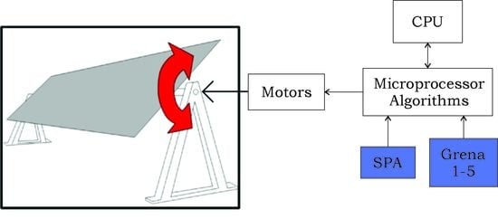
Solar trackers vary in degree of freedom and tracking technology. As for tracking technology, they may have microprocessors and optical sensors [8], algorithms based on date and time [9], or a combination of both [10]. The tracking strategy based on date and time has a computer or processor that calculates the Sun position employing algorithms that use date, time, and geographic information from the installation as input data [11]. This technology is the most used in photovoltaic plants due to its ease of implementation and lower cost when compared to other technologies.

The irradiance at a given location and time depends on the relative position between the Sun and the Earth. For this reason, the solar position calculation is important in photovoltaic systems [12]. Disturbances caused by precession and nutation of the Earth’s axis, the Moon, and other planets, among other disturbances affects the apparent movement of the Sun. These disturbances need to be considered for an accurate calculation [13].

There are several Sun position calculation algorithms available on the literature [12,13,14,15,16,17,18,19,20,21,22]. These algorithms have different processing complexity, precision, and validity time. The maximum errors of these algorithms vary from 0.0003° to units of degrees. Some of them have expired or do not work correctly for the southern hemisphere.

These algorithms have several applications in solar energy. They can be applied in solar trackers, Concentrated Solar Power (CSP), irradiance measurement instruments, and in photovoltaic system design software. The application defines the precision demanded by the algorithm. CSPs require algorithms with an accuracy of about 0.01°. Measuring instruments, e.g., pyrheliometers to measure the direct normal irradiance, demand more accurate algorithms. Photovoltaic systems admit errors up to a few degrees without expressive losses in energy generation [13].

In the literature, the publications only presented statistical analysis of the errors of the Solar Position Algorithms. Grena [13] developed a statistical analysis comparing the results of his algorithms with those of Blanco-Muriel [22], Michalsky [20], and Grena [14]. The parameters analyzed were the errors of the angles of right ascension, declination, hour angle, zenith, azimuth, and solar vector by calculating the standard deviation and maximum error. The Solar Position Algorithm (SPA) [15] was used to obtain reference values. A total of 20 million samples of dates between 2010 and 2110, random times, and localities were collected. Blanc and Wald [12] presented a statistical analysis comparing their results with the results of ESRA [23], Michalsky [20], and Grena [14]. 20,000 random samples were collected between 1980 and 2030, at daytime, at 45° N and longitude 0°. The parameters analyzed were the zenith, azimuth, and solar vector errors by calculating mean bias error, root mean square error, and maximum of absolute error.

An important parameter to be analyzed is the energy generation. For the solar plant designer, in the end, the amount of energy generated is more important than the accuracy of the angle. However, there is no published work analyzing the annual energy generation by different solar position calculation algorithms application. For this important analysis, this paper presents simulations of energy generation estimation with the application of SPA and Grena 1–5 algorithms in horizontal single-axis solar trackers.

This paper presents, in Section 2, the solar position calculation algorithms. In Section 3, the materials and methods are described. The results are discussed in Section 4, furthermore, Section 5 presents the conclusions.

2. Solar Position Calculation Algorithms

The solar position calculation algorithms available in the literature vary in accuracy, complexity, validity range, input data, and output data. Some of them calculate only global coordinates or time equation, while others also calculate topocentric coordinates of the Sun, solar incidence angle, and sunrise and sunset time. The first publications presented these algorithms like a simple step to calculate the incident solar irradiance. Due to the importance of this step in the precision of the irradiance estimation, the scientific community began too deepen and publish papers focused only on calculating the Sun position.

Cooper [16] mentioned the solar position calculation just as a simple step to calculate the fraction of incident solar irradiance that is effectively used in CSPs, without pointing out precision or validity range.

Swift [17] presented the solar position calculation as a step in the potential solar irradiance computation on slopes through measurements of irradiance on close horizontal surfaces. The solar position is calculated from the declination estimation as a function of the Julian Day. At the time, it was considered a simplification, since it avoided the use of tables for the declination estimation.

Pitman and Vant-Hull [18] presented equations for calculating the ecliptic coordinates of the Sun, solar declination, and time equation, based on The Astronomical Ephemeris and The American Ephemeris and Nautical Almanac [24]. They developed an algorithm called SUNLOC, which calculates the Sun position in horizontal coordinates with a maximum error of 41 s of arc without considering the effects of atmospheric refraction.

Walraven [21] developed an algorithm that also used the equations of The Astronomical Ephemeris and The American Ephemeris and Nautical Almanac [24] in a simplified way, claiming accuracy of 0.01°. The algorithm calculates solar declination, right ascension, azimuth, and elevation. For its simplification, it was necessary to disregard some of the effects that influence the Sun position. Its publication was followed by an errata [25] and some technical notes and letters to the editor [26,27,28], most of them about the algorithm of the original publication and the correction of atmospheric refraction.

Lamm [19] proposed a new analytical expression for the equation of time using Fourier series with an average absolute error of 0.65 s, reaching up to 8.5 s with the reduction of the Fourier series to four terms.

Michalsky [20] implemented an algorithm adapted from The Astronomical Almanac [29]. This algorithm has an accuracy of 0.01° between the years 1950 and 2050. It calculates solar declination, right ascension, hour angle, azimuth, elevation, equation of time, angle of incidence on a horizontal surface, and atmospheric refraction corrections. Michalsky [20] claims that previous publications made only brief comments on the accuracy of their respective algorithms, as “suitable for most engineering applications”. Its primary motivation was the fact that the last publication [21] on the topic received at least 10 technical notes and letters to the editor so that a researcher would have to read 11 works to decide which of the suggestions are important and should be implemented. The other motivation was the doubt about the accuracy of the algorithm proposed by Walraven [21]. It is important to note that in its original form, this algorithm does not work correctly for the southern hemisphere.

Blanco-Muriel et al. [22] developed an algorithm valid between 1999–2015 with an accuracy of 0.5 min of arc. The algorithm was developed to be applied in CSPs that use low-cost microprocessors. Therefore, it combines precision and processing simplicity, necessary characteristics for this application.

Blanc and Wald [12] developed an algorithm, which they called SG2, valid between 1980 and 2030, which presents a maximum solar vector error of 10 s, with the proposal of being faster than other algorithms that have the same level of accuracy. This algorithm consists of an approximation of the original Solar Position Algorithm (SPA) [15] equations, with a reduction in the number of operations. The motivation for its development was the need for an algorithm with a computational speed sufficient to calculate one million positions of the Sun in less than a minute, for the implementation of a database derived from satellite irradiance, called HelioClim [30].

The National Oceanic and Atmospheric Administration (NOAA) is an agency of the United States Department of Commerce whose mission is to predict changes in climate, oceans, and coasts and share this knowledge with others, in addition to conserving and managing coastal and marine ecosystems and resources. The NOAA website provides the NOAA Solar Calculator [31], where the calculations of the Sun position are based on the equations of the Astronomical Algorithms [32].

2.1. Solar Position Algorithm (SPA)

The main motivation for the development of the SPA algorithm [15] is the fact that the scientific community has several algorithms with different validity times, causing confusion and inconsistency, requiring the development of an algorithm valid for an extended period, and which has good accuracy. As a result, the SPA was developed, valid between the years −2000 and 6000.

Reda and Andreas [15] developed the SPA resulting from an adaptation of the equations contained in the book written by Meeus [32], The Astronomical Algorithms, with some modifications to meet solar energy applications. For example, in the book, the azimuth angle is measured towards the west from the south, while at the SPA, it is towards the east from the north. In addition, in the book, longitude is considered positive in west Greenwich, while for solar energy applications, it is considered positive in East Greenwich.

The SPA [15] uses Julian Day as a time scale. The algorithm calculates zenith, azimuth, solar angle of incidence, and sunrise and sunset time. In addition, it calculates some intermediate variables, such as solar declination, right ascension, and hour angle. Both intermediate and final outputs are available on the SPA website [33]. The SPA considers the corrections of nutation, aberration, parallax, and atmospheric refraction.

According to Blanc and Wald [12], approximately 1000 additions, 1300 multiplications, and 300 inverse trigonometric functions are required to calculate the Sun position. The implementation of this algorithm in C on an 8-Central Process Unit (CPU) machine would take approximately 2 h to calculate the solar position every second in 15 min for the 9 million usable pixels of the HelioClim database [30].

To assess the accuracy of the algorithm, the results were compared to Astronomical Almanac (AA) [34] data. The values of apparent right ascension, ecliptic latitude and longitude, and apparent solar declination were compared. The samples used in this comparison were related to 00:00 h on the second day of each month in the years 1994, 1995, 1996, and 2004, as it is the only AA [34] availability. This comparison analysis resulted in a maximum difference of 0.00003° in zenith and 0.00008° in azimuth. However, note that the analysis considered only 48 samples.

2.2. Grena

The primary motivation for the development of the algorithms proposed by Grena [13], which in this work are called Grena 1–5, was the fact that most of the other existing algorithms guarantee proper functioning in a period that has already expired or is expiring. He proposed five algorithms valid between the years 2010 and 2110, which can be used in photovoltaic power plants that are yet to be built. The five algorithms vary in precision and complexity, but the input and output parameters are the same.

Grena [13] compared the output data of the five algorithms with those of Michalsky [20], Blanco-Muriel [22], and an algorithm published by Grena [14] previously. The comparison is performed through the calculation of maximum and minimum errors and standard deviation using 20 million random samples. The reference values are those obtained by SPA [15]. Computational speed and validity time are also compared. The maximum errors of solar vector presented by the five algorithms are 0.2°, 0.04°, 0.01°, 0.01°, and 0.0027°, respectively. Grena 5 has better accuracy when compared to the other four algorithms, and despite being the most sophisticated algorithm of the five proposed, when compared to SPA, it has low complexity.

Each algorithm has two versions, the short and the full. The short algorithm has as output data only right ascension, solar declination, and hour angle. While the full version has as output data, in addition to the angles calculated by the short algorithms, the zenith and azimuth angles. It is impossible to calculate atmospheric refraction in short algorithms, as this calculation requires solar elevation. Therefore, the short version can only be used when atmospheric refraction can be disregarded. Another problem related to the use of short algorithms is that they only calculate geocentric coordinates, that is, coordinates that have the Earth’s center as an observation point, and for applications in solar engineering, it is convenient to use topocentric coordinates, whose observation point is the Earth’s surface [13].

The construction of the algorithms consists of Fourier analysis and physical considerations that allow finding fundamental angular frequencies and formula coefficients, followed by a fine numerical adjustment for the validity time interval, using data from the SPA [15]. All five algorithms have the first and last steps in common, so what varies between them is the central body.

3. Materials and Methods

Given the previous discussions, it is possible to realize that despite the existence of several algorithms for calculating the solar position in the literature, and many statistical analyses considering the accuracy of the solar position calculations, there is no evaluation analyzing the energy generated when these algorithms are applied to solar trackers. However, this evaluation is relevant, since, in this type of application, the energy generated is the most important parameter. This evaluation can be accomplished through simulations of energy estimation, being necessary to use a computational tool that makes it possible to insert different algorithms for calculating the solar position.

3.1. Pvlib Tool and Simulations

This work was performed using the PVLIB tool [35], which is a library for modeling and analysis of photovoltaic systems, initially developed by the National Laboratory of Sandia, and has received contributions from members of the Photovoltaic Performance and Modeling Collaboration (PVPMC).

The PVLIB tool is available in MATLAB (produced by MathWorks, Natick, MA, USA) and Python versions, and the source code is in the GitHub repository [36], where it is possible to establish a collaborative development environment. While MATLAB continues to be a common choice in private labs, Python’s popularity has grown over the past decade, as it is an easy to read and write language, portable across platforms, free and open source, and has a large computing scientific community. In addition, it allows the use of a single language for the collection, processing, and analysis of data, which allows faster development and fewer bugs [37]. For the reasons mentioned, PVLIB-Python was used for the simulations of this work.

PVLIB has a class called SingleAxisTracker that allows to run single-axis solar tracker simulations. The main function of this class is called singleaxis and calculates the rotation angle of the single-axis solar tracker using the equations proposed by Lorenzo [38], for specific values of the zenith and azimuth angles. When simulating a fixed structure system, the inclination and azimuth angles of the photovoltaic panels are fixed and determined by the user, and when simulating a system with solar trackers, these angles vary during time, according to the apparent movement of the Sun. In this case, the function singleaxis is used to calculate these angles continuously.

The irradiance data used in the simulations were those measured by a solarimetric station installed in the same place where the system is installed.

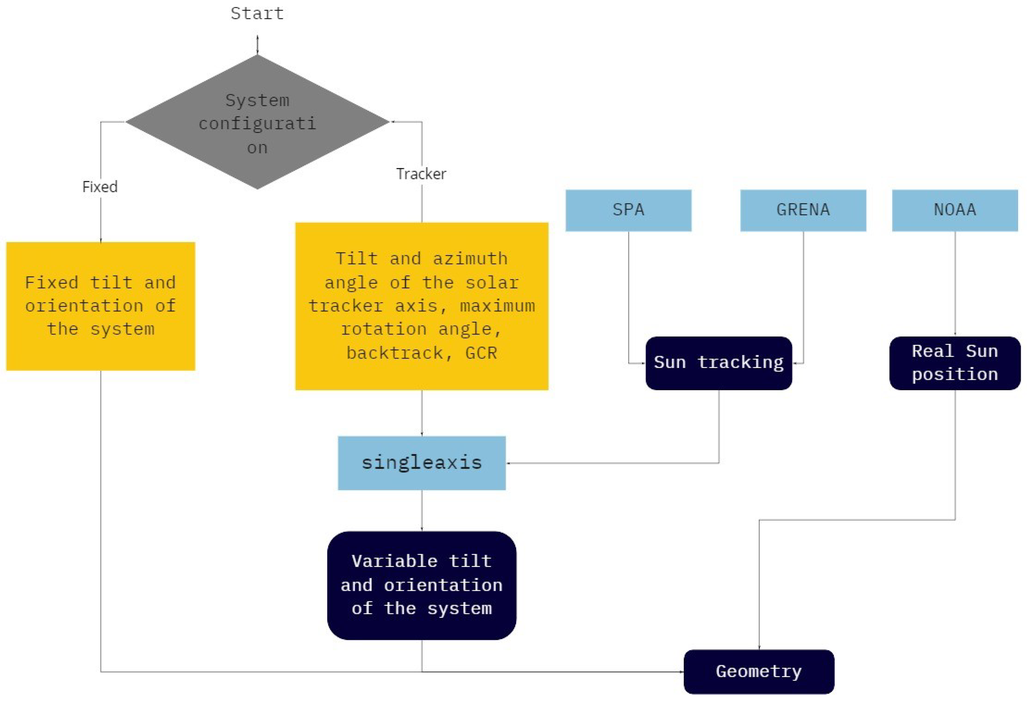
The Figure 1 and Figure 2 contain the block diagrams of the program. Among all the steps for the photovoltaic system simulation, the simulation focus of this work is that shown in Figure 2.

Figure 1 shows the simulation flow of a photovoltaic system. First, the user must enter Global Horizontal Irradiance (GHI), Diffuse Horizontal Irradiance (DHI), and Direct Normal Irradiance (DNI) data in hourly means. If all irradiance data are not available, e.g., if only GHI data are available, the decomposition process must be performed to obtain DHI, and DNI. With the GHI, DHI, and DNI data available, the transposition process is executed to obtain irradiance on tilted plane. After that, the panel model calculates the parameters of the photovoltaic panel—such as short-circuit current ($I_{sc}$), open-circuit voltage $\left(V_{oc}\right)$, current at maximum power $\left(I_{mp}\right)$, and voltage at maximum power $\left(V_{mp}\right)$—from the irradiance values on tilted plane. These values are used by the inverter model to calculate the energy generated.

Decomposition and transposition calculations require information of solar and system geometry, whose simulation processes are shown in Figure 2.

The block called geometry in Figure 2 represents the Sun’s real position and system positioning data. When it comes to simulations of systems with a single-axis solar tracker, the positioning data of the system are variable values calculated by the function singleaxis.

3.2. PV Model

This work uses the De Soto PV modeling [39]. This model uses data provided by the manufacturer, absorbed irradiance, cell temperature, and semi-empirical equations to generate the panel’s I-V curve. The equivalent circuit in Figure 3 represents the non-linear behavior of the PV module in this five-parameters model.

This modeling works to all PV module technologies and its two main Equations (1) and (2) are known from other models in literature [40]. The five parameters are a, $I_o$, $I_L$, $R_S$, and $R_{SH}$.

$$I=I_L+I_o\left[e^{\frac{V+I{R}_S}{a}}-1\right]-\frac{V+I{R}_S}{R_{SH}}$$

(1)

$$a=\frac{N_S{n}_{I}k{T}_c}{q}$$

(2)

$I_L$ corresponds to the light current (A), $I_o$ to the diode reverse saturation current (A), a to the ideality factor parameter, $R_S$ to the series resistance (Ω), and $R_{SH}$ to the shunt resistance (Ω).

The difference of De Soto model [39] is the extraction parameter method and how the parameters vary with irradiance and temperature. It is important a precise model that includes parameter variation with irradiance level due to the tracker system increases absorbed irradiance by PV modules. Particularly the parameters $I_L$ and $R_{SH}$ present influence from irradiance variation.

It is worth to note in Equation (3) the direct proportionality of $I_L$ with irradiance (S), this explains how the short-circuit current decreases or increases in the same proportion of irradiance level.

$$I_L=\frac{S}{S_{ref}}\frac{M}{M_{ref}}\left[I_{L,ref}+{\alpha }_{Isc}(T_c-T_{c,ref})\right]$$

(3)

where $S_{ref}$ corresponds to the total reference irradiance (1000 $\mathrm{W}/{\mathrm{m}}^2$), S is the total absorbed irradiance, $M/M_{ref}$ is the air mass modifier, $I_{L,ref}$ is the light current in STC, ${\alpha }_{Isc}$ is the temperature coefficient for short circuit current, $T_c$ is the cell temperature, and $T_{c,ref}$ is the cell temperature in STC (25 ${}^{\circ }$C).

In Equation (4), the relation between $R_{SH}$ and S is inversely proportional. Hence, with a irradiance increase, the shunt resistance value decreases. Then, looking back to Equation (1), it is possible to observe that a irradiance increase induces a growth in the third term ($\frac{V+I{R}_S}{R_{SH}}$), increasing internal losses in the PV module.

$$\frac{R_{SH}}{R_{SH,ref}}=\frac{S_{ref}}{S}$$

(4)

where $R_{SH,ref}$ is the shunt resistance in STC.

Then, the PV model used in this work [39] is able to represent both the current variation and the internal loss variation according to the irradiance behavior.

3.3. Methodology

Simulations of a 3.72 kWp photovoltaic system with horizontal single-axis tracker were performed to evaluate the electric energy generation of solar trackers using different algorithms for calculating the solar position. The photovoltaic system is composed of two horizontal single-axis solar trackers, each containing 6 panels of 310 Wp. The system is showed in Figure 4 and the specifications of the panels and inverters used in the simulations are shown in

Table 1. Specifications of the equipment used in simulations.

Equipment	Brand	Model	Power	Amount
Photovoltaic module	Talesun Solar®	TP762M-310	310 Wp	6
Inverter	Fronius International®	IG Plus 55 V-1	5 kW	1

.

A system of the same configuration is installed in Araçariguama, Sao Paulo, Brazil (23.444809° S; 47.108659° W), and generated 6.34 MWh of electricity in 2018. This system uses a simplified version of the SPA [15], where some coefficients are disregarded. The energy data generated by this system was used to verify that the results of the simulations are reliable.

It is important to emphasize that solar trackers aim to decrease the angle of incidence. With two-axis solar trackers, this angle of incidence can be approximately zero. In single-axis solar trackers, it is impossible to guarantee the condition of incidence angle close to zero for most of the day, as this device only has one degree of freedom. However, it is possible to guarantee the improvement of generation efficiency with the reduction of the incidence angle. The irradiance absorbed by the panel is indirectly proportional to the incidence angle, so the less the incidence angle, the higher the absorbed irradiance.

The algorithms analyzed in this study were SPA [15] and 5 algorithms developed by Grena [13], which in the present work are called Grena 1, Grena 2, Grena 3, Grena 4, and Grena 5.

These algorithms were chosen because they are the only ones that remain valid for an acceptable time to be implemented in the construction of a photovoltaic power plant and work appropriately for both hemispheres. In addition to these, three more algorithms are still valid: Michalsky [19], valid between the years 1950 and 2050, but it does not work correctly for the southern hemisphere; the algorithm proposed by the same author of Grena 1–5 [14] and the SG2 algorithm [12], however, they expire in the year 2023 and 2030, respectively, making its application in future projects unfeasible.

In Figure 2, the function singleaxis needs data from the solar position to track the Sun and return variable values of inclination and orientation of the photovoltaic panels. The data of the solar position can be calculated by the NOAA, SPA, and Grena algorithms. Seven scenarios were analyzed, each considering different algorithms when calculating the tracking of the Sun of the solar trackers. The considered scenarios are shown in

Table 2. Simulation scenarios.

Scenario	Algorithm Used to Calculate the Real Sun Position	Algorithm Used by Solar Trackers
1	NOAA	NOAA
2	NOAA	SPA
3	NOAA	GRENA 1
4	NOAA	GRENA 2
5	NOAA	GRENA 3
6	NOAA	GRENA 4
7	NOAA	GRENA 5

.

As there is no data for measuring the Sun position, the reference values for the zenith and azimuth angles considered in this work were computed on the NOAA website, using the NOAA Solar Calculator [31]. That is, these data represent the real Sun position in the simulations presented in this work.

The first scenario is, therefore, considered the ideal scenario, in which the solar tracker performs the ideal Sun tracking. In the other scenarios, the algorithms SPA and Grena 1–5 are used in Sun tracking by the solar tracker. From this analysis, it is possible to identify which algorithm brings energy generation results that are closest to the results obtained in the ideal scenario.

The tilt angle of the solar axis tracker considered in the simulations was equal to 0° since it is a horizontal single-axis solar tracker. The azimuth angle of the solar tracker axis is 0° because the system on which the simulations are based is installed with azimuth 0°. Backtrack was not used, and the GCR was equal to 0.5.

In addition, all simulations were carried out considering the different transposition methods: Isotropic [41], Reindl [42,43], Klucher [44], Hay [45], and Perez [46,47,48].

The ohmic losses ($P_{losses}$) of the cables were calculated, taking into account the maximum power current ($I_{mp}$) changes, according to Equation (5), where R is the cable resistance, which was considered to be 3.39 ohms/km. The average distance from the panels to the inverter was 10 m.

$$P_{losses}=R\times I_{mp}^2$$

(5)

After conducting the system simulations in Araçariguama, Brazil and verifying the reliability of the simulations, simulations of a system with the same configuration were performed for the cities of Cape Town, South Africa (33.932304° S; 18.429449° E), and Kiruna, Sweden (67.855812° N; 20.225013° E), to evaluate the energy generation estimation with different algorithms applied to single-axis solar trackers in different locations. In these cases, due to the absence of measured solarimetric data, data from Meteonorm 7.2 were used.

4. Results

Table 3. Result of energy generation estimation using different algorithms for Sun tracking in Araçariguama, Brazil.

Scenario	Algorithm Used by Sinle-Axis Solar Trackers	Energy Generation Estimation (MWh)
		Isotropic	Reindl	Klucher	Hay	Perez
1	NOAA	6.012594	6.338760	6.325719	6.305979	6.543707
2	SPA	6.012589	6.338758	6.325716	6.305976	6.543706
3	GRENA 1	6.012265	6.338174	6.325364	6.305391	6.543678
4	GRENA 2	6.012222	6.338105	6.325319	6.305324	6.543659
5	GRENA 3	6.012219	6.338104	6.325317	6.305321	6.543657
6	GRENA 4	6.012219	6.338103	6.325317	6.305321	6.543657
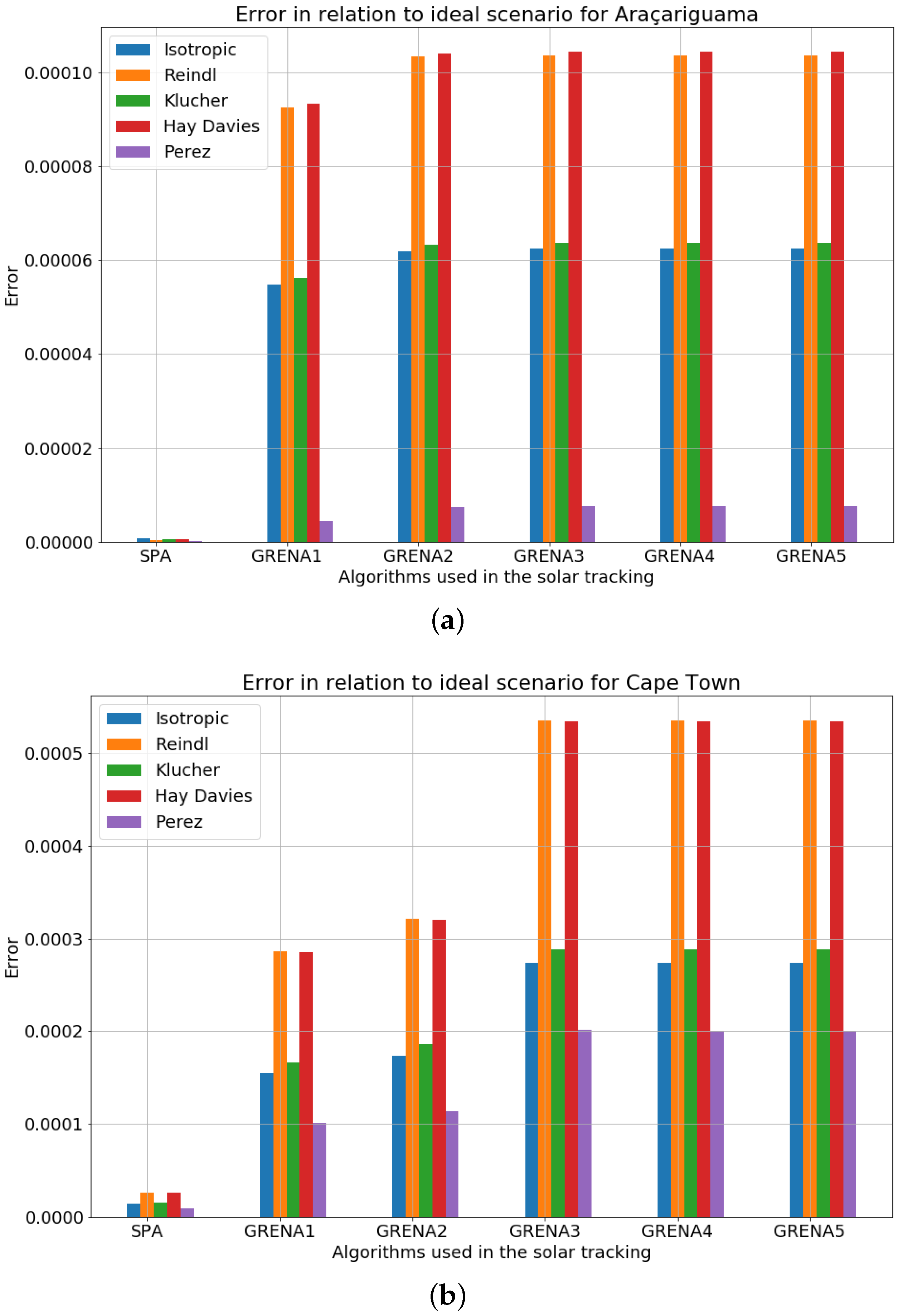
7	GRENA 5	6.012218	6.338103	6.325316	6.305321	6.543657

contains the results of energy generation estimation using different solar position calculation algorithms applied to horizontal single-axis solar trackers in the Araçariguama location. The errors in relation to the ideal scenarios are shown in Figure 5a.

The algorithm that reproduced the energy generation estimation results closest to the ideal scenario was the SPA, with errors of 0.00008%, 0.00003%, 0.00005%, 0.00005%, and 0.00002% for the Isotropic, Reindl, Klucher, Hay and Perez model of transposition, respectively. Followed by the Grena 1 and 2 algorithms, with errors of 0.00044% and 0.00073%, respectively, for the Perez model of transposition.

It is relevant to note that the results show an insignificant difference between them, with maximum errors in the order of 0.010% in relation to the ideal scenario. Therefore, in this location, any of the algorithms studied in this work can be used without incurring significant losses of energy generated.

It is worth to notice that the results of energy generation estimation for all algorithms are close to the real measurements of energy generation of the installed system, 6.34 MWh. The errors are approximately 5% for the Isotropic model of transposition and approximately 1% for the Reindl model of transposition, which rectifies the reliability of the simulations.

As the results of energy generation estimation were very close, it is important to perform the same simulation in other locations, to verify whether it is possible to extrapolate the conclusion concerning the indifference about the algorithm to be used in Sun tracking. For this purpose, Cape Town in South Africa and Kiruna in Sweden were chosen, and the results of energy generation estimation using different algorithms in Sun tracking are shown in

Table 4. Result of energy generation estimation using different algorithms for Sun tracking in Cape Town, South Africa.

Scenario	Algorithm Used by Sinle-Axis Solar Trackers	Energy Generation Estimation (MWh)
		Isotropic	Reindl	Klucher	Hay	Perez
1	NOAA	8.069870	8.564122	8.405154	8.538255	8.549887
2	SPA	8.069754	8.563903	8.405026	8.538035	8.549813
3	GRENA 1	8.068618	8.561675	8.403759	8.535820	8.549020
4	GRENA 2	8.068471	8.561373	8.403594	8.535521	8.548916
5	GRENA 3	8.067663	8.559537	8.402732	8.533688	8.548169
6	GRENA 4	8.067663	8.559538	8.402732	8.533688	8.548170
7	GRENA 5	8.067663	8.559538	8.402733	8.533689	8.548171

and

Table 5. Result of energy generation estimation using different algorithms for Sun tracking in Kiruna, Sweden.

Scenario	Algorithm Used by Sinle-Axis Solar Trackers	Energy Generation Estimation (MWh)
		Isotropic	Reindl	Klucher	Hay	Perez
1	NOAA	3.393033	3.637877	3.548495	3.623429	3.841570
2	SPA	3.393026	3.637872	3.548489	3.623424	3.841570
3	GRENA 1	3.392167	3.636253	3.547614	3.621843	3.840457
4	GRENA 2	3.392249	3.636323	3.547680	3.621917	3.840865
5	GRENA 3	3.392271	3.636339	3.547702	3.621935	3.840877
6	GRENA 4	3.392268	3.636337	3.547698	3.621932	3.840876
7	GRENA 5	3.392269	3.636339	3.547700	3.621933	3.840877

, respectively.

Regarding the energy generation estimation results for Cape Town, Africa, it can be seen that the algorithm that obtained the least error in relation the ideal scenario was the SPA, with an error of 0.00087%, followed by the Grena algorithms 1 and 2, with errors of 0.01014% and 0.01136%, respectively, for the Perez’s transposition model. Likewise, it can be noticed by the Figure 5b that the results of the other algorithms were very close, with maximum errors of the order of 0.0005% for all transposition models. Leading to the conclusion that, in this location, any algorithm can be used without considerable losses in energy generation.

In the simulations performed for Kiruna, Sweden, the SPA obtained the lowest error compared to scenario 1, approximately 0.0%, followed by the Grena 3, 4, and 5 algorithms, with an error of 0.0181% for the Perez’s transposition model. This behavior is repeated for the other transposition models.

In all the sites analyzed, the SPA showed a smaller error in relation to the ideal scenario. However, as the difference between the results of energy generation simulation are small, it can be overlooked. Therefore, the user can apply any of theses algorithms in horizontal single-axis solar trackers without significant losses in energy generation. For designers interested in less computational effort, Grena 1 and Grena 2 are highlighted for less complex implementation and faster processing.

5. Conclusions

Simulations of energy estimation were performed using different algorithms for calculating the Sun position applied to horizontal single-axis solar trackers. The simulated system has the same characteristics of a system installed in Araçariguama, Sao Paulo, Brazil. From the results, it was possible to observe that the energy generation estimation through simulations were close to the energy measurement results of the installed system, ensuring the reliability of the simulations.

The algorithm that obtained the results of energy generation estimation closest to the ideal scenario was the SPA, with errors of approximately 0.00002%, 0.00087%, and 0.0% for the locality of Araçariguama—Brazil, Cape Town—South Africa, and Kiruna—Sweden, respectively. However, the results of the Grena 1–5 algorithms showed an insignificant difference for all the performed simulations. Such results allow concluding that, regarding horizontal single-axis solar tracking, any of the 6 algorithms analyzed in this work can be used without incurring relevant errors in the estimation of the energy that can be generated.

Therefore, given the statements of the literature about the complexity and the processing speed of each algorithm, for designers who are interested in reducing computational cost, it would be recommended to use the Grena 1 and Grena 2 algorithms, since they are less complex and faster.