Article

Optimal Chiller Loading for Energy Conservation Using an Improved Fruit Fly Optimization Algorithm

1
College of Computer Science, Liaocheng University, Liaocheng 252059, China
2
School of Information Science and Engineering, Shandong Normal University, Jinan 250014, China
*
Authors to whom correspondence should be addressed.
Energies 2020, 13(15), 3760; https://doi.org/10.3390/en13153760
Submission received: 6 June 2020 / Revised: 15 July 2020 / Accepted: 18 July 2020 / Published: 22 July 2020
(This article belongs to the Section G: Energy and Buildings)

Abstract

:
In the multi-chiller of the air conditioning system, the optimal chiller loading (OCL) is an important research topic. This research is to find the appropriate partial load ratio (PLR) for each chiller in order to minimize the total energy consumption of the multi-chiller under the system cooling load (CL) requirements. However, this optimization problem has not been well studied. In this paper, in order to solve the OCL problem, we propose an improved fruit fly optimization algorithm (IFOA). A linear generation mechanism is developed to uniformly generate candidate solutions, and a new dynamic search radius method is employed to balance the local and global search ability of IFOA. To empirically evaluate the performance of the proposed IFOA, a number of comparative experiments are conducted on three well-known cases. The experimental results show that IFOA found 14 optimal values (the optimal values among all algorithms) under a total of 17 CLs in three cases, and the ratio of the optimal values found was 82.4%, which was the highest among all algorithms. In addition, the mean value of all objective functions of IFOA is smaller and the standard deviation is equal to or close to 0, which proves that the algorithm has high stability. It can be concluded that IFOA is an ideal method to solve the OCL problem.

1. Introduction

To maintain comfort level of an indoor life during hot and humid weather, many people rely on air-conditioning systems. Thus, air-conditioning systems are used in large quantities, and their energy consumption for the supply of CL accounts for more than 30% of the total power generation [1]. In air-conditioning systems, the multi-chiller system is the main energy-consumption equipment. If the chillers are improperly managed, the energy consumption of the chiller will be increased significantly. Because the multi-chiller system is composed of chillers of different design capacities and performance feature, the optimal load distribution of each chiller can obtain minimum energy consumption when meeting CL demand [2]. Therefore, for the part load ratios of all chillers, it is a valuable research topic to find their optimal combination by using optimization methods.
Recently, significant efforts have been made in applying evolutionary optimization algorithms to solve the OCL problem, such as the Lagrangian method (LM) [3], branch and bound (B&B) [4], genetic algorithm (GA) [5,6], simulated annealing (SA) [7,8], particle swarm optimization (PSO) [1,9], evolution strategy (ES) [10], gradient method (GM) [11], generalized reduced gradient (GRG) [12], differential evolution (DE) [13,14], improved firefly algorithm (IFA) [15], differential search (DS) [16], neural networks model with particle swarm optimization (NNPSO) [17], cuckoo search algorithm using a differential operator (DCSA) [18], general algebraic modeling system (GAMS) [19,20], teaching–learning-based optimization (TLBO) [21], exchange market algorithm (EMA) [22], improved grasshopper optimization algorithm (CGOA) [23], improved invasive weed optimization (EIWO) [24], improved artificial fish swarm algorithm (VAFSA) [25], information gap decision theory (IGDT) [26], Q-learning method [27], and distributed chaotic estimation of distribution algorithm (DCEDA) [28]. Among them, DCEDA has achieved the best results to date.
The fruit fly optimization algorithm (FOA, also known as canonical FOA) is a new swarm intelligence optimization algorithm, proposed by Pan [29] in 2011. FOA was inspired by the foraging behavior of fruit fly swarms, and the optimization is performed based on competition and cooperation among fruit flies. The FOA has many advantages, i.e., a simple principle and few adjustment parameters, and can be realized easily. At the same time, it has a very high convergence speed. In view of this, FOA has been applied successfully in many fields [30,31,32,33,34,35,36,37,38,39,40,41]. The existing literature has demonstrated that FOA is competitive compared with GA, PSO, SA, and other heuristic algorithms. However, there is no literature using FOA in solving OCL problems currently. Hence, in our work, to solve the OCL problem, an improved fruit fly optimization algorithm is proposed.
The rest of this paper is organized as follows. Section 1 gives a brief introduction. Section 2 provides a description of the multi-chiller system. Section 3 introduces the canonical FOA and analyzes its disadvantages. The improved FOA, which uses the dynamic search radius method, is introduced in Section 4. Section 5 presents the implementation of IFOA on solving OCL problem. In Section 6, empirical comparative results on three well-known cases are presented and discussed. Finally, the conclusions are given in Section 7 and the future work is prospected.

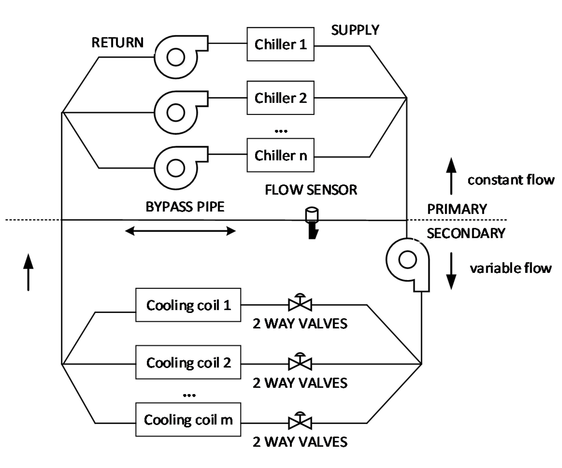
2. Problem Description

Due to the large demand for cooling in massive buildings, the multi-chiller system is generally used. Figure 1 depicts the structure of a typical multi-chiller decoupled system. It consists of a primary side (chiller side) and a secondary side (load side) [2]. On the primary side, multiple chillers are connected to the distributed system in series or parallel. The system allocates different loads to each chiller by controlling the supply and return water flow because each chiller has different capacities. On the secondary side, the cold water flowing into the cooling coil can be adjusted by a two-way valve according to load changes.
The multi-chiller system is designed to meet peak loads, but most of the time, the chiller operates at partial load ratio. PLRi can be calculated using Equation (1) [2]. Here, CLi represents the ith chiller CL, and RTi represents its design capacity (RT). Equation (1) is the expression of the meaning of PLR, but we do not use Equation (1) to calculate the value of PLR. The value of PLR is obtained through the IFOA iterative optimization proposed in the paper. Obviously, the value range of the PLR should be in the range [0,1], but when PLR is small, the chiller is prone to surge, thus, the manufacturer recommends that the PLR of each chiller should be greater than or equal to 30%, as shown in Equation (2). Here ONi is the state of the ith chiller. When ONi = 1, it is on; when ONi = 0, it is off. In a multi-chiller system, in order to minimize energy consumption, one or several chillers are allowed to not start up, that is, their PLR is 0. Equation (2) is the constraint condition that the OCL problem must satisfy:
P L R i = C L i R T i
P L R i = { r a n d ( 0.3 , 1 )   i f   O N i = 1   0   i f   O N i = 0  
For a given wet-bulb temperature, the power consumption (P) of a centrifugal chiller is a convex function of its PLR [6]. Pi is expressed as a polynomial of PLRi, as shown in Equation (3):
P i = { c 1 i + c 2 i · P L R i + c 3 i · P L R i 2   i f   O N i = 1   ( u s e d   b y   c a s e   1 ) c 1 i + c 2 i · P L R i + c 3 i · P L R i 2 + c 4 i · P L R i 3   i f   O N i = 1   ( u e s e d   b y   c a s e   2   a n d   c a s e   3 ) 0   i f   O N i = 0
Here, c1i, c2i, c3i, c4i are constants, representing the coefficients of the ith chiller KW-PLR curve, respectively.
Cases 1, 2, and 3 correspond to the case study with six, four, and three chillers in Section 6, respectively.
Finding the minimum value of the total energy consumption is the objective function of the OCL problem in the multi-chiller system, as given in Equation (4):
J = min ( i = 1 n P i )
where Pi represents the ith chiller power consumption and n is the total number of chillers.
The sum of the CLs generated by all the chillers in the multi-chiller system should not be less than the system CL demand. This constraint must be satisfied, and can be denoted using Equation (5):
i = 1 n P L R i · R T i C L  
Under the condition of satisfying CL requirements, if the total energy consumption of all chillers is minimized, then the performance of multi-chiller system is the best [15]. The functional objective of the OCL problem is to minimize the total energy consumption of multi-chiller, that is, the value of J obtained in Equation (4) is the minimum. The constraints of the OCL problem are Equation (2) and (5), that is, the PLR of each chiller must be greater than or equal to 0.3, and the CL generated by multi-chiller must satisfy the system CL demand. The solution to the OCL problem is the appropriate PLR value for each chiller in a multi-chiller.

3. Canonical FOA and Analysis

3.1. Canonical FOA Overview

Canonical FOA is the basic version of FOA proposed by Pan in 2011. In order to show the difference from the various FOA versions improved later, we generally call it “canonical FOA”. The canonical FOA adopts a global random search strategy based on swarm. In each generation, there are two phases of osphresis and vision foraging. In the osphresis foraging phase, each individual in the fruit fly swarm searches randomly around swarm, and then finds the maximum smell concentration of the individual after evaluating the new location. In the vision foraging phase, all individuals fly to the location where smell concentration is maximum. The canonical FOA has four steps.
Step 1. Initialization.
Set parameters such as the population size (PS), the maximum number of iterations (Itermax), the random fly direction and distance zone of fruit fly (FR), and the fruit fly swarm location range (LR). The location of fruit fly individual in the swarm is given by its corresponding two-dimensional coordinates (X, Y), whose initial location is defined by Equation (6):
{ X _ a x i s = r a n d ( L R ) Y _ a x i s = r a n d ( L R )
Here the function of rand(LR) is to get a number arbitrarily within the range of the positions of the fruit fly swarm.
Step 2. Osphresis foraging phase.
Step 2.1. Using the osphresis organ, fruit fly individuals search randomly around the swarm. Each individual is given a flight direction and distance randomly. The new location of the individual is computed by Equation (7):
{ X i = X _ a x i s + r a n d ( F R ) Y i = Y _ a x i s + r a n d ( F R )
Here the function of rand(FR) is to get a number arbitrarily within the fly range of the fruit fly.
Step 2.2. The distance (DISTi) between the individual and the origin is calculated using Equation (8) due to the exact location of the food being unknown. Then, the smell concentration judgment value (Si) of a fruit fly individual is computed by Equation (9), which is the reciprocal of the distance:
D I S T i = X i 2 + Y i 2
S i = 1 / D I S T i
Step 2.3. The smell concentration (Smelli) of each fruit fly individual in the swarm is calculated by Equation (10), that is, Si is substituted into the fitness function (or smell concentration judgment function):
S m e l l i = f i t n e s s ( S i )
Step 2.4. Find the fruit fly with the best smell concentration in the swarm and record its smell concentration and corresponding location, as shown in Equation (11):
[ b e s t S m e l l , b e s t I n d e x ] = m i n ( S m e l l )
Step 3. Vision foraging phase.
The best smell concentration value and corresponding fruit fly location are maintained by Equations (12) and (13), respectively, and other fruit flies will use vision to fly toward that location:
S m e l l b e s t = b e s t S m e l l
{ X _ a x i s = X ( b e s t I n d e x ) Y _ a x i s = Y ( b e s t I n d e x )
Step 4. Repeat steps 2 and 3 until Iter reaches Itermax.

3.2. Disadvantages of Canonical FOA

By analyzing the canonical FOA algorithm, two disadvantages of FOA can be summarized as follows.
(1)
Nonuniform generation of candidate solutions
Shan et al. [42] first substituted Equation (7) into Equation (8). In Equation (8), X _ a x i s and Y _ a x i s are constants, and rand(FR) is a variable. Then they used the counter-proof method to prove that for the given fruit fly position coordinates X and Y, the taste concentration judgment value Si does not follow a uniform distribution. Usually, Si is the solution to the optimization problem. Obviously, the candidate solutions cannot be generated uniformly, that is, FOA loses the ability to search uniformly in the solution space.
(2)
Poor search ability
The search radius of the fruit fly is its range of flight (FR). When the FR is large, the search range of fruit fly is large, and the global search ability of FOA is strong, while when the FR is small, the search range of fruit fly is small, and the local search ability of FOA is strong. In the canonical FOA, FR is a fixed value, which cannot better balance the global search ability and local search ability of the algorithm.

4. Improved FOA Algorithm Based on Dynamic Search Radius

To overcome the first disadvantage summarized above, we should first find the cause of the disadvantage. An analysis of Equations (6)–(9) found that the location of an individual can be represented by two-dimensional coordinates, and the candidate solution is the reciprocal of the distance between individual location and the origin. The candidate solutions generated by FOA are nonlinear, thus, they fail to follow the uniform distribution.
Inspired by the reference literature [42], for FOA, we can change the non-linear of the candidate solution generation mechanism into a linear one, that is, the location of the individual is represented by one-dimensional coordinates, and we no longer calculate the reciprocal of the distance between individuals and the origin. Thus, the original equations have been modified. That is, Equations (6), (7), (9), and (13) are changed into Equations (14)–(17), respectively, and Equation (8) is deleted.
The advantage of using this linear generation mechanism is that candidate solutions can be generated uniformly in the solution space, so that the swarm has the ability to search the global optimal solution:
X _ a x i s = r a n d ( L R )
X i = X _ a x i s + r a n d ( F R )
X _ a x i s = X ( b e s t I n d e x )
S i = X i
For the second disadvantage mentioned above, this paper proposes a new dynamic search radius method that changes the search radius by the iteration number, as shown in Figure 2. Therefore, the search radius can cover the entire solution space in early iterations, which gives the algorithm a good global search capability. In later iterations, the search radius becomes very small when the swarm location is close to the best solution, which guarantees that the algorithm will have a good local search capability. The search radius r can be obtained by Equation (18):
r = ( r m a x r m i n ) · e x p ( 10 I t e r 2 I t e r m a x 2 ) + r m i n
where rmin is the minimum search radius, rmax is the maximum search radius, Itermax is the maximum number of iterations, and Iter is the number of iterations.
A good initial swarm location can make the algorithm converge faster. Therefore, in the improved FOA, a population is generated randomly, and then, the location of the optimal individual is selected as the initial swarm location instead of the location generated according to Equation (14). The improved FOA algorithm based on the dynamic search radius is called IFOA. Algorithm 1 shows the main structure of IFOA.
Algorithm 1. Improved fruit fly optimization algorithm (IFOA) algorithm
Parameters: PS, Itermax, rmax, rmin
Output: Solution X*
//Initialization
Set PS, Itermax, rmax, rmin
Fori = 1, 2, …, PS
        X i = r a n d ( L R ) //Generate the locations of PS individuals
        S i = X i
        S m e l l i = f i t n e s s ( S i )
        [ b e s t S m e l l , b e s t I n d e x ] = min ( S m e l l )
Endfor
X _ a x i s = X ( b e s t I n d e x ) //Set swarm location
Iter = 0, X* = X_axis
Repeat
          r = ( r m a x r m i n ) · e x p ( 10 I t e r 2 I t e r m a x 2 ) + r m i n
    //Osphresis foraging phase
    For i = 1, 2, …, PS
                X i = X _ a x i s + r · r a n d ( )
                S i = X i
                S m e l l i = f i t n e s s ( S i )
                [ b e s t S m e l l , b e s t I n d e x ] = min ( S m e l l )
    Endfor
    //Vision foraging phase
    if Smellbest > bestSmell then
  Smellbest = bestSmell
                X _ a x i s = X ( b e s t I n d e x )
    Iter = Iter + 1
UntilIter == Itermax

5. Implementation of IFOA on OCL Problem

When using IFOA to solve the OCL problem, each individual in the fruit fly swarm corresponds to a solution in the problem. Taking a multi-chiller composed of three chillers as an example, the PLR value of each chiller is represented by a decimal code value, and the encoded values of the three chillers constitute a fruit fly individual, as shown in Figure 3, where each PLR value must satisfy the constraints given by Equation (2).
Step 1. Initialization.
First determine the center of a good fruit fly swarm. Randomly generate an initial swarm of fruit fly composed of PS fruit fly individuals, calculate the energy consumption of each chiller according to Equation (3), and then obtain the total energy consumption of multi-chiller system by Equation (4). The energy consumption of all PS multi-chiller systems is calculated accordingly. After substituting the PLR values of the three chillers into Equation (5), the total cooling output is obtained and compared with the CL demand of the system. The value of the fitness function of the multi-chiller that satisfy the constraints is equal to its energy consumption value, and the value of the fitness function of the multi-chiller that does not satisfy the constraints is given a larger penalty value. Find the fruit fly with the smallest fitness function value in the swarm, and take the position of this fruit fly as the center position X_axis of the swarm.
Taking Figure 3 as an example, the data of the three chillers are in Ref. [6], and their rated cooling capacity is 800RT. The calculation process is as follows:
  • P1 = 100.95 + 818.61 × 0.6588 − 973.43 × (0.6588)2 + 788.55 × (0.6588)3 = 443.235317 KW,
  • P2 = 481.473064 KW, P3 = 478.487741 KW,
  • J = P1 + P2 + P3 = 1403.196121 KW,
  • 0.6588 × 800 + 0.8589 × 800 + 0.8823 × 800 = 1920RT, 1920RT = CL.
Step 2. Osphresis foraging phase.
Find the search radius r according to Equation (18), then use the equation X i = X _ a x i s + r · r a n d ( ) to find the position of the fruit fly, and a swarm of PS fruit fly individuals is generated according to this method. Next, calculate the total energy consumption, total cooling output, and fitness function values of the multi-chiller separately. The calculation method is the same as Step 1.
Step 3. Vision foraging phase.
Find the fruit fly with the smallest fitness function value in the swarm, and take the position of this fruit fly as the center position X_axis of the swarm.
Step 4. Repeat steps 2 and 3 until Iter reaches Itermax.
After the iteration is terminated, the coding of the fruit fly individual with the smallest fitness function value is the solution to the OCL problem.

6. Simulation Results

6.1. Cases Used in Experiments

In the experiments, three well-known cases are selected to verify the performance of IFOA in solving the OCL problem.

6.1.1. Case with Six Chillers

Case 1 is based on the multi-chiller system of a semiconductor plant located in Hsinchu Science Garden (Taiwan), and was originally proposed by Ref. [6]. It consists of six chiller units. Among them, the capacity of four units is 1280RT, and the other two units are 1250RT. Table 1 lists the chiller data for the first case that can be used in Equation (3).

6.1.2. Case with Four Chillers

Case 2 is based on the multi-chiller system in a hotel located in Taipei, and was originally proposed by Ref. [3]. It consists of four chiller units, among which two units have the capacity of 450RT, and two units have the capacity of 1000RT. Table 2 lists the chiller data for the second case that can be used in Equation (3).

6.1.3. Cases with Three Chillers

The multi-chiller system in Case 3 is also a semiconductor factory located in Hsinchu Science Garden, which uses three chillers with a design capacity of 800RT [6]. Table 3 lists the chiller data for the third case that can be used in Equation (3).

6.2. Results and Analysis

The IFOA algorithm was implemented in the Visual Studio 2010 environment using C++ and run on the Intel Core i5–9300H 2.40 GHz PC. IFOA was run 30 times independently considering that unexpected situations may occur. The maximum, minimum, mean, and standard deviation were calculated from 30 optimal objective function values to comprehensively evaluate the IFOA algorithm’s ability to solve the OCL problem.
The optimal results of IFOA (the minimum of 30 optimal objective function values) are compared with those of some algorithms. We bold the optimal value of the algorithms and the reduction in energy consumption of IFOA.
IFOA has four control parameters, and their setting values are shown in Table 4.

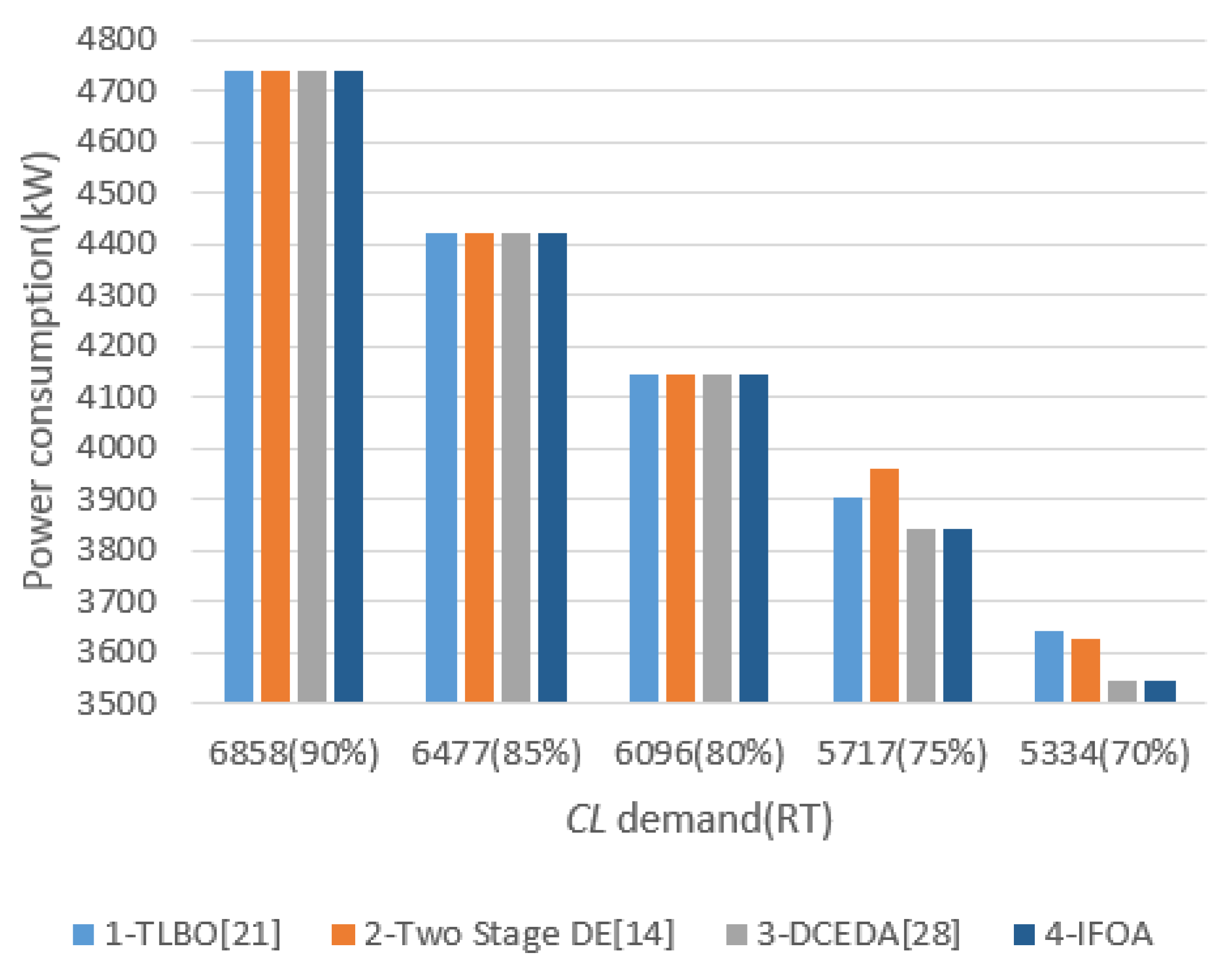
6.2.1. Comparisons of the First Case Experiment

Table 5 summarizes the comparison of the optimal values of IFOA and TLBO [21], Two Stage DE [14], and DCEDA [28]. As can be seen from the table, (1) when CL is 6858, 6477, and 6096, IFOA is equal to Two Stage DE and DCEDA; (2) when CL is 5717, 5334, IFOA saves 116.16 KW and 81.337 KW more than Two Stage DE and 0.517 KW and 0.043 KW more than DCEDA. It is particularly emphasized here that we added the strikethrough to the optimal values 3838.2079 and 3507.269 obtained by Two Stage DE, because these two values are wrong. Taking the optimal value of 3838.2079 as an example, let us restore its calculation process:
  • P1 = 399.345 − 122.12 × 0.843243 + 770.46 × (0.843243)2 = 844.210495 KW,
  • P2 = 287.116 + 80.04 × 0.783222 + 700.48 × (0.783222)2 = 779.505229 KW,
  • P3 = −120.505 + 1525.99 × 0.000000 – 502.14 × (0.000000)2 = −120.505 KW,
  • P4 = 781.488298 KW, P5 = 755.200502 KW, P6 = 798.313427 KW,
  • J = i = 1 6 P i   = 3838.212951 KW.
The PLR value here retains six digits after the decimal point, and the PLR is a double type variable in the actual program, thus, the accuracy is reduced, resulting in a slight error in the calculation result. In other words, the J value obtained in the actual program is 3838.2079. In addition, we noticed that the value of PLR3 is 0.000000, that is, the third chiller is off, and its energy consumption should be 0. But Two Stage DE substitutes 0.000000 into the equation and obtains a value of −120.505. That is, the energy consumption of the third chiller is −120.505 KW, which is obviously unreasonable, and its actual optimal value should be 3958.7129 KW (3838.2079 + 120.505 = 3958.7129); (3) when CL is 6477, IFOA is equal to TLBO; when CL is 6858 and 6096, TLBO saves 0.035 KW and 0.066 KW more than IFOA; when CL is 5717 and 5334, IFOA saves 62.147 KW and 96.073 KW more than TLBO. Figure 4 is a histogram representation of the results in Case 1.
The optimal value of IFOA is the minimum value of the objective function obtained by running it 30 times independently. To further evaluate the stability of the algorithm, Table 6 summarizes the maximum, minimum, mean, and standard deviation of the optimal objective function values got by IFOA and DCEDA after 30 independent runs. Measure the stability of the algorithm by first comparing the mean, and if the mean is equal, compare the standard deviation. It can be seen from Table 6 that under all five CLs, the mean and standard deviation of IFOA are smaller compared to DCEDA. Therefore, we can conclude that the stability of IFOA in case 1 is better than DCEDA. In addition, we also give the running time of the algorithm in Table 6, which is the average time of 30 independent runs. It can be seen from the table that CPU time of IFOA and DCEDA is about 0.7 s for all five CLs.

6.2.2. Comparisons of the Second Case Experiment

Table 7 summarizes the optimal values of IFOA and TLBO [21], Two Stage DE [14], and DCEDA [28]. As can be seen from the table, (1) when CL is 1160, IFOA saves energy by 0.02 KW more than DCEDA, otherwise the two are equal; (2) when the CL is 2320, 1740, 1450, and 1160, respectively, IFOA saves energy by 0.073 KW, 10.679 KW, 0.043 KW, and 0.004 KW compared to Two Stage DE. In other cases, the two are equal. It is particularly emphasized here that we added the strikethrough to the optimal values 942.059, 752.963, and 583.938 obtained by Two Stage DE. The reason is the same as in Case 1. Their actual optimal values should be 1009.209 KW (942.059 + 67.15 = 1009.209), 820.113 KW (752.96 + 67.15 = 820.113), and 651.074 KW (583.938 + 67.136 = 651.074); (3) when the CL is 2610, IFOA is equal to TLBO; when the CL is 1740, TLBO saves 1.35 KW more than IFOA; when the CL is 2320, 2030, 1450, and 1160, respectively, IFOA saves energy by 0.04 KW, 0.65 KW, 87.32 KW, and 205.77 KW compared to TLBO. Figure 5 is a histogram representation of the results in Case 2.
Table 8 summarizes the maximum, minimum, mean, and standard deviation of the optimal objective function values got by IFOA and DCEDA after 30 independent runs. As seen from Table 8, in all six CLs, the mean values of the optimal objective function values of IFOA are equal to the minimum values, and the standard deviations are 0; this result proves that the stability of IFOA in Case 2 outperforms that of DCEDA. In addition, the average running times of the algorithms are given in Table 8. As can be seen from the table, the CPU time of the algorithm decreases with the decrease of CL. The CPU time of IFOA and DCEDA is approximately equal.

6.2.3. Comparisons of the Third Case Experiment

Table 9 summarizes the comparison of the optimal values of IFOA and TLBO [21], Two Stage DE [14], and DCEDA [28]. It can be seen from the table, (1) IFOA is equal to Two Stage DE and DCEDA under all six CLs; (2) when CL is 2160, 1680, 1440, 1200, and 960, respectively, IFOA saves energy by 0.01 KW, 0.02 KW, 100.95 KW, 100.945 KW, and 100.951 KW compared to TLBO, otherwise the two are equal. Figure 6 is a histogram representation of the results in Case 3.
Table 10 summarizes the maximum, minimum, mean, and standard deviation of the optimal objective function values obtained by IFOA and DCEDA after 30 independent runs. As seen from Table 10, in all six CLs, the mean values of the optimal objective function values got by IFOA equal the minimum values, and the standard deviations are 0; this result proves that the stability of IFOA in Case 3 outperforms that of DCEDA. In addition, the average running times of the algorithms are given in Table 10. As can be seen from the table, the CPU time spent by IFOA and DCEDA is around 0.1 s for all six CLs.

6.2.4. Results of Comparison of Three Case Experiments

Table 11 summarizes the results of the previous three case studies. As can be seen from the table, in Cases 1, 2, and 3, the number of optimal values (the optimal values in all algorithms) found by IFOA are 3, 5, and 6, respectively, and the ratio of the optimal values found is 60%, 83.3%, and 100%, respectively. In three cases, of a total of 17 CLs, IFOA found a total of 14 optimal values; the ratio of the optimal value found is 82.4%, and the ratio of the optimal value found in all algorithms is the highest. In addition, in order to evaluate the stability of IFOA, by comparison with DCEDA, the average value of all the objective function values of IFOA is smaller, and the standard deviation is close to or equal to 0. It can be concluded from the comparison of the above two aspects that IFOA is superior to other comparison algorithms in solving OCL problems.

7. Conclusions and Future Work

OCL is a crucial optimization problem in many realistic applications. However, this problem has not been solved well. Therefore, an efficient optimization algorithm is urgently needed to solve the OCL problem. In this study, in order to solve the OCL problem, in view of the two disadvantages of FOA, we propose an improved FOA algorithm (IFOA). The main contributions of the research are summarized as follows: (1) a mechanism for generating candidate solutions is developed. This mechanism changes the generation of candidate solutions from nonlinear to linear, so that IFOA has the ability to search uniformly in the solution space; (2) a new dynamic search radius method is proposed, which makes the search radius change smoothly with the number of iterations. In the early iterations, the large search radius gave IFOA global search ability. Then, as the number of iterations increases, the search radius gradually decreases. In the later stage of the iteration, the position of the fruit fly swarm is close to the optimal solution. At this time, a small search radius can enhance the local search ability of IFOA.
In order to verify the ability of IFOA to solve OCL problems, we selected three well-known cases to our study. The experiment results show that IFOA has two advantages: (1) strong optimization ability. The probability of IFOA finding the optimal solution is 82.4%, which is the highest among all algorithms; (2) high stability. The mean value of all objective functions of IFOA is smaller and the standard deviation is equal or close to 0. From the above two aspects, we can draw a conclusion that the IFOA algorithm is a highly recommended effective algorithm for solving OCL problems, and it can also be used in other optimization fields.
There are several opportunities for future research on optimization algorithms for the OCL problem. First, the multi-chiller load balancing problem will be considered. Then, some new multi-objective evolutionary optimization algorithms [43,44,45,46,47,48,49,50] can be used to solve the above OCL problems.

Author Contributions

Conceptualization: M.-Y.Q. and J.-X.D.; methodology: M.-Y.Q. and J.-Q.L.; software: M.-Y.Q. and J.-X.D.; validation: M.-Y.Q. and J.-Q.L.; investigation: Y.-Y.H.; data curation: M.-Y.Q. and J.-X.D.; writing—original draft preparation: M.-Y.Q.; writing—review and editing: M.-Y.Q. and Y.-Y.H.; funding acquisition: J.-Q.L. and Y.-Y.H. All authors have read and agreed to the published version of the manuscript.

Funding

This research is partially supported by the National Science Foundation of China under Grant 61803192, 61773192, 61773246, and 61603169, and the State Key Laboratory of Synthetical Automation for Process Industries (PAL-N201602).

Conflicts of Interest

The authors declare no conflict of interest.

Nomenclature

PLRpartial load ratioSmellbestthe best smell concentration in vision foraging phase
CLcooling loadrthe search radius
RTdesign capacityIFOAimproved fruit fly optimization algorithm
ONthe state of the chillerGAgenetic algorithm
Ppower consumptionSAsimulated annealing
acoefficients of the chiller KW-PLR curvePSOparticle swarm optimization
bGRGgeneralized reduced gradient
cDSdifferential search
dDCSAdifferential cuckoo search algorithm
Jthe total energy consumption of multi-chiller systemLGMLagrangian method
B&Bbranch and bound
nthe total number of chillersESevolution strategy
PSpopulation sizeGMgradient method
Iterthe number of iterationsDEdifferential evolution
LRthe fruit fly swarm location rangeIFAimproved firefly algorithm
FRthe flight rangeNNPSOneural networks model with particle swarm optimization
Xhorizontal coordinateGAMSgeneral algebraic modeling system
Yvertical coordinateTLBOteaching-learning-based optimization
DISTthe distance between the individual and the originEIWOimproved invasive weed optimization
EMAexchange market algorithm
Sthe smell concentration judgment valueCGOAimproved grasshopper optimization algorithm
Smellthe smell concentrationVAFSAimproved artificial fish swarm algorithm
bestSmellthe best smell concentration in osphresis foraging phaseIGDTinformation gap decision theory
bestIndexlocation with the best smell concentrationDCEDAdistributed chaotic estimation of distribution algorithm

References

  1. Ardakani, A.J.; Ardakani, F.F.; Hosseinian, S.H. A novel approach for optimal chiller loading using particle swarm optimization. Energy Build. 2008, 40, 2177–2187. [Google Scholar] [CrossRef]
  2. Linton, R.; Frutiger, T.; Blanc, S.; Hydeman, M.; Brambley, M.; Branson, D.; O’Neill, P.; Cagwin, D.; Kammers, B.; Carpenter, P. Ashrae Handbook; American Society of Heating, Refrigerating and Air-Conditioning Engineers, Inc.: Atlanta, GA, USA, 2008. [Google Scholar]
  3. Chang, Y.C. A novel energy conservation method―optimal chiller loading. Electr. Power Syst. Res. 2004, 69, 221–226. [Google Scholar] [CrossRef]
  4. Chang, Y.C.; Lin, F.A.; Lin, C.H. Optimal chiller sequencing by branch and boun method for saving energy. Energy Convers. Manag. 2005, 46, 2158–2172. [Google Scholar] [CrossRef]
  5. Chang, Y.C. Genetic algorithm based optimal chiller loading for energy conservation. Appl. Therm. Eng. 2005, 25, 2800–2815. [Google Scholar] [CrossRef]
  6. Chang, Y.C.; Lin, J.K.; Chuang, M.H. Optimal chiller loading by genetic algorithm for reducing energy consumption. Energy Build. 2005, 37, 147–155. [Google Scholar] [CrossRef]
  7. Chang, Y.C. An innovative approach for demand side management—Optimal chiller loading by simulated annealing. Energy 2006, 31, 1547–1560. [Google Scholar] [CrossRef]
  8. Chang, Y.-C.; Chen, W.-H.; Lee, C.-Y.; Huang, C.-N. Simulated annealing based optimal chiller loading for saving energy. Energy Convers. Manag. 2006, 47, 2044–2058. [Google Scholar] [CrossRef]
  9. Lee, W.S.; Lin, L.C. Optimal chiller loading by particle swarm algorithm for reducing energy consumption. Appl. Therm. Eng. 2009, 29, 1730–1734. [Google Scholar] [CrossRef]
  10. Chang, Y.C.; Lee, C.Y.; Chen, C.R.; Chou, C.J.; Chen, W.H.; Chen, W.H. Evolution Strategy Based Optimal Chiller Loading For Saving Energy. Energy Convers. Manag. 2009, 50, 132–139. [Google Scholar] [CrossRef]
  11. Chang, Y.C.; Chan, R.-S.; Lee, R.-S. Economic dispatch of chiller plant by gradient method for saving energy. Appl. Energy 2010, 87, 1096–1101. [Google Scholar] [CrossRef]
  12. Zong, W.G. Solution quality improvement in chiller loading optimization. Appl. Therm. Eng. 2011, 31, 1848–1851. [Google Scholar]
  13. Lee, W.S.; Chen, Y.T.; Kao, Y. Optimal chiller loading by differential evolution algorithm for reducing energy consumption. Energy Build. 2011, 43, 599–604. [Google Scholar] [CrossRef]
  14. Lin, C.-M.; Wu, C.-Y.; Tseng, K.-Y.; Ku, C.-C.; Lin, S.-F. Applying Two-Stage Differential Evolution for Energy Saving in Optimal Chiller Loading. Energies 2019, 12, 622. [Google Scholar] [CrossRef] [Green Version]
  15. Coelho, L.D.S.; Mariani, V.C. Improved firefly algorithm approach applied to chiller loading for energy conservation. Energy Build. 2013, 59, 273–278. [Google Scholar] [CrossRef]
  16. Sulaiman, M.H.; Ibrahim, H.; Daniyal, H.; Mohamed, M.R. A New Swarm Intelligence Approach for Optimal Chiller Loading for Energy Conservation. Procedia Soc. Behav. Sci. 2014, 129, 483–488. [Google Scholar] [CrossRef] [Green Version]
  17. Chen, C.L.; Chang, Y.C.; Chan, T.S. Applying smart models for energy saving in optimal chiller loading. Energy Build. 2014, 68, 364–371. [Google Scholar] [CrossRef]
  18. Coelho, L.D.S.; Klein, C.E.; Sabat, S.L.; Mariani, V.C. Optimal chiller loading for energy conservation using a new differential cuckoo search approach. Energy 2014, 75, 237–243. [Google Scholar] [CrossRef]
  19. Salari, E.; Askarzadeh, A. A new solution for loading optimization of multi-Chiller systems by general algebraic modeling system. Appl. Therm. Eng. Des. Process. Equip. Econ. 2015, 84, 429–436. [Google Scholar] [CrossRef]
  20. Saeedi, M.; Moradi, M.; Hosseini, M.; Emamifar, A.; Ghadimi, N. Robust optimization based optimal chiller loading under cooling demand uncertainty. Appl. Therm. Eng. 2019, 148, 1081–1091. [Google Scholar] [CrossRef]
  21. Duan, P.Y.; Li, J.Q.; Wang, Y.; Sang, H.Y.; Jia, B.X. Solving chiller loading optimization problems using an improved teaching-Learning-Based optimization algorithm. Optim. Control Appl. Methods 2017, 39, 65–77. [Google Scholar] [CrossRef]
  22. Sohrabi, F.; Nazari-Heris, M.; Mohammadi-Ivatloo, B.; Asadi, S. Optimal chiller loading for saving energy by exchange market algorithm. Energy Build. 2018, 169, 245–253. [Google Scholar] [CrossRef]
  23. Wenhan, X.; Yuanxing, W.; Di, Q.; Rouyendegh, B.D. Improved grasshopper optimization algorithm to solve energy consuming reduction of chiller loading. Energy Sources Part A Recovery Util. Environ. Eff. 2019, 1–14. [Google Scholar] [CrossRef]
  24. Zheng, Z.X.; Li, J. Optimal chiller loading by improved invasive weed optimization algorithm for reducing energy consumption. Energy Build. 2018, 161, 80–88. [Google Scholar] [CrossRef]
  25. Zheng, Z.-X.; Li, J.-Q.; Duan, P.-Y. Optimal chiller loading by improved artificial fish swarm algorithm for energy saving. Math. Comput. Simul. 2019, 155, 227–243. [Google Scholar] [CrossRef]
  26. Shi, E.; Jabari, F.; Anvari-Moghaddam, A.; Mohammadpourfard, M.; Mohammadi-ivatloo, B. Risk-Constrained Optimal Chiller Loading Strategy Using Information Gap Decision Theory. Appl. Sci. 2019, 9, 1925. [Google Scholar] [CrossRef] [Green Version]
  27. Qiu, S.; Li, Z.; Li, Z.; Zhang, X. Model-Free optimal chiller loading method based on Q-Learning. Sci. Technol. Built Environ. 2020, 1–17. [Google Scholar] [CrossRef]
  28. Yu, J.; Liu, Q.; Zhao, A.; Qian, X.; Zhang, R. Optimal chiller loading in HVAC System Using a Novel Algorithm Based on the distributed framework. J. Build. Eng. 2020, 28, 101044. [Google Scholar] [CrossRef]
  29. Pan, W.T. A new Fruit Fly Optimization Algorithm: Taking the financial distress model as an example. Knowl. Based Syst. 2012, 26, 69–74. [Google Scholar] [CrossRef]
  30. Li, W.; Zhang, Y.; Shi, X. Advanced Fruit Fly Optimization Algorithm and Its Application to Irregular Subarray Phased Array Antenna Synthesis. IEEE Access 2019, 7, 165583–165596. [Google Scholar] [CrossRef]
  31. Peng, L.; Zhu, Q.; Lv, S.-X.; Wang, L. Effective long short-term memory with fruit fly optimization algorithm for time series forecasting. Soft Comput. 2020, 1–21. [Google Scholar] [CrossRef]
  32. Ding, G.; Dong, F.; Zou, H. Fruit fly optimization algorithm based on a hybrid adaptive-Cooperative learning and its application in multilevel image thresholding. Appl. Soft Comput. 2019, 84, 84. [Google Scholar] [CrossRef]
  33. Hu, J.; Chen, P.; Yang, Y.; Liu, Y.; Chen, X. The Fruit Fly Optimization Algorithms for Patient-Centered Care Based on Interval Trapezoidal Type-2 Fuzzy Numbers. Int. J. Fuzzy Syst. 2019, 21, 1270–1287. [Google Scholar] [CrossRef]
  34. Jiang, W.; Wu, X.; Gong, Y.; Yu, W.; Zhong, X. Holt–Winters smoothing enhanced by fruit fly optimization algorithm to forecast monthly electricity consumption. Energy 2020, 193. [Google Scholar] [CrossRef]
  35. Shao, Z.; Pi, D.; Shao, W. Hybrid enhanced discrete fruit fly optimization algorithm for scheduling blocking flow-shop in distributed environment. Expert Syst. Appl. 2020, 145, 113147. [Google Scholar] [CrossRef]
  36. Wang, L.; Xiong, Y.; Li, S.; Zeng, Y.-R. New fruit fly optimization algorithm with joint search strategies for function optimization problems. Knowl. Based Syst. 2019, 176, 77–96. [Google Scholar] [CrossRef]
  37. Tian, X.; Li, J. A novel improved fruit fly optimization algorithm for aerodynamic shape design optimization. Knowl. Based Syst. 2019, 179, 77–91. [Google Scholar] [CrossRef]
  38. Zhang, X.; Lu, X.; Jia, S.; Li, X. A novel phase angle-encoded fruit fly optimization algorithm with mutation adaptation mechanism applied to UAV path planning. Appl. Soft Comput. 2018, 70, 371–388. [Google Scholar] [CrossRef]
  39. Guo, Q.; Quan, Y.; Jiang, C. Object Pose Estimation in Accommodation Space using an Improved Fruit Fly Optimization Algorithm. J. Intell. Robot. Syst. 2018, 95, 405–417. [Google Scholar] [CrossRef]
  40. Wang, T.; Shen, X.; Zhou, J.; Yin, Y.; Ji, X.; Zhou, Q. Optimal Gating System Design of Steel Casting by Fruit Fly Optimization Algorithm Based on Casting Simulation Technology. Int. J. Met. 2018, 13, 561–570. [Google Scholar] [CrossRef]
  41. Wang, H.; Song, W.; Zio, E.; Kudreyko, A.; Zhang, Y. Remaining useful life prediction for Lithium-ion batteries using fractional Brownian motion and Fruit-fly Optimization Algorithm. Measurement 2020, 161. [Google Scholar] [CrossRef]
  42. Dan, S.; Cao, G.H.; Dong, H. LGMS-FOA: An Improved Fruit Fly Optimization Algorithm for Solving Optimization Problems. Math. Probl. Eng. 2013, 2013, 1–9. [Google Scholar] [CrossRef]
  43. Li, J.Q.; Han, Y.Q.; Duan, P.Y.; Han, Y.Y.; Niu, B.; Li, C.D.; Zheng, Z.X.; Liu, Y.P. Meta-heuristic algorithm for solving vehicle routing problems with time windows and synchronized visit constraints in prefabricated systems. J. Clean. Prod. 2020, 250, 119464. [Google Scholar] [CrossRef]
  44. Han, Y.; Gong, D.; Jin, Y.; Pan, Q. Evolutionary Multi-Objective Blocking Lot-Streaming Flow Shop Scheduling with Machine Breakdowns. IEEE Trans. Cybern. 2017, 49, 1–14. [Google Scholar]
  45. Li, J.Q.; Deng, J.W.; Li, C.Y.; Han, Y.Y.; Tian, J.; Zhang, B.; Wang, C.G. An improved Jaya algorithm for solving the flexible job shop scheduling problem with transportation and setup times. Knowl. Based Syst. 2020, 200, 106032. [Google Scholar] [CrossRef]
  46. Han, Y.; Li, J.; Gong, D.; Sang, H. Multi-Objective migrating birds optimization algorithm for stochastic lot-streaming flow shop scheduling with blocking. IEEE Access 2018, 7, 5946–5962. [Google Scholar] [CrossRef]
  47. Gong, D.; Han, Y.; Sun, J. A novel hybrid multi-Objective artificial bee colony algorithm for blocking lot-streaming flow shop scheduling problems. Knowl. Based Syst. 2018, 148, 115–130. [Google Scholar] [CrossRef]
  48. Li, J.; Pan, Q.; Duan, P.; Sang, H.; Gao, K. Solving multi-Area environmental U+002F economic dispatch by Pareto-based chemical-Reaction optimization algorithm. IEEE/CAA J. Autom. Sin. 2017, 99, 1–11. [Google Scholar] [CrossRef]
  49. Li, J.Q.; Han, Y.Q. A hybrid multi-objective artificial bee colony algorithm for flexible task scheduling problems in cloud computing system. Clust. Comput 2019, 1–17. [Google Scholar] [CrossRef]
  50. Li, J.Q.; Tao, X.R.; Jia, B.X.; Han, Y.Y.; Liu, C.; Duan, P.; Zheng, Z.X.; Sang, H.Y. Efficient multi-Objective algorithm for the lot-Streaming hybrid flowshop with variable sub-Lots. Swarm Evol. Comput. 2020, 52, 100600. [Google Scholar] [CrossRef]
Figure 1. Structure of the decoupled system.
Energies 13 03760 g001
Figure 2. Variation of r versus iterations.
Energies 13 03760 g002
Figure 3. Encoding of fruit fly individual.
Energies 13 03760 g003
Figure 4. Histogram representation of results of in case 1.
Energies 13 03760 g004
Figure 5. Histogram representation of results in case 2.
Energies 13 03760 g005
Figure 6. Histogram representation of results in case 3.
Energies 13 03760 g006
Table 1. Chiller data in case 1.
Chillerc1ic2ic3iCapacity (RT)
1399.345−122.12770.461280
2287.11680.04700.481280
3−120.5051525.99−502.141280
4−19.121898.76−98.151280
5−95.0291202.39−352.161250
6191.750224.86524.041250
Table 2. Chiller data in case 2.
Chillerc1ic2ic3ic4iCapacity (RT)
1104.09166.57−430.13512.53450
2−67.151177.79−2174.531456.53450
3384.71−779.131151.42−63.201000
4541.63413.48−3626.504021.411000
Table 3. Chiller data in case 3.
Chillerc1ic2ic3ic4iCapacity (RT)
1100.95818.61−973.43788.55800
266.598606.34−380.58275.95800
3130.09304.5014.37799.80800
Table 4. Parameter setting values of IFOA.
SymbolMeaningValue
PSpopulation size of Case 1200
population size of Case 2 and Case 350
Itermaxmaximum number of iterations5000
rminminimum value of search radius0.00001
rmaxmaximum value of search radius 1.0
Table 5. The energy conservation of IFOA compared with teaching–learning-based optimization (TLBO), Two Stage differential evolution (DE) and distributed chaotic estimation of distribution algorithm (DCEDA) in case 1.
CL(RT)ChillerTLBO [21]Two Stage DE [14]DCEDA [28]IFOAEnergy Saving/KW
iPLRiPower (KW) (A)PLRiPower (KW) (B)PLRiPower (KW) (C) PLRiPower (KW) (D)D-AD-BD-C
6858(90%)10.81864738.540.812734738.5750.81264738.580.81274738.5750.03500
20.7523 0.749554 0.7489 0.7496
31.0000 1.000000 1.0000 1.0000
41.0000 1.000000 1.0000 1.0000
51.0000 1.000000 1.0000 1.0000
60.8297 0.838621 0.8395 0.8386
6477(85%)10.7277314421.650.7204094421.64860.72804421.650.72794421.649000
20.656132 0.634290 0.6564 0.6561
31.000000 1.000000 1.0000 1.0000
41.000000 1.000000 1.0000 1.0000
51.000000 1.000000 1.0000 1.0000
60.716524 0.746387 0.7160 0.7164
6096(80%)10.64314143.640.6423684143.70640.64314143.710.64274143.7060.06600
20.5621 0.562711 0.5622 0.5628
31.0000 0.999999 1.0000 1.0000
41.0000 0.999999 1.0000 1.0000
51.0000 0.999999 1.0000 1.0000
60.5946 0.594798 0.5946 0.5944
5717(75%)10.557653904.700.8432433838.20790.00003843.070.00003842.553−62.147−116.16−0.517
20.46918 0.783222 0.7144 0.7150
30.99995 0.000000 1.0000 1.0000
41.00000 0.999999 1.0000 1.0000
51.00000 0.999999 1.0000 1.0000
60.47250 0.882499 0.7941 0.7934
5334(70%)10.641793642.510.7581763507.2690.00003546.480.00003546.437−96.073−81.337−0.043
20.66219 0.689668 0.5831 0.5835
30.33009 0.000000 1.0000 1.0000
40.99059 1.000000 1.0000 1.0000
50.99900 1.000000 1.0000 1.0000
60.58047 0.760606 0.6221 0.6217
Table 6. Results of objective function in 30 runs in case 1.
Optimization MethodLoad CL (RT)Power (KW) Standard DeviationCPU Time (s)
MaxMinMean
IFOA6858(90%)4738.5774738.5754738.5767.746 × 10−40.74
DCEDA6858(90%)4739.084738.584738.660.1130.73
IFOA6477(85%)4421.6514421.6494421.6495.477 × 10−40.73
DCEDA6477(85%)4422.834421.654421.780.2320.71
IFOA6096(80%)4143.7084143.7064143.7076.325 × 10−40.72
DCEDA6096(80%)4144.314143.714143.780.1160.70
IFOA5717(75%)3844.0363842.5533842.6523.947 × 10−10.68
DCEDA5717(75%)3845.163842.553842.850.5570.68
IFOA5334(70%)3546.4383546.4373546.4375.477 × 10−40.68
DCEDA5334(70%)3562.393546.443547.092.3380.66
Table 7. The energy conservation of IFOA compared with TLBO, Two Stage DE, and DCEDA in case 2.
CL(RT)ChillerTLBO [21]Two Stage DE [14]DCEDA [28]IFOAEnergy Saving/KW
iPLRiPower (KW) (A)PLRiPower (KW) (B)PLRiPower (KW) (C)PLRiPower (KW) (D)D-AD-BD-C
2610(90%)10.9921857.30.9904911857.2970.99091857.300.99081857.30000
20.908 0.905503 0.9059 0.9059
31.000 1.000000 1.0000 1.0000
40.755 0.756791 0.7564 0.7565
2320(80%)10.825701455.700.8229811455.7330.82911455.660.82891455.66−0.040.0730
20.80305 0.801856 0.8055 0.8055
30.89931 0.885369 0.8965 0.8966
40.68776 0.685549 0.6879 0.6879
2030(70%)10.724461178.790.7252891178.1380.72621178.140.72621178.14−0.6500
20.76312 0.739752 0.7402 0.7402
30.71095 0.722185 0.7215 0.7216
40.64959 0.648549 0.6486 0.6485
1740(60%)10.60049997.180.745135942.0590.6034998.530.6036998.531.3510.6790
20.65995 0.000000 0.6577 0.6576
30.55975 0.748647 0.5648 0.5648
40.60999 0.656017 0.6077 0.6077
1450(50%)10.5995907.390.599201752.9630.6069820.070.6068820.07−87.32−0.0430
20.3555 0.000000 0.0000 0.0000
30.4395 0.571431 0.5683 0.5683
40.57992 0.656017 0.6086 0.6087
1160(40%)10.32975856.840.000000583.9380.0000651.090.0000651.07−205.77−0.004−0.02
20.32025 0.000012 0.0000 0.0000
30.32982 0.556082 0.5569 0.5551
40.53625 0.603912 0.6031 0.6049
Table 8. Results of objective function in 30 runs in case 2.
Optimization MethodLoad CL (RT)Power (KW)Standard DeviationCPU Time (s)
MaxMinMean
IFOA2610(90%)1857.2991857.2991857.29900.68
DCEDA2610(90%)1858.621857.301857.430.3140.67
IFOA2320(80%)1455.6651455.6651455.66500.66
DCEDA2320(80%)1457.411455.661455.770.2830.67
IFOA2030(70%)1178.1371178.1371178.13700.65
DCEDA2030(70%)1178.721178.141178.200.0960.64
IFOA1740(60%)998.533998.533998.53300.63
DCEDA1740(60%)1000.56998.53998.610.6270.62
IFOA1450(50%)820.073820.073820.07300.55
DCEDA1450(50%)822.36820.07820.240.4630.54
IFOA1160(40%)651.072651.072651.07200.47
DCEDA1160(40%)656.72651.09651.351.7080.48
Table 9. The energy conservation of IFOA compared with TLBO, Two Stage DE and DCEDA in case 3.
CL(RT)ChillerTLBO [21]Two Stage DE [14]DCEDA [28]IFOAEnergy Saving/KW
iPLRiPower (KW) (A)PLRiPower (KW) (B)PLRiPower (KW) (C)PLRiPower (KW) (D)D-AD-BD-C
2160(90%)10.7251583.820.72531583.810.72651583.810.72541583.81−0.0100
20.975 0.9747 0.9735 0.9746
31.000 1.0000 1.0000 1.0000
1920(80%)10.661403.200.65911403.200.66091403.200.65881403.20000
20.86 0.8585 0.8557 0.8589
30.88 0.8824 0.8834 0.8823
1680(70%)10.594151244.340.59611244.320.59421244.320.59591244.32−0.0200
20.74365 0.7447 0.7455 0.7453
30.76220 0.7591 0.7603 0.7588
1440(60%)10.0001094.550.0000993.600.0000993.600.0000993.60−100.9500
20.885 0.8855 0.8858 0.8854
30.915 0.9145 0.9142 0.9146
1200(50%)10.000933.2750.0000832.330.0000832.330.0000832.33100.94500
20.743 0.7435 0.7425 0.7431
30.757 0.7565 0.7575 0.7569
960(40%)10.00793.2010.0000692.250.0000692.250.0000692.25100.95100
20.57 0.5699 0.5683 0.5700
30.63 0.6301 0.6317 0.6300
Table 10. Results of objective function in 30 runs in case 3.
Optimization MethodLoad CL (RT)Power(KW)Standard DeviationCPU Time (s)
MaxMinMean
IFOA2160(90%)1583.8071583.8071583.80700.13
DCEDA2160(90%)1585.241583.811583.980.2950.12
IFOA1920(80%)1403.1961403.1961403.19600.12
DCEDA1920(80%)1405.011403.201403.320.2720.11
IFOA1680(70%)1244.3251244.3251244.32500.12
DCEDA1680(70%)1244.831244.321244.370.0870.11
IFOA1440(60%)993.602993.602993.60200.10
DCEDA1440(60%)995.07993.60993.660.2090.10
IFOA1200(50%)832.325832.325832.32500.10
DCEDA1200(50%)834.30832.33832.420.3160.10
IFOA960(40%)692.251692.251692.25100.10
DCEDA960(40%)695.22692.25692.390.4850.10
Table 11. Statistics of the optimal results found by IFOA.
Number of Optimal ResultsRatio of Optimal Result
Case 1360% (3/5)
Case 2583.3% (5/6)
Case 36100% (6/6)
Total1482.4% (14/17)

