A New Robust Control Strategy for Parallel Operated Inverters in Green Energy Applications

Abstract

This research work puts forward a hybrid AC/DC microgrid with renewable energy sources pertaining to consumer’s residential area for meeting the demand. Currently, the power generation and consumption have experienced key transformations. One such tendency would be integration of microgrids into the distribution network that is characterized by high penetration of renewable energy resources as well as operations in parallel. Traditional droop control can be employed in order to get an accurate steady state averaged active power sharing amongst parallel inverters pertaining to hybrid AC/DC microgrid. It is presumed that there would be similar transient average power responses, and there would be no circulating current flowing between the units for identical inverters possessing the same droop gain. However, the instantaneous power could be affected by different line impedances considerably and thus resulting in variation in circulating power that flows amongst inverters, especially during unexpected disturbances like load changes. This power, if absorbed by the inverter, could result in sudden DC-link voltage rise and trip the inverter, which in turn causes performance degradation of the entire hybrid microgrid. When the hybrid generators act as unidirectional power source, the issue worsens further. In this research work, we have put forward a new distributed coordinated control pertaining to hybrid microgrid, which can be applied for both grid connected and islanded modes that include variable loads and hybrid energy resources. Also, in order to choose the most effective controller scheme, a participation factor analysis has been designed for binding the DC-link voltage as well as reducing the circulating power. Moreover, to both photovoltaic stations and wind turbines, maximum power point tracking (MPPT) techniques have been used in order to extract the maximum power from hybrid power system when there is discrepancy in environmental circumstances. Lastly, the feasibility and effectiveness pertaining to the introduced strategy for hybrid microgrid in various modes are confirmed via simulation results.

1. Introduction

The smart grid is regarded to be the next generation of traditional power system that relies on two-way power flow as well as information exchange competencies [1]. Conventional grid includes power generation, transmission, distribution, control centers, and end users [2]. Key benefits pertaining to smart grid include two-way communication services as well as its ability to further use the renewable energy resources [3]. Smart microgrids, as part of the bigger power system, could provide electricity to smaller areas operating in island or grid-connected mode. Smart microgrid also offer consumers with enhanced control, monitoring, and new service technologies [4]. With regards to grid connection mode, a common connection point (PCC) connects the microgrid to the utility network. In islanded mode, microgrid functions separately and meets the control objectives autonomously [5]. It is difficult to control microgrid in islanded mode as multilevel control techniques are needed to ensure that voltage and frequency security constraints as well as other system’s technical constraints are efficiently met.

A stable and appropriate power management strategy is needed to operate hybrid microgrid networks in order to control load sharing amongst DC and AC power sources. Controlling power-sharing in DC and AC microgrids has been a focus for various studies. However, until now, there have been less efforts in power management amongst AC and DC power sources concerning hybrid systems. The reliable power-sharing method, which has been motivated by droop control pertaining to conventional synchronous alternator governor systems, has been used for power-sharing control in microgrids [6]. The frequency droop features involve working of different converters together for determining the corresponding reference power. With regards to the drooping control theory, load balancing includes all drooping control converters based on drooping slope [7].

Few researchers have studied the power-sharing pertaining to hybrid microgrid independent mode [8,9,10]. For sharing realization pertaining to AC microgrid, commonly employed parameters are active power and frequency (P–F), reactive power and voltage (Q–V) features [11]. With regards to DC microgrid, it is recommended to employ both current and voltage (I–V), active power and voltage (P–V) droop features [12]. However, coordination between two microgrids, i.e., hybrid microgrid and power-voltage (P–V) droop features, is usually employed when it comes to DC microgrids being part of hybrid microgrid [13]. In order to extend active power sharing pertaining to sources of both microgrids, also referred as proportional active power sharing, proper amount of active power between two microgrids needs to be exchanged by interlinking converter. With regards to this, determination of reference active power pertaining to interlinking converter is done by considering AC microgrid frequency as well as DC microgrid voltage for ensuring proper exchange of active power and achieving proportional power-sharing [14,15].

However, there are some limitations pertaining to the droop-based sharing strategy, which are also referred as primary control in hierarchical control structures. For instance, there could be inaccurate sharing due to variation in voltage magnitude for microgrid bus as a result of line impedances when voltage forms a part of realization pertaining to droop features [16]. Various efforts have been put for eliminating or mitigating this error [17,18]. In [19,20], various corrective actions have been applied by injection of further harmonic signals into the line. However, such invasive methods include the drawback of line current distortion. In [21], enabling signals are activated at specified intervals in order to achieve reactive power-sharing. Nevertheless, during this time interval, load fluctuations could result in stability problems as well as reactive power sharing errors. Authors in [22] have given more accurate sharing by making use of low bandwidth communication links. However, implementation of such methods is key to secondary control. In [23], obtaining of precise reactive power-sharing is done amongst AC sources pertaining to microgrid, in which radial connection of sources to common bus has been established. In the same study, regulation of output impedance pertaining to source has been done in a manner that total source impedance and source capacity are inversely proportional. However, this control structure could also result in low voltage quality due to output impedance voltage droop. In [24], adjustment is done to the reactive power-voltage slope pertaining to AC featured of AC source in order to compensate voltage drop that is associated with source’s output impedance. In this work, it has been regarded that across the source output impedance, voltage droop is autonomous with regards to source voltage differences, which could result in errors pertaining to reactive power sharing. In [25], similar study has been proposed by employing current-voltage droop concept in order to offer accurate current sharing amongst DC sources, which is not a common thing for hybrid microgrid applications. In [26], authors have put forward power derivative integral terms pertaining to conventional droop controllers in order to enhance dynamic response as well as decrease circulation current amongst parallel inverters. In [27], addition of an adaptive derivative term is done for droop control that also allows minimizing overshoot with regards to the current as well as enhance stability. In [28], in order to accurately adjust drooping parameters when faced with various load conditions, central controller with low bandwidth communication has been employed.

The well-established droop control and virtual synchronous generator control schemes in the literature are proposed in [29] to allow power sharing through voltage source inverters. This means that the voltage source inverter and the voltage magnitudes can be associated with both actual and reactive output power through decentralized power sharing. In spite of its precise actual power sharing, it is noticed that due to the mismatched impedances of the grid, the reactive, unbalanced, and harmonic power share precision cannot be assured [30].

The voltage drop over distribution feeders has been calculated in [31] for the purpose of balancing load voltage and it is added to the voltage reference provided by the Q–V droop control method which leads to a balanced load voltage. An improved droop control strategy is proposed in [32] based on self-tuning droop curves to adjust each phase droop curve with the load variance in real time and to mitigate the voltage unbalance of PCC.

In its entirety, the following drawbacks were associated in the reviewed literature:

• The degree of issue mainly relies on the size of DC-link capacitance, which is chosen traditionally in order to deal with certain filter requirements like to decrease voltage fluctuation cause by switching current.
• Even though the above-mentioned studies stressed on enhancing transient dynamics pertaining to the average power control, not a single study was able to address the instantaneous transient power impact on parallel inverters’ stability. Moreover, not a single study regarded the impact cast by mismatched line impedances on the damping and circulated power of the microgrid system.

To deal with the aforementioned problems, this study puts forward a new robust control strategy pertaining to green energy application’s parallel operated inverters when faced with variable load as well as generation conditions. The key contributions of this work can be summarized as:

• Hierarchical control structure has been recommended for both frequency and voltage restoration pertaining to grid-connected microgrid as well as islanded microgrid by accounting for the complete nonlinear system model, regardless of the parametric disturbances as well as uncertainties.
• The impact pertaining to mismatched line impedances has been evaluated based on the performance of parallel inverters that were supplied by various energy sources, and it also investigates the instantaneous circulating power responses against microgrid’s stability. In addition, the system has been analyzed by employing microgrid’s small signal state space model that includes three inverters. In order to uphold microgrid’s stability, we recommend employing two controller schemes that account for supplementary phase as well as frequency loops. The most effective controller scheme possessing the least action linked with DC- link voltage have been employed for participation factor assessment. Simulation was applied to validate the proposed controller.
• Distributed consensus-based control scheme has been suggested to precisely carry out power sharing when there is frequency restoration. The proposed strategy can be regarded as fully distributed method that allows distributing communication and computational tasks amongst local controllers by working in parallel, which is also more scalable, flexible and insusceptible to single point failure.
• Hybrid microgrid has been studied by accounting for typical energy storage systems, unbalanced and balanced load switch and nonlinear and linear loads offered via description of model containing all necessary data to deal with the aforementioned studies.

The remainder of this paper is structured as follows. Section 2 presents the description of the proposed system. Section 3 describes the microgrid control methods. Section 4 presents the mathematical model of the distributed hybrid generation system, while Section 5 elaborates on the dynamic analysis of system. Section 6 presents the proposed control strategy for PV/wind/storage energy system. Section 7 presents the proposed controller to limit voltage of DC link. Section 8 presents the analysis of the participation factor, followed by the controller design procedure outlined in Section 9. Section 10 presents results of the proposed system and Section 11, concludes the paper.

2. Proposed System Description

The studied hybrid microgrid is composed of a photovoltaic array, together with batteries, wind turbine, and AC loads. These systems form a hybrid microgrid interconnected to a low voltage distribution. Figure 1 illustrates the configuration of a hybrid power system for the distribution microgrid. The photovoltaic system is connected to the DC-bus through a boost converter and the battery is connected via a bidirectional DC to DC converter to the charging regulator.

3. Microgrid Control Methods

This section defines the microgrid control layer which constitutes the hierarchical (primary, secondary, and tertiary) control method. The device level is controlled by the base layer, with the most rapid reaction, while the control level is controlled by higher layers with a slower reaction. To ensure the quality of power and the stable operation of the microgrid network, the main features of the multi-layer control scheme include filtering, harmonic current sharing, and reactive power, as well as control loops that regulate the flow of reactive and active power must be well studied. The droop method is mainly implemented on hierarchical controls in order to support parallel operation pertaining to multiple voltage sources that share network loads as well as to maintain power quality [33,34,35].

3.1. The Primary Control

The layer of primary control, which has been derived based on droop control, is used for managing power provided by each converter via regulation of voltage and frequency. Different from typical traditional power systems, electronically-coupled power generation units lack inertial characteristics that confer stability to system when present in synchronization phase. In its place, it offers full control over system dynamics as well as transients by offering rapid responses. Thus, to enhance microgrid stability as well as coordination amongst voltage sources that operate in parallel, electronic simulation of inertia characteristics pertaining to synchronous generator is done in network-forming converters via the droop method, thereby regulating frequency as well as voltage amplitude proportionally that result in reactive and active power components [36]. Equations (1) and (2) represent primary layer by accounting for the droop control method:

$${\omega }_i={\omega }_{nom}-m_i{P}_i$$

(1)

$$V_i=V_{nom}-n_i{Q}_i$$

(2)

Here, ${\omega }_i$ represents inverter angular which corresponds to measured active power $P_i$, ${\omega }_{nom}$ signifies the network’s nominal frequency and $m_i$ denotes the coefficient with regards to droop-based active power control method. $V_i$ represents the output voltage amplitude pertaining to converter that is proportional to the measured reactive power $Q_i$, $V_{nom}$ denotes nominal voltage amplitude and $n_i$ is defined as the coefficient associated with reactive power.

The frequency component can be defined as a global variable equally generated among constantly-state grid-forming converters, resulting in equal active power sharing where all inverters have constant and equal drop coefficient of $m_i$. By comparison, the voltage portion is considered to be a local variable; hence, even though we believe that the $n_i$ droop coefficient is identical, the existence of an uneven voltage/amplitude in different microgrid nodes can not lead to a perfect reactive power sharing [37]. In order to demonstrate this, active and reactive power sharing relations for two grid-forming converters have been represented in Equations (3) and (4):

$$m_1{P}_1=m_2{P}_2$$

(3)

$$n_1{Q}_1=n_2{Q}_2+V_2-V_1$$

(4)

In the absence of hierarchical control, varying active powers are injected by each converter to grid, depending on detected line impedance at their nodes. To produce sinusoidal voltage reference for every converter, the voltage amplitude and angular frequency from droop equations are used, as shown in Equation (5):

$$V_{ref}=V_i\sin \left({\omega }_{i}t\right)$$

(5)

The feed forward component must be incorporated as the active power in an angular frequency droop equation to improve dynamic transient response to reference voltage, as shown in Equation (6).

$${\omega }_i={\omega }_{nom}-m_i{P}_i-m_{ip}\frac{dP}{dt}$$

(6)

This aforementioned droop compensation component was shown to have compatibility with the proportional derived controller (PD). Here, the derived term refers to the feed forward signal whereas the $m_i{P}_i$ gain contributes to a faster transient response to active variations in power. This parameter improves damping characteristics, improves the position of system’s closed loop poles and provides higher variability.

To reduce the effects of circulating currents, lessen distortion, and ensure harmonic current sharing under unbalanced and non-linear loads, an impedance at converter output is emulated by the droop method using an additional closed-loop control. Equation (7) shows that the default impedance is included as a new variable in voltage reference signal based on the output current.

$$V_{ref}=V_i\sin \left(ph\right)-(R_v{i}_o+L_v\frac{d{i}_o}{dt})$$

(7)

where $ph$ corresponds to the integral over time of Equation (6), $i_o$ is output current of converter, $L_v$ and $R_v$ are the reactive inductive and resistive components of impedance $Z_v$, as shown in Equation (8):

$$Z_v=R_v+j{L}_v$$

(8)

The impedance variable undergoes modification to primarily provide an inductive network and ensure controllability of both the reactive and active powers. These are seen in droop Equation (9) and Equation (10). The low pass filter is used to obtain average power from instantaneous power [38].

$$P=\frac{{\omega }_c}{s+{\omega }_c}\times p_{ins}$$

(9)

where ${\omega }_c$ is cut off frequency. The power angle and instantaneous output active power are related and are given by the following equation:

$$p_{ins}=\frac{V_o\times V_{PCC}\sin \left({\delta }_O-{\delta }_{PCC}\right)}{X_o}$$

(10)

where $V_o$ and $V_{PCC}$ are the output voltages, ${\delta }_O$ and ${\delta }_{PCC}$ are inverter phase-angles and $PCC$ nodes, $X_o$ is reactance of output. By perturbing Equation (1) we obtain Equation (11):

$$\Delta \omega =-m_p\times \Delta P$$

(11)

By perturbing Equation (10) and assuming constant $V_o$, $V_{PCC}$ we obtain Equation (12):

$$\Delta p_{ins}=H_p\times \Delta \delta$$

(12)

where $H_P=\frac{V_o\times V_{PCC}\cos \left({\delta }_{eq}\right)}{X_o}$, and $\Delta \delta =\Delta {\delta }_o-\Delta {\delta }_{PCC}$

The ${\delta }_{eq}$ refers to the phase difference’s equilibrium point where perturbation is conducted. From Equation (9), to Equations (11) and (12), the Low Pass Filter is ignored. Furthermore, the transfer function that provides a relationship between output power $\Delta P$ and bus frequency $\Delta {\omega }_{PCC}$ is given by Equation (13):

$$\Delta P=\frac{-H_p}{s+m_p{H}_p}\times \Delta {\omega }_{PCC}$$

(13)

The droop control utilized in primary control provides an acceptable power balance among converters that serve as grid-forming units. However, it introduces errors in the steady-state voltage and frequency. Figure 2 illustrates the virtual output impedance loop regarding the droop control, voltage, and inner current loops.

3.2. Secondary Control Layer

One of the features of the secondary control layer is to compensate for voltage and frequency deviations resulting from constant droop control. These values are then returned to the specific reference while sustaining the power sharing that was obtained in the primary layer. Figure 3 illustrates the primary and secondary control procedures.

In the case a secondary layer is not implemented, both frequency and voltage of microgrid network depend on the deviations in the primary layer due to virtual inertia and droop control impedances. Two secondary control techniques are available:

(1)

Centralized control: It is based on a central controller that requires one to all communication scheme. The central controller computes all components errors, using measurements from the PCC (Point of Common Coupling), and sends the corrective term to the other converters. This is a robust technique against communication constraints, however with low reliability (network is completely central dependent), tolerance and flexibility in case of fault of the converter, demanding controller duplication due to its master-slave configuration.

(2)

Decentralized control: It is a hybrid system based on local and central controllers, that requires one to all communication schemes. As in the former technique, the signals errors are common to the inverters obtained by the central controller, but further properties as the corrective term are autonomously computed by each local controller. This technique is sensitive to communication issues, since the inverters can produce different corrective terms if receiving information in distinct time due to non-synchronized internal clocks between controllers, an effect known as clock drift.

3.3. Tertiary Control

The power flow between the main grid and the microgrid is enhanced in this control layer by the independent sensing and demand of renewable power sources. The management of energy exported (imported) to (from) utility networks depends mainly on technological and economic problems such as tolerance of network errors, harmonic mitigation, interruption, and energy prices. Therefore, effective two-way communication is needed to control power flow [39].

4. Distributed Hybrid Energy Generation System

Simulink SimPowerSystems was used to develop, simulate, and test the system-level hybrid microgrid model made up of distributed generation systems. There are three key components of the hybrid microgrid: wind turbine system, photovoltaic system, and the battery storage system. Because of the network complexity, simulation of the hybrid microgrid model is done using the SimPowerSystem phasor mode in order to simulate the scenarios faster.

4.1. Modelling of Photovoltaic Cell

Figure 4 shows the equivalent circumference based on a single diode of the photovoltaic cell that can be characterized as a diode, current source, parallel resistance and resistance of series. The current and voltage characteristics of the photovoltaic cell are defined in the mathematical standard equation given below [40]:

$$I=I_{ph,cell}-\underset{I_{d,cell}}{\underbrace{I_{o,cell}[exp\left(\left(q\left(V+IR\_\left(s,cell\right)\right)/akT\right)-1\right]}}-\frac{V+I{R}_{s,cell}}{R_{p,cell}}$$

(14)

where, $I_{ph,cell}$ is the photocurrent (A) of the photovoltaic, $I_{o,cell}$ is the saturation current or reversed leakage of the photovoltaic, k is constant of Boltzmann’s 1.38 × 10⁻²³ J/K, q is electron charge (1.602 × ${10}^{-19}$ C), $R_{p,cell}$ is parallel resistance of photovoltaic, $R_{s,cell}$, is series resistance of photovoltaic.

A photovoltaic cell model is considered an ideal one if the parallel and series resistances of the photovoltaic cells are not accounted for. Figure 5 illustrates the current and voltage curve for the ideal photovoltaic cell as derived from Equation (14) [41,42].

4.2. Modelling of Photovoltaic Module

A photovoltaic module is previously stated to consist of photovoltaic cells joint in parallel and in series. The basic mathematical equation is therefore obtained based on Equation (14) and the description for the voltage and current characteristics of photovoltaic module will be as follows [43]:

$$I=I_{ph,cell}-I_0\left[exp\left(\frac{V+I{R}_S}{aVt}\right)-1\right]-\frac{V+I{R}_S}{R_p}$$

(15)

where: $I_{ph,cell}$ is the photocurrent (A) of the photovoltaic, $I_o$ is photovoltaic reverse leakage current, $V_t$ is photovoltaic thermal voltage, $R_p$ is parallel resistance, $R_s$ is photovoltaic series resistance, Equation (15) generates the current and voltage curve as illustrated in Figure 6.

Photocurrent for a photovoltaic ($I_{ph}$) is influenced by the quantity of the solar irradiance falling on module as well as temperature of the photovoltaic cell. This corresponds to Equation [44]:

$$I_{ph}=\frac{G}{G_n}\left(I_{ph;n}+K_i\Delta T\right)$$

(16)

where: $I_{ph;n}$ represents the photocurrent when it is under the nominal condition (typically a 1000 w/m² irradiance and 25 °C temperature), $\mathsf{\Delta }T$ refers to the difference between the PV cell’s actual temperature ($T$) and the nominal temperature ($T_n$) measured in °C, $G_n$ is the nominal irradiance (1000 w/m²), $G$ is the measured solar irradiance in w/m² $K_i$ is temperature coefficient. The open voltage circuit ($V_{oc}$) is affected by the cell temperature based on the following equation:

$$V_{oc}=V_{oc;n}+K_v\Delta T$$

(17)

where: $K_v$ is voltage of open circuit temperature coefficient and $V_{oc;n}$ voltage of open circuit as seen under nominal conditions. The following equation can be used to obtain the diode saturation current ($I_0$):

$$I_o=\frac{I_{sc;n}+K_i\Delta T}{exp\left(\frac{V_{oc;n}+K_v\Delta T}{a{V}_t}\right)-1}$$

(18)

where $I_{sc;n}$ is short circuit current under the nominal conditions [45].

In this paper, the electrical parameters of the SPR-305E-WHT-D solar is extracted and used to simulate this modular model. These parameters are listed in

Table 1. Electrical parameters of the SPR—305 E—WHT—D photovoltaic.

Parameters	Value
Series connected modules	$7$
Parallel string	$1$
Voltage of open circuit $\left(V_{oc}\right)$	6.42 (V)
Maximum voltage $\left(V_{mp}\right)$	54.7 (V)
Temperature coefficient of $\left(V_{oc}\right)$	−0.27269 (%/°C)
Short-circuit current $\left(I_{sc}\right)$	5.96 (A)
Maximum current $I_{mp}$	5.58 (A)
Temperature coefficient of $\left(I_{sc}\right)$	0.061745 (%/°C)
Shunt resistance $\left(R_{sh}\right)$	269.5934 Ω
Series resistance $\left(R_s\right)$	0.37152 Ω
Diode ideality factor	0.945
Diode saturation curent $I_o$	$6.3\times {10}^{-1}$ (A)
PV type	SPR-305E-WHT-D
Number of cells	96

.

4.3. Battery Storage System

Battery storage systems are used for storing extra energy produced by renewable energy generation systems. However, if the renewable energy generation system does not generate enough energy, the load demand will be met by discharging battery bank. Battery model is as follows [46]:

$$SO{C}_{bat}=100\left[1-(\frac{1}{Q_{bat}}\times \underset{0}{\overset{t}{{\displaystyle \int }}}{i}_{bat}\left(t\right)dt)\right]$$

(19)

$$B_{AH}=\frac{1}{3600}\underset{0}{\overset{t}{{\displaystyle \int }}}{i}_{bat}\left(t\right)dt$$

(20)

where $SO{C}_{bat}$ refers to the battery state ofcharge (%), $Q_{bat}$ refers to the maximum battery capacity (Ah), $i_{bat}$ represents current of battery

4.4. Wind Turbine Model

One can design wind turbines (WT) as aerodynamic input torques that drive DFIG (Doubly Fed Induction Generator). Figure 7 illustrates the wind turbine’s characteristic output curves for varying wind speeds. One can then express mechanical power ($P_m$) extracted from wind turbines as [47].

$$P_m=\frac{1}{2}\rho A_t{C}_p\left(\lambda .\beta \right)V_w^3$$

(21)

where $A_t$ is the area swept out by turbine blades, $\rho$ is air density in kg/m³, $V_w$ is wind speed, $C_p\left(\lambda .\beta \right)$ is performance coefficient of the wind turbine. The wind turbine performance factor ($C_p$) depends on the blade aerodynamics and depicts the wind turbine’s efficiency. One can describe the performance factor as follows:

$$C_p\left(\lambda .\beta \right)=0.5176\left(\frac{116}{{\lambda }_i}-0.4\beta -5\right)e^{-\left(\frac{21}{{\lambda }_i}\right)}+0.0068\lambda$$

(22)

$$\frac{1}{{\lambda }_i}=\frac{1}{\lambda +0.08\beta }-\frac{0.035}{{\beta }^3+1}$$

(23)

$$\lambda =\frac{\omega R}{V}$$

(24)

The PMSG wind turbine mathematical model is expressed in terms of the rotating reference frame d–q, and according to the following equations:

$$V_d=-R_s{I}_d-L_d\frac{d{I}_d}{dt}+{\omega }_e{\phi }_q$$

(25)

$$V_q=-R_s{I}_q-L_q\frac{d{I}_q}{dt}+{\omega }_e{\phi }_d$$

(26)

$${\omega }_e=p\times {\omega }_m$$

(27)

where: $I_q$ is q-axis current, $I_d$ is d-axis current, $R_s$ represent resistant stator, $L_q$ represent inductance of stator in q-axis, $L_d$ represent inductance of stator in d-axis, $p$ represent polar number, ${\phi }_q$ is flux in q-axis, ${\phi }_d$ is flux in d-axis,

$${\phi }_d=L_d{I}_d+{\phi }_f$$

(28)

$${\phi }_q=L_q{I}_q$$

(29)

The electromagnetic torque is:

$$T_{em}=\frac{3}{2}\times p\left[\left(L_d-L_q\right)I_d{I}_q+I_q{\phi }_f\right]$$

(30)

In this paper, the electrical parameters of the wind turbine are extracted and used to simulate this modular model. These parameters are listed in

Table 2. Electrical parameters of wind turbine.

Parameters	Value	Unit
Total inertia (J)	$0.0119$	Kg·m2
The state friction	5	N·m
Viscous friction coefficient (F)	$0.001189$	N·m·s
Inductance of d-axis	0.0082	H
Resistance of Stator	0.42	Ω
Inductance of q-axis	0.0082	H
Number of phases	3	N
Wind speed	12	m/s
Performance factor $\left(C_p\right)$	0.48	C
Pitch angle (β)	0	degree
air density $\left(\rho \right)$	1.225	Kg/m3
Base rotational speed	1.2	pu
${\omega }_e$	376	rad/sec

.

4.5. Concept of Stability

In general, stability denotes the power system ability to preserve synchronicity during disturbances. Stability issues are classified in terms of rotor angle stability, frequency stability and voltage stability. While stability of the rotor angle gives information about balance between the electromagnetic and mechanical torques required by a rotor generator to remain in synchronousness, the voltage and frequency stability refers to the power supply and demand balance of a network. Although the synchronous generator ‘s dynamic behavior plays a large role in preserving power system stability, rotor angle stability in a microgrid with converter-interacted distributed generators (DGs) is no longer a problem as DG inertia is inadequate, which allows major differences in the activity of a microgrid from the conventional grid [48]. Although the frequency and voltage stabilities of the microgrid are evaluated in an island mode, only the first is regulated by the grid-tied operation because of small impact on grid frequency, since voltage acts as a local variable. The stability of a microgrid is essentially dependent on its modes of operation, control topology, types of distributed generators, and network parameters [49], as well as small or large disturbance testing.

The small disturbance analysis involves evaluating the stability of a microgrid by linearizing the system around its operating points using an analysis of its own value, Nyquist or Routh Hurwitz stability criteria. Several small signal analyses that deal with load fluctuations, and influence of droop gains and variations in line impedance on frequency and voltage characteristics are conducted in [50].

A large disturbance stability analysis evaluates the capacity of a system to sustain the integrity of the network after a significant change including malfunction, service switching, or loss of generators or loads. Although it is widely used for conventional power systems, there is little information in the literature about a microgrid.

Microgrid stability can be improved in several ways, including by using control strategies, reactive power compensation, warehousing systems and load shedding. Although a high droop gain can enable a proper load sharing, it may cause instability in microgrid while a microgrid stability can be improved by optimizing droop gains and using a supplementary loop [51].

4.5.1. Microgrid Stability Classification

The main power supply in a microgrid is inverter-interfaced DGs. The dynamic method of microgrid stability is more complex than the stability of the conventional grid. The time and physical characteristics of the instability process are also fully taken into account. The classification of the microgrid is illustrated in Figure 8.

4.5.2. Stability of Islanded Microgrid

While microgrid is in islanded mode, the balance of power source and load variability should be maintained. A clear understanding of various types of instability is important for the satisfactory operation and design of the microgrids.

The properties upon which the stability of the microgrid depends, mainly include the configuration of the microgrid, the capacity of the DGs, and their related control strategy. Primary energy sources response speeds such as photovoltaic, and wind turbines are slow, but the power output is controlled by the interfaced inverters, which act very fast [52]. If load fluctuation occurs, controllable units could make corrective actions quickly and have a significant impact on stability.

In the same way as the grid-connected study of microgrid stability, studies on small signal stability in an islanded microgrid focuses primarily on effect of control gains, load fluctuations, and line impedance changes on the performance and frequency of the distributed generator. Islanded microgrid transient stability primarily consists of the effect on the operating phase of the microgrid under significant disruptions such as short-circuit fault, open-circuit failure, loss of distributed generators, and load. The ability of a microgrid to maintain stability can be addressed when major disturbances occur with the transient stability analysis process.

5. Dynamic Analysis of the System

This paper utilized the hybrid microgrid model to evaluate the system stability during abrupt changes in the load and with significant line impedance mismatch. The state-space model is $\dot{x}=ax$, where a represents the state-space matrix. Therefore, each inverter can be modelled by its Thevenin equivalent circuit as shown in Figure 9. The equivalent circuit model consists of an ideal voltage source, V_O and an output impedance ($R_O+j\omega L_O$). Figure 10 illustrates an islanded configuration of a microgrid. Each inverter is fitted with two cascaded space models. The first model shows the power-sharing controller while the second model represents the output impedance.

5.1. System Power-Sharing

Contribution of each inverter can be calculated with instantaneous output power:

$$\begin{array}{c}{p}_{ins}=\frac{3}{2}\left(v_{od}{i}_{od}+v_{oq}{i}_{oq}\right)\\ q_{ins}=\frac{3}{2}\left(v_{od}{i}_{oq}-v_{oq}{i}_{od}\right)\end{array}$$

(31)

These calculated powers should pass through a low pass filter to attenuate the high frequency components. The average power is estimated:

$$\begin{array}{c}P=\frac{{\omega }_c}{s+{\omega }_c}{p}_{ins}\\ Q=\frac{{\omega }_c}{s+{\omega }_c}{q}_{ins}\end{array}$$

(32)

Since the d-component is chosen to be in line with the phase A voltage of the three-phase network, the q-component is zero, so each device has an optional droop control to share the power in the dq as:

$$\begin{array}{c}\omega ={\omega }_o^{*}-m_{p}P\\ v_{od}=V_o^{*}-n_{q}Q\\ v_{oq}=0\end{array}$$

(33)

where ${\omega }_o^{*}$ and $V_o^{*}$ are the nominal frequency and nominal voltage references, $m_p$ is coefficient of frequency, and $n_q$ is coefficient of voltage. The variables in Equation (33) should be disturbed around the equilibrium points when constructing the small signal model. The following equation represents the linearization of Equation (31):

$$\begin{array}{c}\Delta p_{\mathrm{ins}}=I_{od}\times \Delta v_{od}+I_{oq}\times \Delta v_{oq}+V_{od}\times \Delta i_{od}+V_{oq}\times \Delta i_{oq}\\ \Delta q_{\mathrm{ins}}=I_{oq}\times \Delta v_{od}-I_{od}\times \Delta v_{oq}-V_{oq}\times \Delta i_{od}+V_{od}\times \Delta i_{oq}\end{array}$$

(34)

where $V_{od}$,$V_{oq}$, $I_{od}$, $I_{oq}$ are the equilibrium points for the output voltage and current. Symbol $“\mathsf{\Delta }”$ denotes a signal variation in a state. Applying signal variations in Equations (32) and (33) gives [53]:

$$\begin{array}{c}s\Delta P={\omega }_c\Delta p_{ins}-{\omega }_c\Delta P\\ s\Delta Q={\omega }_c\Delta q_{ins}-{\omega }_c\Delta Q\\ \Delta \omega =-m_p\Delta P\\ \Delta v_{od}=-n_q\Delta Q\\ \Delta v_{oq}=0\end{array}$$

(35)

For any inverter the phase state calculated as:

$$s\mathsf{\Delta }\delta =\mathsf{\Delta }\omega$$

(36)

The phase state at the PCC assumes a fixed frequency. This may be true in stiff grid connected mode. The rising frequency in islanded mode, however, may have minor variations in the system. To take that into account, Equation (36) is updated to:

$$s\mathsf{\Delta }\delta =\mathsf{\Delta }\omega -\mathsf{\Delta }{\omega }_{com}$$

(37)

where $\mathsf{\Delta }{\omega }_{com}$ is a small variation of the common frequency of the system. It is used to convert any inverter state from its local context into a common framework so that all subsystems can be merged into one device.

By arranging the results of Equations (34)–(37), then the sub-state space model is derived by:

$$\left[\begin{array}{c}\dot{\mathsf{\Delta }\delta }\\ \dot{\mathsf{\Delta }P}\\ \dot{\mathsf{\Delta }Q}\end{array}\right]=A_P\left[\begin{array}{c}\Delta \delta \\ \Delta P\\ \Delta Q\end{array}\right]+B_{Pv}\left[\begin{array}{c}\Delta v_{od}\\ \Delta v_{oq}\end{array}\right]+B_{Pi}\left[\begin{array}{c}\Delta i_{od}\\ \Delta i_{oq}\end{array}\right]+B_{P\omega com}\left[\mathsf{\Delta }{\omega }_{com}\right]$$

(38)

where:

$$\left[\mathsf{\Delta }\omega \right]=C_{P\omega }\left[\begin{array}{c}\Delta \delta \\ \Delta P\\ \Delta Q\end{array}\right],\left[\begin{array}{c}\Delta v_{od}\\ \Delta v_{oq}\end{array}\right]=C_{Pv}\left[\begin{array}{c}\Delta \delta \\ \Delta P\\ \Delta Q\end{array}\right],C_P=\left[\begin{array}{c}{C}_{P\omega }\\ C_{Pv}\end{array}\right],A_P=\left[\begin{array}{ccc}0& -m_p& 0\\ 0& -{\omega }_c& 0\\ 0& 0& -{\omega }_c\end{array}\right],$$

$$B_{Pv}=\left[\begin{array}{cc}0& 0\\ 1.5{\omega }_c{I}_{od}& 1.5{\omega }_c{I}_{oq}\\ 1.5{\omega }_c{I}_{oq}& -1.5{\omega }_c.I_{od}\end{array}\right],B_{Pi}=\left[\begin{array}{cc}0& 0\\ 1.5{\omega }_c{V}_{od}& 1.5{\omega }_c{V}_{oq}\\ -1.5{\omega }_c{V}_{oq}& 1.5{\omega }_c{V}_{od}\end{array}\right],B_{P\omega com}=\left[\begin{array}{c}-1\\ 0\\ 0\end{array}\right]$$

$$C_{P\omega }=\left[\begin{array}{ccc}0& -m_p& 0\end{array}\right],C_{Pv}=\left[\begin{array}{ccc}0& 0& -n_q\\ 0& 0& 0\end{array}\right]$$

5.2. Output Impedance Model

The output impedance model is a simple R-L network between two voltage nodes that assigns the output current to the inverter. The source voltage node is $v_o$ and the sink voltage node is $v_n$. The sub-state space model is provided in terms of the current state of the output [53]:

$$\left[\begin{array}{c}\dot{\mathsf{\Delta }{i}_{od}}\\ \dot{\mathsf{\Delta }{i}_{oq}}\end{array}\right]=A_Z\left[\begin{array}{c}\Delta i_{od}\\ \Delta i_{oq}\end{array}\right]+B_{z1}\left[\begin{array}{c}\Delta \omega \\ \Delta v_{od}\\ \Delta v_{oq}\end{array}\right]+B_{z2}\left[\begin{array}{c}\Delta v_{nd}\\ \Delta v_{nq}\end{array}\right]$$

(39)

where:

$$A_z=\left[\begin{array}{cc}-\frac{R_0}{L_o}& {\omega }_o\\ -{\omega }_o& -\frac{R_o}{L_o}\end{array}\right],B_{z1}=\left[\begin{array}{ccc}{I}_{oq}& \frac{1}{L_o}& 0\\ -I_{od}& 0& \frac{1}{L_o}\end{array}\right],B_{z2}=\left[\begin{array}{cc}-\frac{1}{L_o}& 0\\ 0& -\frac{1}{L_o}\end{array}\right]$$

5.3. Distribution Lines Model

The distribution lines in Figure 10 are another series of R-L networks between the node voltages $v_{n,i}$ to $v_{n,h}$. In this paper, we call any source node for any line current as $v_{\mathrm{source}}$ and the sink node as $v_{\mathrm{sink}}$. For each line state-space is [53]:

$$\left[\begin{array}{c}\dot{\mathsf{\Delta }{i}_{\mathrm{LineD}}}\\ \dot{\mathsf{\Delta }{i}_{\mathrm{LineQ}}}\end{array}\right]=A_N\left[\begin{array}{c}\Delta i_{\mathrm{LineD}}\\ \Delta i_{\mathrm{LineQ}}\end{array}\right]+B_{N\omega }\left[\mathsf{\Delta }\omega \right]+B_{\mathrm{Nvsource}}\left[\begin{array}{c}\Delta v_{\mathrm{sourceD}}\\ \Delta v_{\mathrm{sourceQ}}\end{array}\right]+B_{\mathrm{Nvsink}}\left[\begin{array}{c}\Delta v_{\sin kD}\\ \Delta v_{\sin kQ}\end{array}\right]$$

(40)

where:

$$A_N=\left[\begin{array}{cc}-\frac{R_{\mathrm{Line}}}{L_{\mathrm{Line}}}& {\omega }_o\\ {\omega }_o& -\frac{R_{\mathrm{Line}}}{L_{\mathrm{Line}}}\end{array}\right],B_{N\omega }=\left[\begin{array}{c}{I}_{\mathrm{LineQ}}\\ -I_{\mathrm{LineD}}\end{array}\right],B_{\mathrm{Nvsource}}=\left[\begin{array}{cc}\frac{1}{L_{\mathrm{Line}}}& 0\\ 0& \frac{1}{L_{\mathrm{Line}}}\end{array}\right],B_{\mathrm{Nvsink}}=\left[\begin{array}{cc}-\frac{1}{L_{\mathrm{Line}}}& 0\\ 0& -\frac{1}{L_{\mathrm{Line}}}\end{array}\right]$$

5.4. Loads Model

In the same way, the load small signal model is given by [53]:

$$\left[\begin{array}{c}\dot{\mathsf{\Delta }{i}_{\mathrm{LoadD}}}\\ \dot{\mathsf{\Delta }{i}_{\mathrm{LoadQ}}}\end{array}\right]=A_L\left[\begin{array}{c}\Delta i_{\mathrm{LoadD}}\\ \Delta i_{\mathrm{LoadQ}}\end{array}\right]+B_{L\omega }\left[\mathsf{\Delta }\omega \right]+B_{Lv}\left[\begin{array}{c}\Delta v_{nD,i}\\ \Delta v_{nQ,i}\end{array}\right]$$

(41)

where:

$$A_L=\left[\begin{array}{cc}-\frac{R_{\mathrm{Load}}}{L_{\mathrm{Load}}}& {\omega }_o\\ {\omega }_o& -\frac{R_{\mathrm{Load}}}{L_{\mathrm{Load}}}\end{array}\right],B_{L\omega }=\left[\begin{array}{c}{I}_{\mathrm{LoadQ}}\\ -I_{\mathrm{LoadD}}\end{array}\right],B_{Lv}=\left[\begin{array}{cc}\frac{1}{L_{\mathrm{Load}}}& 0\\ 0& \frac{1}{L_{\mathrm{Load}}}\end{array}\right]$$

5.5. Model of Inverters

Every inverter contains the state-space models of its power-sharing controller, Equation (38), and impedance model as shown in Equation (39). The inputs are node voltages, $\Delta v_{nDQ}$, in common dq-frame. The output state is essentially the inverter’s output current $\Delta i_{oDQ}$ in the common dq-frame. The first inverter should give an extra output that is a frequency of the common dq-frame, $\Delta {\omega }_{com}$. A state-space model of one inverter, $i,$ can be built as in Equation (42) and the combined inverters models as in Equation (43):

$$\left[\dot{\mathsf{\Delta }{x}_{inv,i}}\right]=A_{inv,i}\left[\mathsf{\Delta }{x}_{inv,i}\right]+B_{inv,i}\left[\mathsf{\Delta }{v}_{nDQ,i}\right]+B_{invacom,i}\left[\mathsf{\Delta }{\omega }_{com,i}\right]$$

(42)

where:

$$\left[\begin{array}{c}\Delta {\omega }_i\\ \Delta i_{oD,i}\\ \Delta i_{o\varrho ,i}\end{array}\right]=\left[\begin{array}{c}{C}_{inv\omega ,i}\\ C_{invc,i}\end{array}\right]\left[\mathsf{\Delta }{x}_{inv,i}\right],\left[\mathsf{\Delta }{x}_{inv,i}\right]={\left[\mathsf{\Delta }{\delta }_i\mathsf{\Delta }{P}_i\mathsf{\Delta }{Q}_i\mathsf{\Delta }{i}_{od,i}\mathsf{\Delta }{i}_{oq,i}\right]}^T$$

$$A_{inv,i}=\left[\begin{array}{cc}{A}_P+B_{PV}\cdot C_{Pv}& B_{Pi}\\ B_{Z1}\cdot C_P+B_{Z2}\cdot C_{Tv}& A_Z\end{array}\right],B_{inv,i}=\left[\begin{array}{c}0\\ B_{Z2}·D_{Tv}\end{array}\right],B_{inv\omega \mathrm{com},i}=\left[\begin{array}{c}{B}_{P\mathsf{\omega }com}\\ 0\\ 0\end{array}\right]$$

$$C_{inv\omega {,}_i}=\left\{\begin{array}{cc}\left[C_{P\omega }00\right]& i=1\\ {[0]}_{1\times 5}& i\ne 1\end{array}\right\},C_{invc.i}=\left[\begin{array}{cc}{C}_{Ti}& D_{Ti}\end{array}\right]$$

In the same way, the equations for all inverters and the combined model can be derived:

$$x=\underset{Photovoltaic}{[\underbrace{\Delta \omega \Delta \delta \Delta P\Delta Q\Delta V_{DC}\Delta I_{od}\Delta I_{oq}}}\underset{Battery}{\underbrace{\Delta \omega \Delta \delta \Delta P\Delta Q\Delta V_{DC}\Delta I_{od}\Delta I_{oq}}}$$

(43)

$$\underset{WindTurbine}{\underbrace{\Delta \omega \Delta \delta \Delta P\Delta Q\Delta V_{DC}\Delta I_{od}\Delta I_{oq}}}\underset{Distributionlines}{\underbrace{\Delta I_{\mathrm{LineD}}\Delta I_{\mathrm{LineQ}}}}\underset{Loads}{\underbrace{\Delta I_{\mathrm{LoadD}}\Delta I_{\mathrm{LoadQ}}}}{]}^T$$

Figure 11a shows the microgrid dominant eigenvalues when three inverters generate a 1 mH output inductance given negligible line impedances (as shown in Figure 10), and when the value of $m_P$ changes from $5\times {10}^{-5}$ to $5\times {10}^{-3}$. The traces of the eigenvalues are identical and inverters are expected to behave in a similar manner. Figure 11b illustrates the same trace but with a different line inductance, $\mathrm{L}\_\mathrm{line}1=1\times {10}^{-3}\mathrm{H}$ and $\mathrm{L}\_\mathrm{line}1=2\times {10}^{-3}\mathrm{H}$. It is apparent that when the band m_p is similar, the corresponding eigenvalues represent varying damping ratios, with poles observed to shift from their original locations. This can lead to an increase in overshoot and oscillations. In both figures, the eigenvalues at $m_p=3\times {10}^{-3}$ are emphasized to signify that the same droop gain generates varying damping ratios of output power responses. It is desirable to increase $m_P$ in order to obtain high sharing accuracy. This, however, degrades stability.

Therefore, when the load varies, even though equal design parameters are chosen, the paralleled inverters do not have identical transient replies. Compared to low-damped inverters that approach steady-state quicker, high damping inverters have a slower response to change. When the new steady-state value of active power is near to zero, power is transferred during transit from highly-damped inverters to lightly-damped inverters. It leads to a charging of the DC link condenser and pushing of DC voltage to higher values that can lead to a system trip.

Simulink was used to construct the hybrid microgrid model. When the load undergoes a sudden change from $100\%\mathrm{to}0\%,$ the corresponding voltage and active power response of the DC-link are obtained. Figure 12 shows the response generated when using identical distribution lines, $\mathrm{L}\_\mathrm{Line}1=\mathrm{L}\_\mathrm{Line}2=0$. The responses were observed to be quite identical and with only a slight effect on the DC-link voltages. In Figure 13, there is a different damping of the power response and a certain amount of power is imported. If DC to DC converter is bidirectional, similar to that in battery systems, power will sink from the DC link condenser. If the converter from DC to DC has a unidirectional system, similar to those in wind turbines and photovoltaic systems, one cannot bind DC voltage. This is shown in Figure 13b.

6. Control Strategy for PV/Wind/Storage Energy System

To ensure a stable response in the hybrid microgrid network during normal operation, Figure 14 and Figure 15 illustrates the proposed control methods. This paper conducted an investigation to determine which state has the greatest effect on DC-link voltage state. This can lessen the controller effort required to limit voltage of DC-link. As a result, small gain to controller is used, thus preserving stability.

6.1. Controller of the Converter Interfacing Photovoltaic

A single-phase boost is used to up the voltage from the panel and control maximum power point tracking. Input current ($I_{PV}$) sensing happens before the measurement of input capacitance ($C_i$) in addition to the panel voltage ($V_{PV}$). MPPT algorithm uses these two values. The MPPT algorithm determines a reference point, which, when maintained at the panel, provides maximum power to be extracted from the PV system. As depicted in Figure 14, MPPT is achieved using the voltage of the outer loop and the current flowing in the inner loop. Hence, the signs for the reference outer voltage compensator and feedback are reversed. The converter output is not adjusted. A voltage feedback mechanism provides input to the internal voltage comparators, which use pulse-width modulation (PWM) in an overvoltage situation to control the voltage from rising beyond the components’ rated voltage.

6.2. Controller of the Converter Interfacing WT

The wind turbine generator control scheme contains an MPP extractor for use in the independent variable wind turbine. It also features a DC bus voltage control and a PMSG (permanent synchronous magnet generator). The power converter makes correct adjustments so that it can deliver the maximum available wind turbine power through the rectified DC voltage and current drawn from that rectifier output. In addition, the loading station operates in standalone mode. Generation of the power reference is done to compare DC-link actual and reference values. PI controllers provide the power reference used to adjust the generated control signals. To keep the voltage of the microgrid at its desired value, each converter’s PWM signals are controlled regardless of loads and wind speed variations. A boost converter is used to control the DC voltage rectified to a higher voltage level to supply the provided power to the microgrid of the station. Figure 15 illustrates the converter’s control scheme. The parameters of PMSG are listed in

Table 3. Permanent magnet synchronous generator parameters.

Parameters	Values	Units
inductance of d-axis	0.0082	H
Resistance of Stator	0.42	Ω
inductance of q-axis	0.0082	H
${\mathrm{V}}_{\mathrm{pk}}/\mathrm{Krpm}$	98.7	-
Number of poles	8	-
Mechanical time	0.04	-
Inertia Moment	8 × 10−3	N–msec2

.

6.3. Controller of Bidirectional Converter Interfacing Batteries

In the proposed setup, as depicted in Figure 16, the bidirectional converter has an output filter capacitor ($C_{dc}$), two switches (S1 and S2) and a high frequency inductor (L) that permit bidirectional flow of current. The power management system consists of a two voltage controller with appropriate limitation blocks to provide the necessary power flow under varying conditions. The controllers output a reference current for the storage of energy. The first aspect of control is DC-bus voltage regulation, while the other controllers regulate battery voltage. To facilitate better power management in the microgrid, backup energy storage is a part of the system, which comprises a battery connected to the DC bus using a bidirectional converter. The converter serves multiple purposes among which are: acting as a battery charge regulator during the grid-connected mode while serving as a boost converter to use battery energy and feeding it to the microgrid during insufficient power output from the photovoltaics and wind turbine to run the loads (both AC and DC) in islanded mode. During islanded operation, the optimal operating scenario is the equivalence between load energy requirement and PV and WT power generation, where there is no need for the converter to process energy. Figure 16 depicts the bidirectional control structure and a simplified phase of the power from the converter.

7. Proposed Controller to Limit DC-Link Voltage

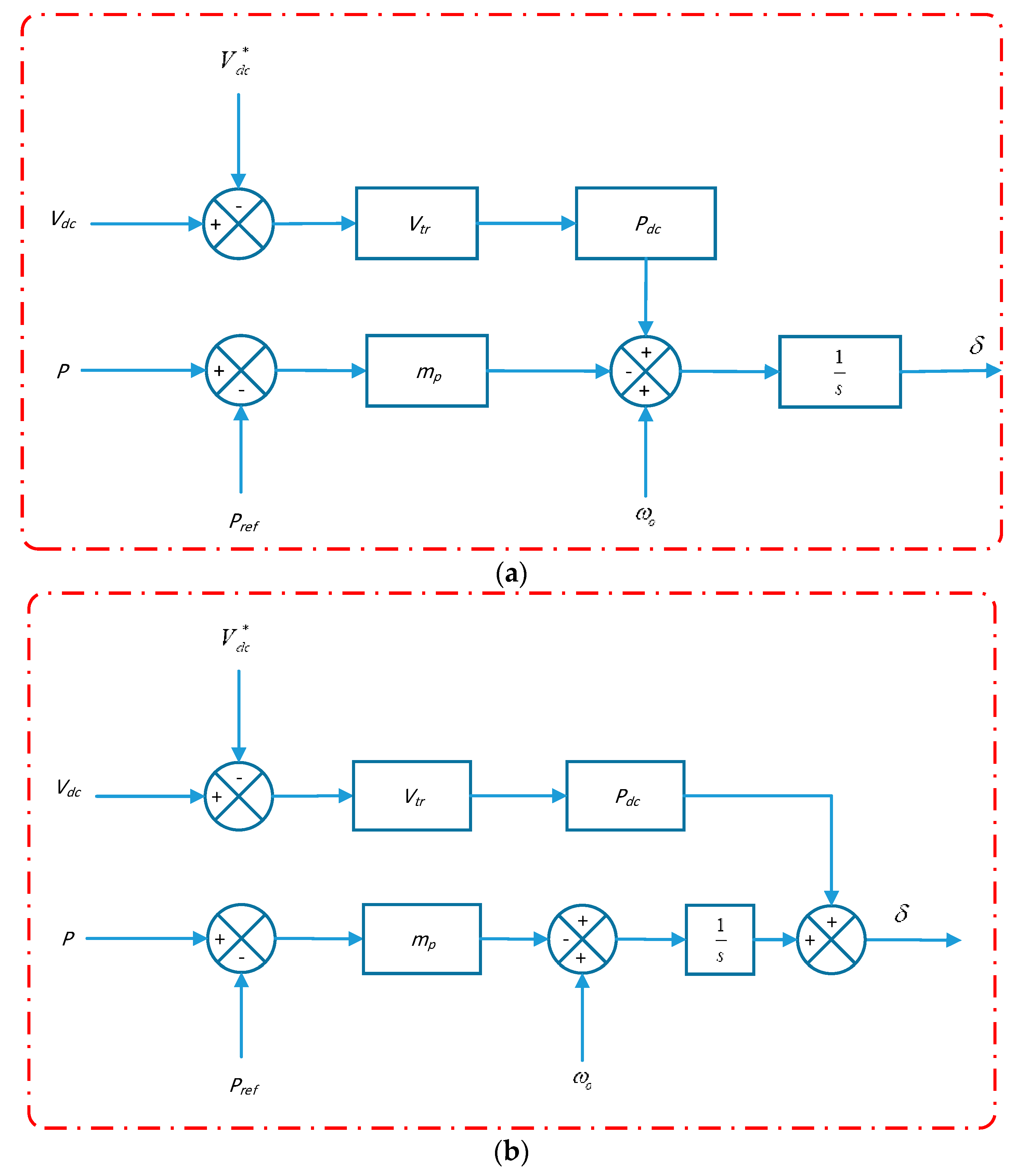
To limit voltage of DC link during the normal operation of a microgrid, the DC-link voltage after exceeding a triggering value ($V_{tr}$) will affect the frequency state which influences the active power.

To assure stable responses among hybrid microgrid networks in normal operations, Figure 17 describes two new control method proposals. When the voltage of DC-link surpasses a triggering value, the $V_{tr}$, a loop is started. This supplementary loop influences either the (a) phase state or (b) the frequency. In this research, an investigation is conducted to determine the state that has key effect on DC-link voltages. In this way, the controller effort needed to control the DC link voltage and use smaller control gains, which in turn preserves stability.

Through analysis of the first control track, as shown in Figure 17a, wherein controller output signaling is used to manipulate frequency state, the small-signal output frequency described in Equation (1) is thereby derived:

$$\Delta \omega =-m_p\times \Delta P+P_{dc}\times \Delta v_{dc}$$

(44)

where in $\Delta V_{dc}$ represents the smaller signal state of voltage DC-link, which is derived as:

$$\Delta V_{dc}=-\frac{k_{dc}}{s}\times \Delta p_{ins}$$

(45)

where $K_{dc}$ is the linearizing factor of the DC voltage and the negative sign indicates the negative flow of power. In the assumption that instantaneous and average powers are equal and through substitution of Equation (45) for Equation (44), we derive Equation (46):

$$\Delta \omega =-(m_p+\frac{P_{dc}\times K_{dc}}{s})\times \Delta P$$

(46)

Therefore, the phase state is obtained as Equation (47):

$$\Delta \delta =-(\frac{m_{p}s+P_{dc}\times K_{dc}}{s^2})\times \Delta P$$

(47)

For the control system shown in Figure 17b, the frequency and phase-states are as follows:

$$\Delta \omega =-(m_{p}s+P_{dc}\times K_{dc})\times \Delta P$$

(48)

$$\Delta \delta =-[\frac{m_{p}s+P_{dc}\times K_{dc}}{s}]\times \Delta P$$

(49)

An evaluation of Equation (46) with Equation (48) shows that the technique demonstrated in Figure 17a operates as the Proportional Integral ($PI$) controller of the output power. However, this approach may not offer faster action against introduced power. Conversely, the technique demonstrated in Figure 17b operates as the proportional derivative ($PD$) controller. In this approach, the power derivative is not applied directly, although the action is realized in the proposed loop. The derivative term is well-known for providing the fastest response needed for limiting any introduced DC-link voltage and power rises. Additionally, when compared to Equation (49), an added pole is obtained at origin in Equation (47), thereby introducing a ${90}^{\mathrm{o}}$ phase lag that results in lower stability margins. In accord with the above discussions, the technique demonstrated in Figure 17b is shown to perform better overall.

8. Analysis of the Participation Factor

Participation analysis was performed to attain further insight into the excellence of the technique, as indicated in Figure 17b, over that demonstrated in Figure 17a. The participation factor $P_{ki}$ in Equation (50) of eigenvalues on a state represents a measure of the influence of the state regarding the eigenvalue. Conversely, the participation factor ${\pi }_{ki}$ in Equation (51) of eigenvalues on a state represents a measure of whichever mode forms the majority of the response.

$$P_{ki}=r_{ki}\times l_{ki}$$

(50)

$${\pi }_{ki}=\frac{{\left[Re\left(l_{ki}\right)\right]}^2}{Re\left(l_{ki}\right)\times {\left[Re\left(l_{ki}\right)\right]}^T}$$

(51)

where $k$ denotes the $k_{th}$ state, $i$ denotes the $i_{th}$ mode. The eigenvalues for the system are calculated from Equation (43) as in

Table 4. The eigenvalues of the microgrid system.

Eigenvalues	Locations	Eigenvalues	Locations
${\lambda }_1$	0.0	${\lambda }_{14}$	−151 + 318 i
${\lambda }_2$	0.0	${\lambda }_{15}$	−151 − 318 i
${\lambda }_3$	0.0	${\lambda }_{16}$	−90 + 318 i
${\lambda }_4$	−224,683,637 + 316 i	${\lambda }_{17}$	−90 − 318 i
${\lambda }_5$	−224,683,637 − 316 i	${\lambda }_{18}$	−4
${\lambda }_6$	−224,683,637 + 316 i	${\lambda }_{19}$	−6
${\lambda }_7$	−224,683,637 − 316 i	${\lambda }_{20}$	−20 + 7 i
${\lambda }_8$	−2,546,836 + 316 i	${\lambda }_{21}$	−20 − 7 i
${\lambda }_9$	−2,546,836 − 316 i	${\lambda }_{22}$	−23
${\lambda }_{10}$	−693,417 + 316 i	${\lambda }_{23}$	−25
${\lambda }_{11}$	−693,417 − 316 i	${\lambda }_{24}$	−31
${\lambda }_{12}$	−31,719 + 316 i	${\lambda }_{25}$	−31
${\lambda }_{13}$	−31,719 − 316 i	${\lambda }_{26}$	0

.

As the aim is to control the DC voltage state variable, we are looking for modes with key effects on the active power P state variable, given the direct relationship of $P$ with DC-link voltage.

Table 5. State participation variables of dominant modes.

Mode/State	$\Delta {\mathit{\delta }}_1$	$\Delta {\mathit{P}}_1$	$\Delta {\mathit{\delta }}_2$	$\Delta {\mathit{P}}_2$	$\Delta {\mathit{\delta }}_3$	$\Delta {\mathit{P}}_3$
${\lambda }_{20,21}$	0.34	0	0.64	0	0.03	0
${\lambda }_{23}$	0.34	0	0.03	0	0.61	0
${\lambda }_{25}$	1.01	0	0	0	0	0

describes participation factors for eigenvalues on the system states. Eigen values ${\lambda }_{20}{\lambda }_{21}{\lambda }_{23}{\lambda }_{25}$ retain dominant influence on power responses. Operation of these modes can rework the active power response through transients, and thus, DC connection voltages can be reduced. Further analysis of the factor of participation is carried out to determine which states have key effects on these modes. Although the frequency is not a direct state, it includes a power output via a scalar function in relation to the power state as stated in Equation (11). Thus,

Table 6. Phase/power participation factors in selected modes.

State	${\mathit{\lambda }}_{14,15}$	${\mathit{\lambda }}_{16,17}$	${\mathit{\lambda }}_{18}$	${\mathit{\lambda }}_{19}$	${\mathit{\lambda }}_{20,21}$	${\mathit{\lambda }}_{22}$	${\mathit{\lambda }}_{23}$	${\mathit{\lambda }}_{24}$	${\mathit{\lambda }}_{25}$
$\Delta {\delta }_1$	0	0	0	0	0	0	0	0	0
$\Delta P_1$	0.002	0	0.07	0.1	0.2	0.1	0.6	0.1	0.5
$\Delta Q_1$	0.008	0	0	0.07	0.1	0.42	0.09	0.5	0.07
$\Delta io{d}_1$	0.1	0	0	0	0	0	0	0	0
$\Delta io{q}_1$	0.1	0	0	0	0	0	0	0	0
$\Delta {\delta }_2$	0.001	0	0.08	1.2	0.5	0	0.03	0	0
$\Delta P_2$	0	0	0.01	0.2	0.5	0	0.07	0.01	0.35
$\Delta Q_2$	0.014	0	0	0.14	0.2	0	0.01	0.3	0.07
$\Delta io{d}_2$	0.2	00	0	0	0	0	0	0	0
$\Delta io{q}_2$	0.2	0	0	0.009	0	0	0	0	0
$\Delta {\delta }_3$	0	0	1.3	0.083	0.04	0.15	0.45	0	0
$\Delta P_3$	0	0	0.16	0.017	0.04	0.26	1	0.1	0.5
$\Delta Q_3$	0.001	0	0	0.01	0.017	0.77	0.18	0.4	0.07
$\Delta io{d}_3$	0.016	0.11	0	0	0	0	0	0	0
$\Delta io{q}_3$	0.016	0.11	0	0	0	0	0	0	0
$\Delta iolin{e}_{D1}$	0.1	0.07	0	0	0	0	0	0	0
$\Delta iolin{e}_{Q1}$	0.1	0.2	0	0	0	0	0	0	0
$\Delta iolin{e}_{D2}$	0.03	0.2	0	0	0	0.01	0	0	0
$\Delta iolin{e}_{Q2}$	0.03	0	0	0	0	0.01	0	0	0
$\Delta ioloa{d}_{D1}$	0	0	0	0	0	0	0	0	0
$\Delta ioloa{d}_{Q1}$	0	0	0	0	0	0	0	0	0
$\Delta ioloa{d}_{D2}$	0	0	0	0	0	0	0	0	0
$\Delta ioloa{d}_{Q2}$	0	0	0	0	0	0	0	0	0
$\Delta vd{c}_1$	0	0	0	0	0	0	0	0	0
$\Delta vd{c}_2$	0	0	0	0	0	0	0	0	0
$\Delta vd{c}_3$	0	0	0	0	0	0	0	0	0

describes the phase and participation of the power state in the modes investigated, as was established early on. The results indicate that phase state has greater effect than power state on mode, which works to shape output power and consequently DC-link voltage. This validates similar conclusions made in the last section, in that the method displayed in Figure 17b performs better than that displayed in Figure 17a, for it results in smaller controller gains required to effect similar actions.

9. The Controller Design

After consideration of the method described in Figure 17b, and by perturbing Equation (1) and then computing the phase state variable, we derive:

$$\Delta \delta =\frac{\Delta \omega }{s}+P_{dc}\times \Delta v_{dc}$$

(52)

$$S\Delta \delta =-m_p\Delta P-P_{dc}\times k_{dc}\times \Delta P_{ins}$$

(53)

Equation (53) has been used in the Equation scheme state-space matrix Equation (43), wherein $\Delta P$ and $\Delta P_{ins}$ are redefined. Figure 18 describes eigenvalue when proposed control gain varies as follows: $0.0001P_{dc}$ $0.002$.

From Figure 18, we can see following:

• The increase in the proposed gain of control ($P_{dc})$ affects targeted eigenvalues ${\lambda }_{20}$, ${\lambda }_{21}$, ${\lambda }_{23}$, in alignment with that displayed in Table 6. Nevertheless, certain other eigenvalues are similarly affected, namely ${\lambda }_{14}$, ${\lambda }_{15}$, ${\lambda }_{16}$, ${\lambda }_{17}$, as couplings between eigenvalues and state variables cannot be easily analysed. In addition, the targeted ${\lambda }_{25}$ demonstrates negligible change, for it is mostly subject to determining filter bandwidth, in which ${\lambda }_{18}$, ${\lambda }_{19}$, ${\lambda }_{24}$, are not influenced.
• Increased $P_{dc}$ movement targets eigenvalues farther to the left and therefore increases damping of system. Nevertheless, high frequency eigenvalue similarly move towards imaginary axis, whereby at certain higher gains, system instability ensues.

10. Simulation Results

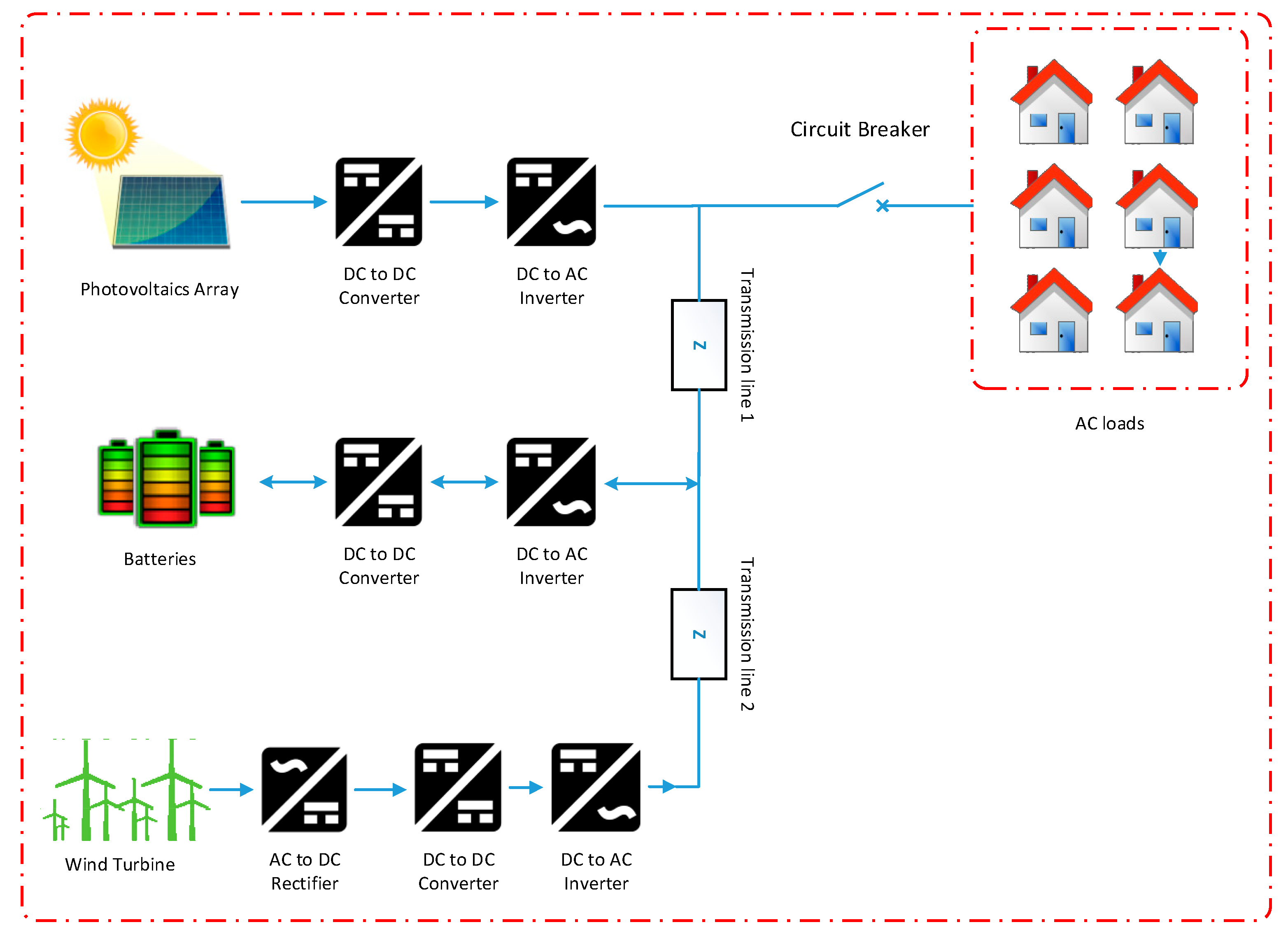
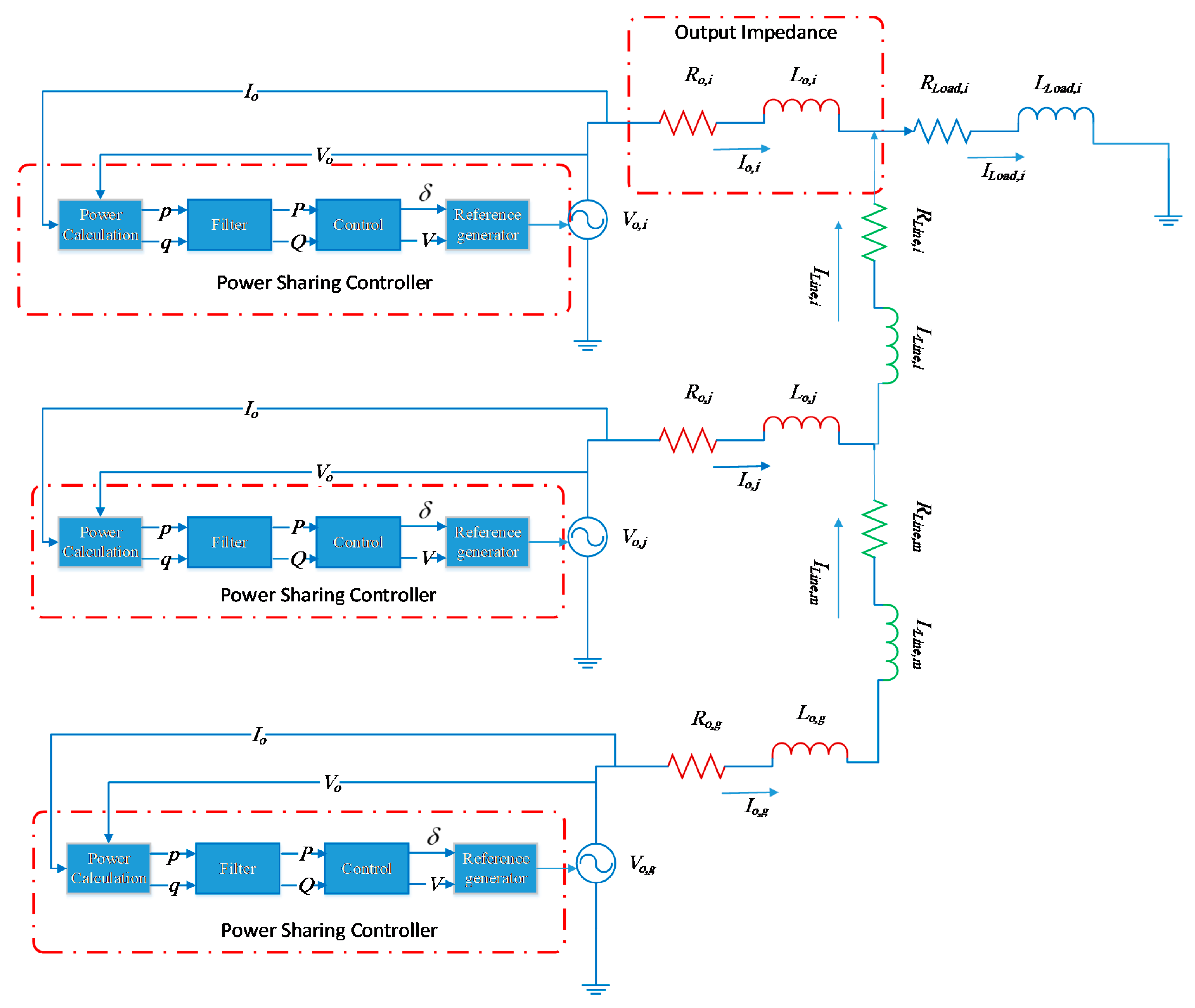
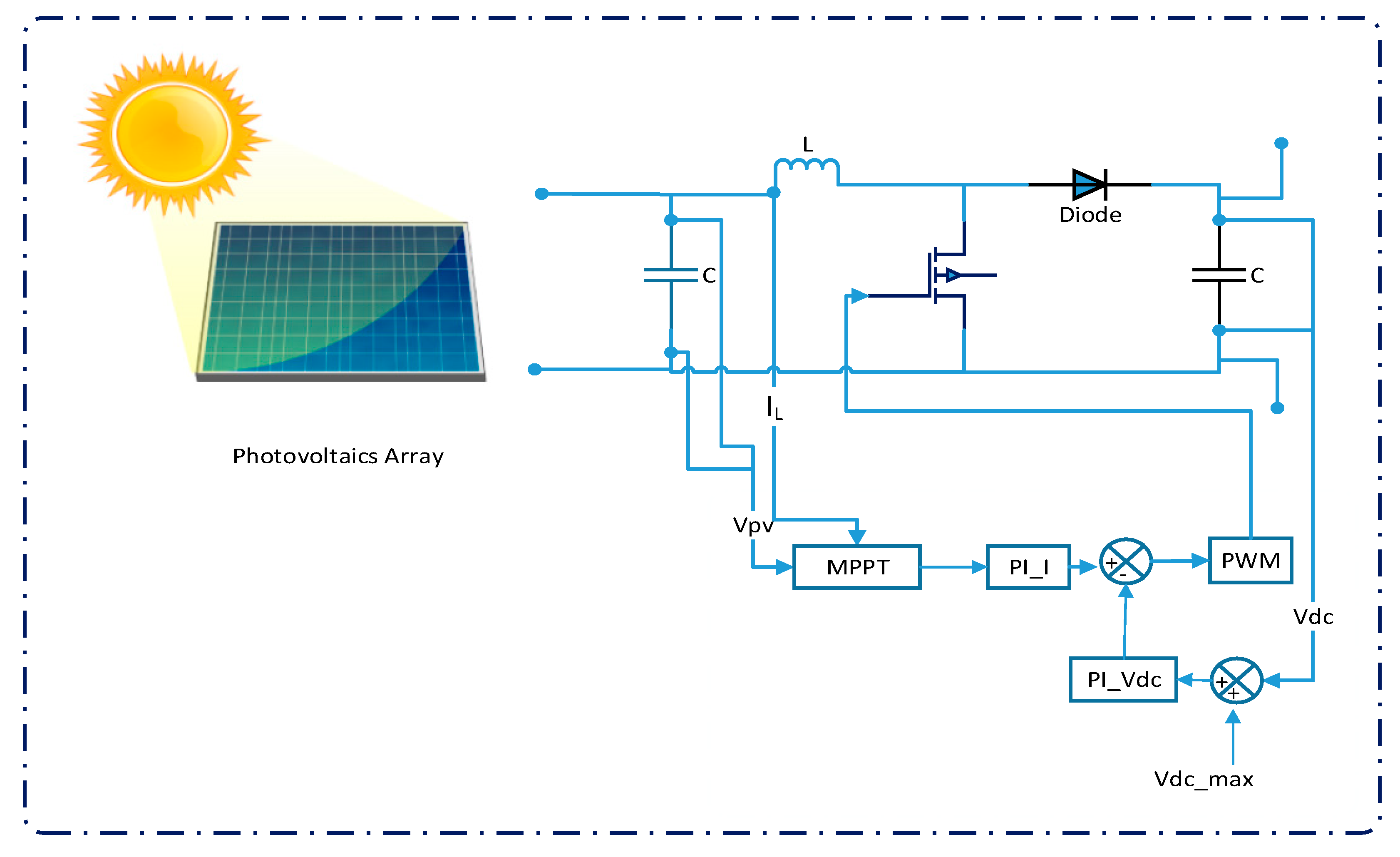
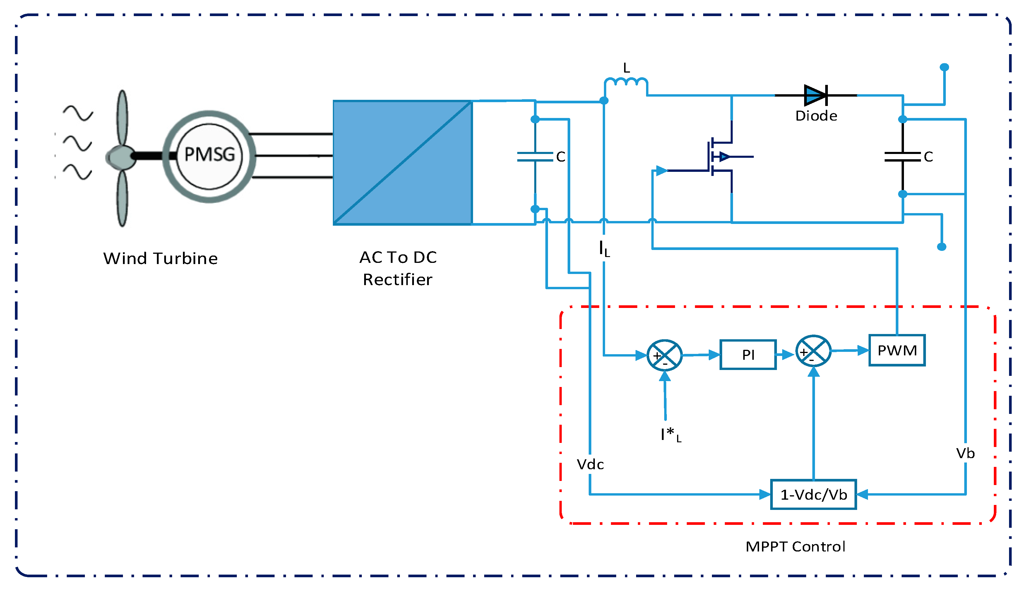
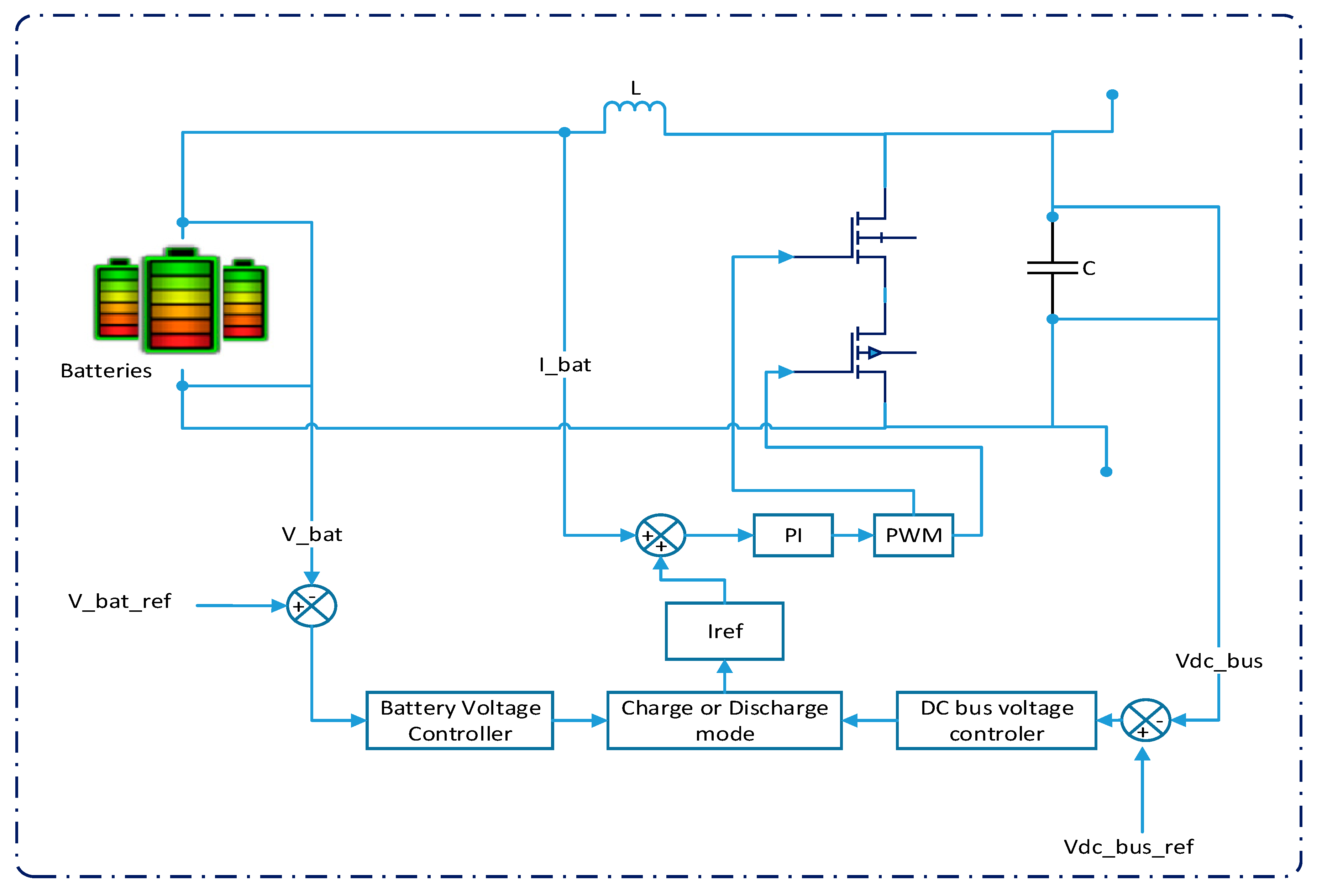
The suggested hybrid microgrid network comprising three inverters, as displayed in Figure 1 in SimPowerSystem, is simulated in order to confirm the performance of the suggested control strategy. Inverters and converters are characterized in models of renewable energy source, as photovoltaics, wind turbines, and batteries. The parameters of the simulation are given in

Table 7. The parameters of the system.

Symbols	Descriptions	Values
$L_{o,i}$$R_{o,i}$	Output impedance of inverter	$1\mathrm{mH}$, $1\times {10}^{-1}$ Ω
$L_{line,1}$, $R_{line,1}$	Impedance of line1	$1\mathrm{mH}$, $2\times {10}^{-3}$ Ω
$L_{line,2}$, $R_{line,2}$	Impedance of line2	$2\mathrm{mH}$, $3\times {10}^{-3}$ Ω
$m_p$	Droop gain frequency	10-3 rad/s
$n_q$	Droop gain voltage	${10}^{-3}$
$V_o$	Set point voltage	110 Vrms
$f_o$	Set point frequency	50 Hz
${\omega }_c$	Cut off frequency of filter	$30\mathrm{rad/s}$
$V_{DC-Link}$	Voltage of DC link	200 V
$V_{trip}$	Trip voltage of DC link	280 V
$V_{tr}$	Voltage of Triggering	215 V
$K_{dc}$	Linearization factor	$2.4$
$C_{dc\_link}$	Capacitor of Dc-Link	2 mF
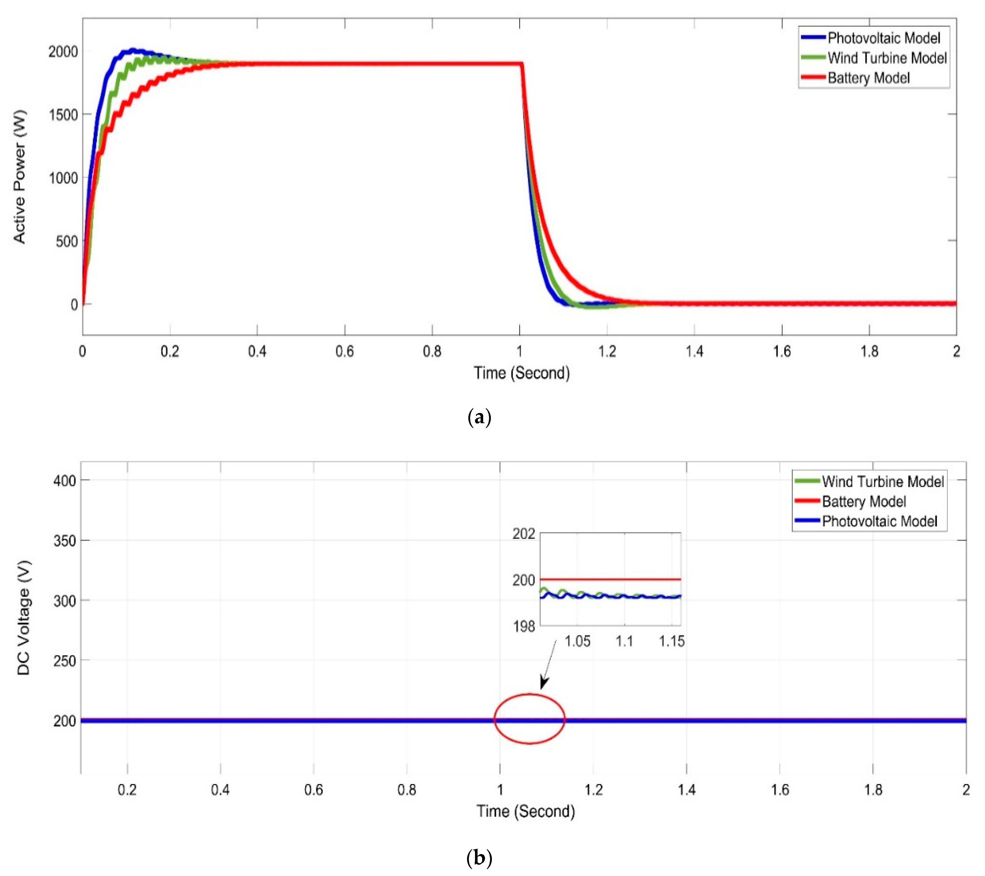
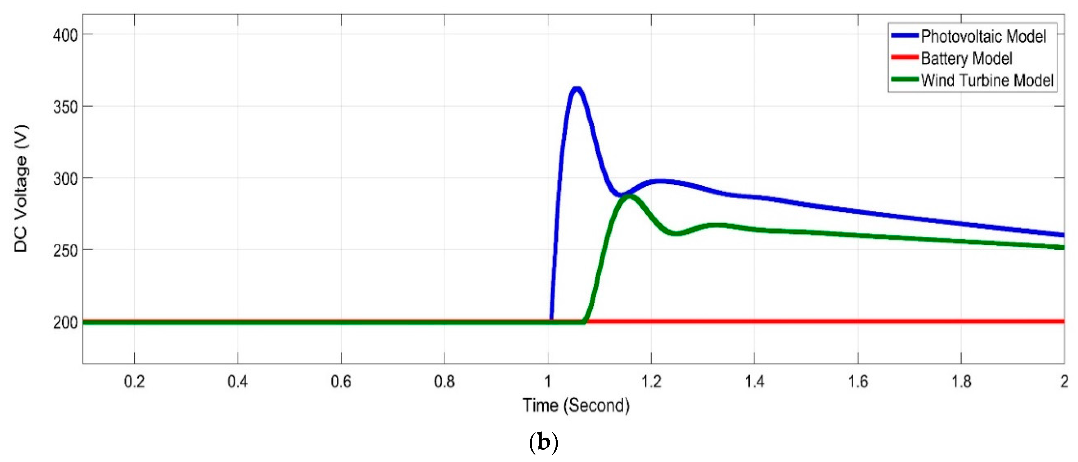
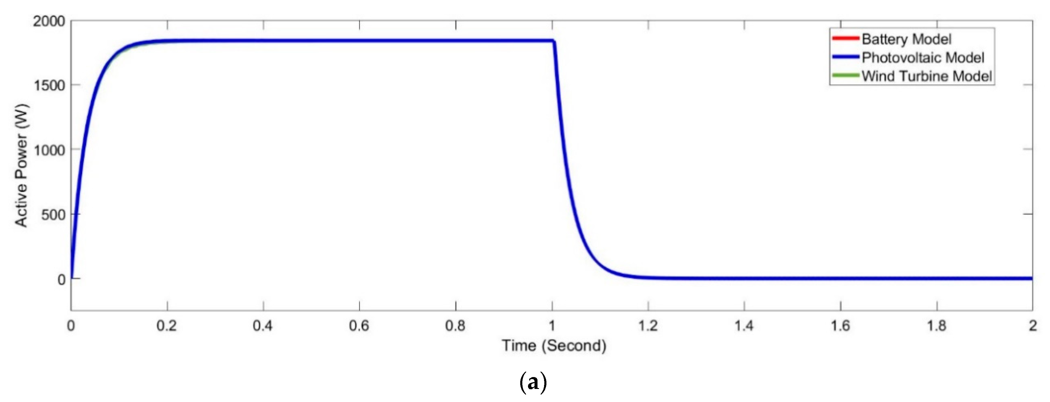
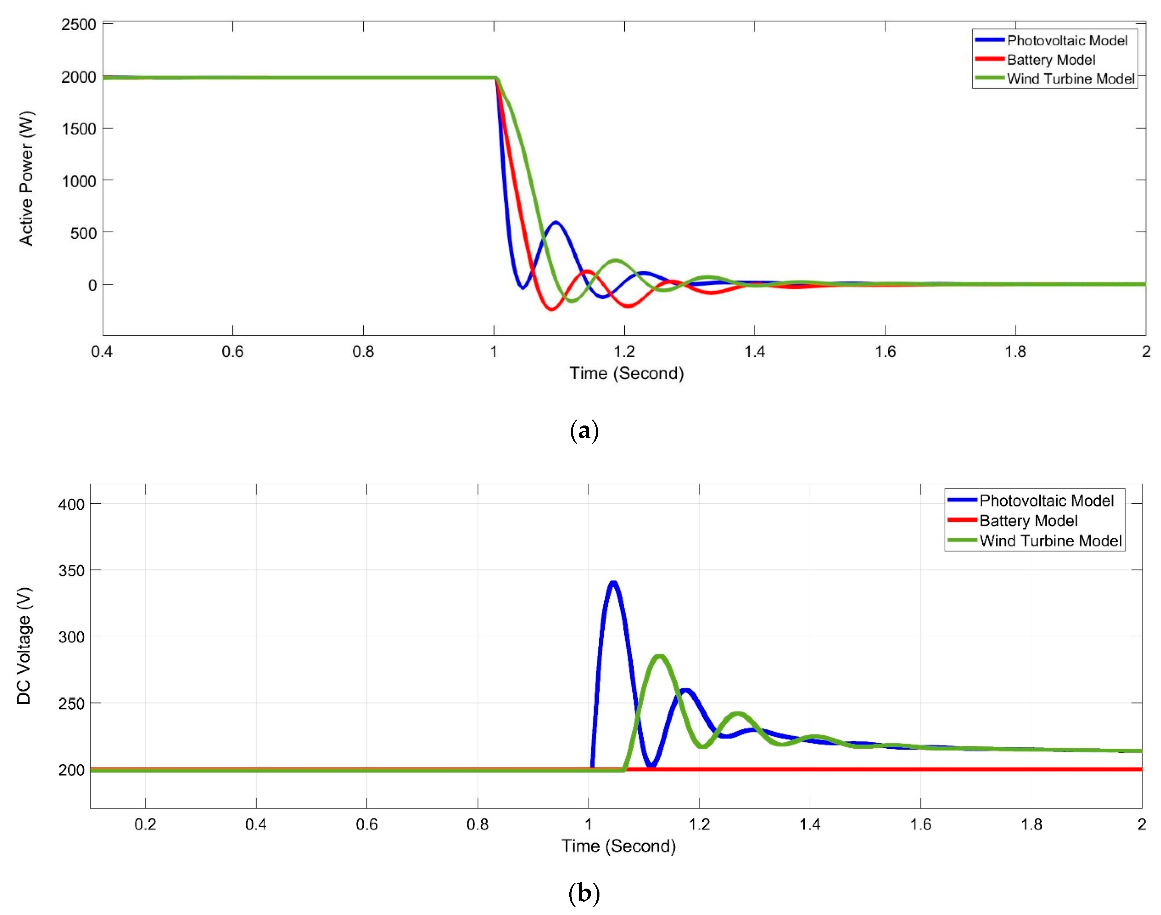
$P_{dc}$	Controller gain	5 × ${10}^{-4}$

. DC-link voltage is acquired whenever loads instantaneously change from 100% of 6 kW down to 0%, with the resulting power response displayed in Figure 19a. Clearly, the response remains well-damped due to the performance of the proposed controller that activates automatically whenever DC voltage rises above $V_{tr}$. This result is worthy of comparison as shown in Figure 13, which represents the same system except that the controller is not activated. Furthermore, DC-link voltage in Figure 19b is constrained and remains below trip levels, which validates the efficiency of the suggested approach.

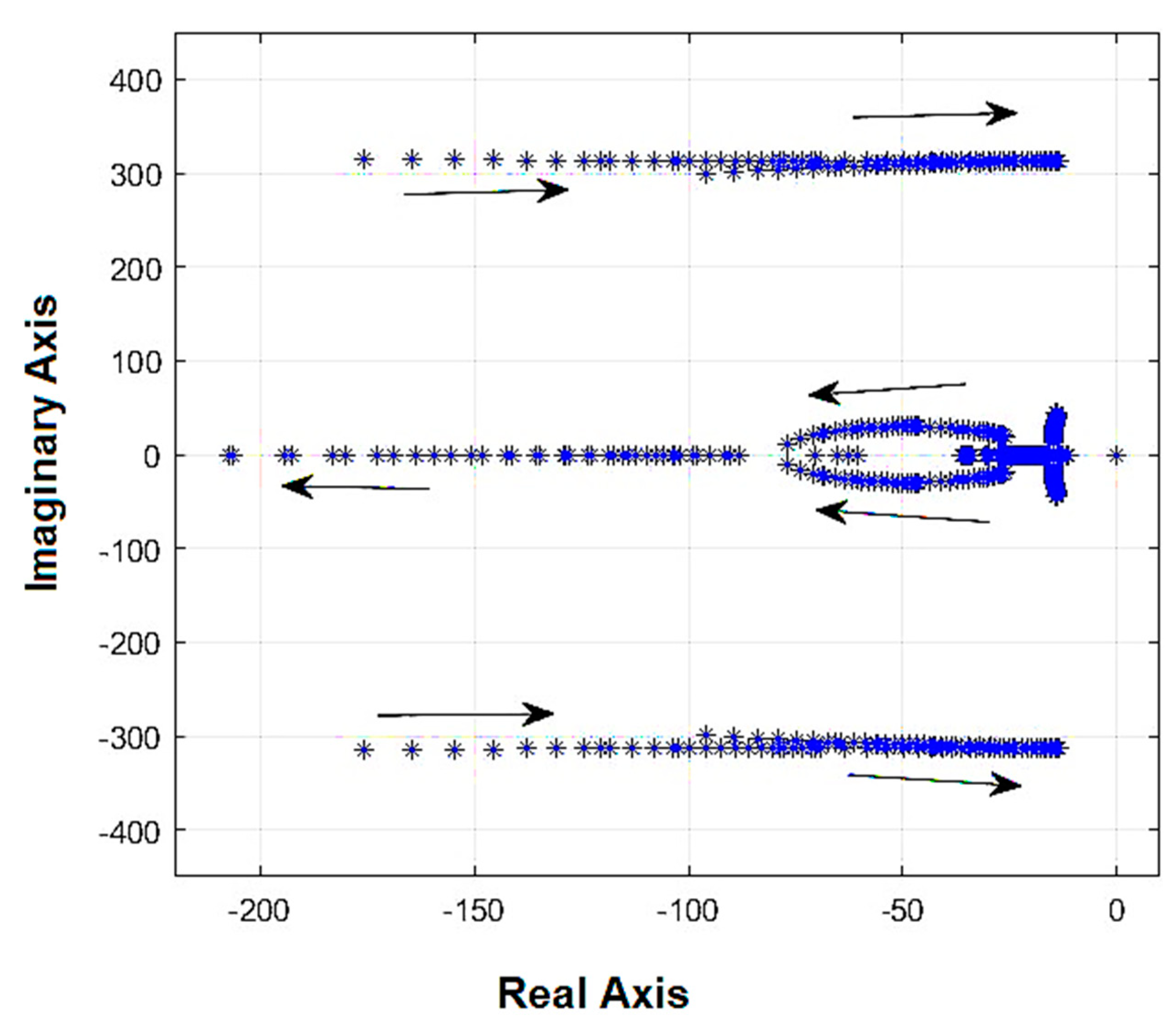
Figure 20 illustrates average active energy and response of DC voltage when proposed controller’s gain is P_dc = 0.001. The system is unstable and oscillation frequency is 314 rad/second, this is consistent with the prediction in Figure 18 as the system becomes unstable and oscillation frequency is 312 rad/second.

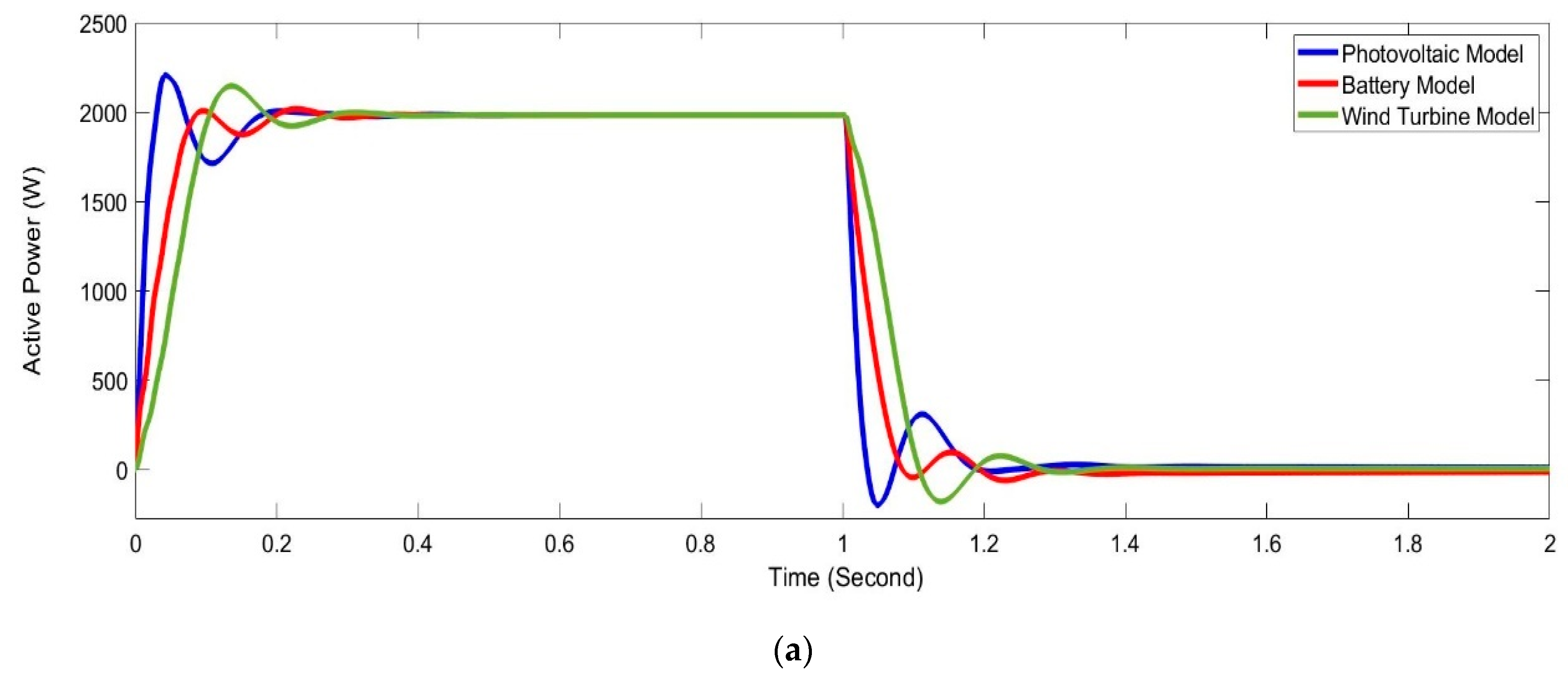
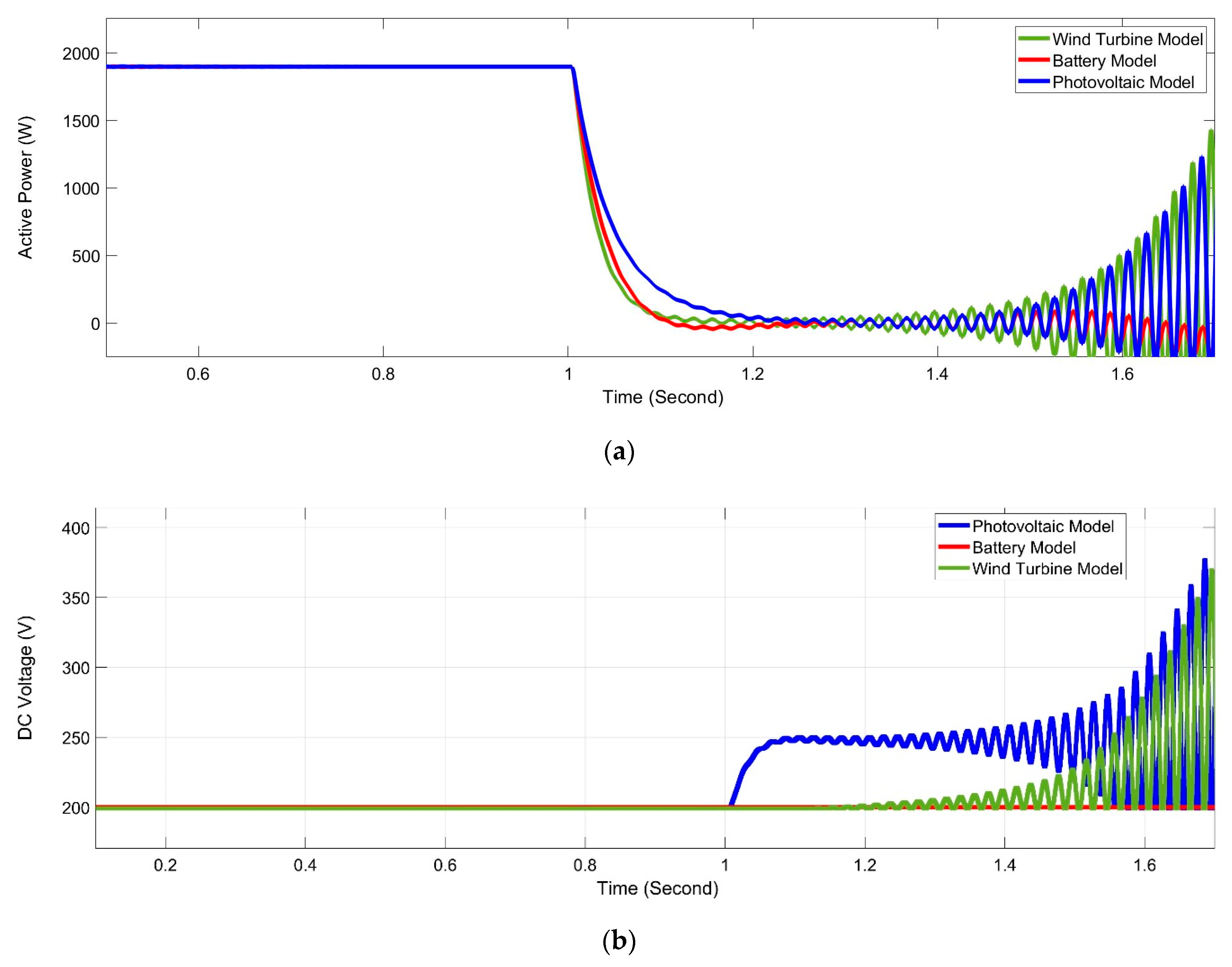
To validate the recommended approach in view of the excellence of technique indicated in Figure 17b over that demonstrated in Figure 17a, Figure 21 describes response when control method, as displayed in Figure 17a, is implemented with $P_{dc}=0.005$. The gain was selected for its similar capacity to tuning DC-link voltage, as illustrate in Figure 19b. Clearly, the gain exceeds that used in the suggested method, as shown in Figure 17b, which therefore confirms that the suggested method requires less effort in regulating DC voltage. Furthermore, DC-link and power voltage responses can be highly oscillatory in comparison to that described in Figure 19.

11. Conclusions

This research investigated the effect of mismatched line impedances on the stability of DC-link voltages under sudden load changes, as well as the performance of parallel inverters operating in hybrid microgrids. Studies showed that comparable droop gains do not assure similar power responses during transients in every case. If an appreciable line impedance mismatch exists, circulating power transients may degrade stability. The suggested technique was found to perform more efficiently than the frequency loop approach in stabilizing DC-link voltage states in microgrids. Any stable-state errors appeared solely during instances of zero-load transition. Nevertheless, this does not present a major issue when the load reconnects, as the level is sufficient to discharge the excess energy and thereby maintains zero error. The results of the simulation demonstrated also the improved performance and effectiveness of the suggested control approach. Additionally, the suggested control strategy exhibited much robustness against larger load variations. Furthermore, in an effort to avert the drawbacks of standard droop control, an enhanced droop control strategy derived from integrator current-sharing was developed. The MPPT method was used in both wind turbine and photovoltaic stations towards extracting maximum amounts of power from such hybrid power systems.

The new strategy aimed to unify the control loops for all inverters in each mode of operation and for different energy sources to be DC-voltage regulators. This structure immunized the stability of the DC-link voltage states and the overall reliability of the microgrid against sudden unplanned islanding. The control scheme was analyzed and tested by simulation. As future works, the following points are suggested: (I) implementing the presented strategy on a real network and comparing the results (II) the proposed control scheme can be extended to address the network-related issues, such as data loss, packet jamming, link failure, cyber-attack, etc., using a cyber-physical systems framework.

References

1. Anvari-Moghaddam, A.; Seifi, A.R. A Comprehensive Study on Future Smart Grids: Definitions, Strategies and Recommendations. J. North Carol. Acad. Sci. 2011, 127, 28–34. [Google Scholar]
2. Frances, A.; Anvari-Moghaddam, A.; Rodriguez-Diaz, E.; Vasquez, J.C.; Guerrero, J.M.; Uceda, J. Dynamic Assessment of COTS Converters-based DC Integrated Power Systems in Electric Ships. IEEE Trans. Ind. Inf. 2018, 13, 5518–5529. [Google Scholar] [CrossRef] [Green Version]
3. Colak, I.; Kabalci, E.; Fulli, G.; Lazarou, S. A survey on the contributions of power electronics to smart grid systems. Renew. Sustain. Energy Rev. 2015, 47, 45–57. [Google Scholar] [CrossRef]
4. Mavrokefalidis, C.; Ampeliotis, D.; Berberidis, K. A study of the communication needs in micro-grid systems. In Proceedings of the IEEE General Assembly and Scientific Symposium of the International Confinernce Union of Radio Science (URSI GASS), Montreal, QC, Canada, 19–26 August 2017; Volume 6, pp. 19–26. [Google Scholar] [CrossRef]
5. Tran, T.S.; Nguyen, D.T.; Fujita, G. The Analysis of Technical Trend in Islanding Operation, Harmonic Distortion, Stabilizing Frequency, and Voltage of Islanded Entities. Resources 2019, 8, 14. [Google Scholar] [CrossRef] [Green Version]
6. Heydari, R.; Khayat, Y.; Naderi, M.; Anvari-Moghaddam, A.; Dragicevic, T.; Blaabjerg, F. A Decentralized Adaptive Control Method for Frequency Regulation and Power Sharing in Autonomous Microgrids. In Proceedings of the 28th International Symposium on Industrial Electronics (ISIE), Vancouver, BC, Canada, 12–14 June 2019. [Google Scholar] [CrossRef]
7. Moradzadeh, A.; Sadeghian, O.; Pourhossein, K.; Mohammadi-Ivatloo, B.; Anvari-Moghaddam, A. Improving Residential Load Disaggregation for Sustainable Development of Energy via Principal Component Analysis. Sustainability 2020, 12, 3158. [Google Scholar] [CrossRef] [Green Version]
8. Peyghami, S.; Mokhtari, H.; Blaabjerg, F. Autonomous Operation of a Hybrid AC/DC Microgrid with Multiple Interlinking Converters. IEEE Trans. Smart Grid 2018, 9, 6480–6488. [Google Scholar] [CrossRef] [Green Version]
9. Baharizadeh, M.; Karshenas, H.R.; Guerrero, J.M. Control Strategy of Interlinking Converters as the Key Segment of Hybrid AC–DC Microgrids. IET Gen. Trans. Dist. 2016, 10, 1671–1681. [Google Scholar] [CrossRef] [Green Version]
10. Nejabatkhah, F.; Li, Y.W. Overview of Power Management Strategies of Hybrid AC/DC Microgrid. IEEE Trans. Power Electron. 2015, 30, 7072–7089. [Google Scholar] [CrossRef]
11. Mohiti, M.; Monsef, H.; Anvari-Moghaddam, A.; Lesani, H. Two-Stage Robust Optimization for Resilient Operation of Microgrids Considering Hierarchical Frequency Control Structure. IEEE Trans. Ind. Electron. 2019, 35, 1256–1265. [Google Scholar] [CrossRef]
12. Dragičević, T.; Lu, X.; Vasquez, J.C.; Guerrero, J.M. DC microgrids—Part I: A Review of Control Strategies and Stabilization Techniques. IEEE Trans. Power Electron. 2016, 31, 4876–4891. [Google Scholar] [CrossRef] [Green Version]
13. Loh, P.C.; Li, D.; Chai, Y.K.; Blaabjerg, F. Autonomous operation of hybrid microgrid with AC and DC subgrids. IEEE Trans. Power Electron 2016, 28, 2214–2223. [Google Scholar] [CrossRef]
14. Faria, J.; Pombo, J.; Calado, M.D.R.; Mariano, S. Power Management Control Strategy Based on Artificial Neural Networks for Standalone PV Applications with a Hybrid Energy Storage System. Energies 2019, 12, 902. [Google Scholar] [CrossRef] [Green Version]
15. Vahedipour-Dahraie, M.; Rashidizadeh-Kermani, H.; Anvari-Moghaddam, A.; Guerrero, J.M. Stochastic Risk-Constrained Scheduling of Renewable-Powered Autonomous Microgrids with Demand Response Actions: Reliability and Economic Implications. IEEE Trans. Ind. Appl. 2019, 56, 1882–1895. [Google Scholar] [CrossRef]
16. Hemmati, M.; Mohammadi-Ivatloo, B.; Abapour, M.; Anvari-Moghaddam, A. Optimal Chance-Constrained Scheduling of Reconfigurable Microgrids Considering Islanding Operation Constraints. IEEE Syst. J. 2020, 26. [Google Scholar] [CrossRef]
17. Anvari-Moghaddam, A.; Mohammadi-Ivatloo, B.; Asadi, S.; Guldstrand Larsen, K.; Shahidehpour, M. Sustainable Energy Systems Planning, Integration, and Management. Appl. Sci. 2019, 9, 4451. [Google Scholar] [CrossRef] [Green Version]
18. Khorsandi, A.; Ashourloo, M.; Mokhtari, H. A Decentralized Control Method for A Low-Voltage DC Microgrid. IEEE Trans. Energy Convers. 2014, 29, 793–801. [Google Scholar] [CrossRef]
19. Farzin, H.; Fotuhi-Firuzabad, M.; Moeini-Aghtaie, M. Stochastic Energy Management of Microgrids during Unscheduled Islanding Period. IEEE Trans. Ind. Inf. 2016, 13, 1079–1087. [Google Scholar] [CrossRef]
20. Battistelli, C.; Agalgaonkar, Y.P.; Pal, B.C. Probabilistic Dispatch of Remote Hybrid Microgrids Including Battery Storage and Load Management. IEEE Trans. Smart Grid 2016, 8, 1305–1317. [Google Scholar] [CrossRef]
21. Chen, Q.; Xu, Q.; Wu, C. Optimal Sharing Strategies of Idle Manufacturing Resource Considering the Effect of Supply-Demand Matching. In Proceedings of the 2019 International Conference on Industrial Engineering and Systems Management (IESM), Shanghai, China, 25–27 September 2019; pp. 6480–6488. [Google Scholar] [CrossRef]
22. Shafiee, Q.; Guerrero, J.M.; Vasquez, J.C. Distributed Secondary Control for Island Microgrids—A Novel Approach. IEEE Trans. Power Electron. 2015, 29, 1018–1031. [Google Scholar] [CrossRef] [Green Version]
23. Khan, M.Z.; Khan, M.M.; Jiang, H.; Hashmi, K.; Shahid, M.U. An Improved Control Strategy for Three-Phase Power Inverters in Islanded AC Microgrids. Inventions 2018, 3, 47. [Google Scholar] [CrossRef] [Green Version]
24. Ma, J.; Wang, X.; Liu, J.; Gao, H. An Improved Droop Control Method for Voltage-Source Inverter Parallel Systems Considering Line Impedance Differences. Energies 2019, 12, 1158. [Google Scholar] [CrossRef] [Green Version]
25. He, J.; Li, Y.W. Hybrid voltage and current control approach for DG-grid interfacing converters with LCL filters. IEEE Trans. Ind. Electron. 2015, 60, 1797–1809. [Google Scholar] [CrossRef]
26. Gupta, Y.; Chatterjee, K.; Doolla, S. A Simple Control Scheme for Improving Reactive Power Sharing in Islanded Microgrid. IEEE Trans. Power Syst. 2020, 1079–1087. [Google Scholar] [CrossRef]
27. Zhang, C.; Guerrero, J.M.; Vasquez, J.C.; Coelho, E.A.A. Control Architecture for Parallel-Connected Inverters in uninterruptible Power Systems. IEEE Trans. Power Electron. 2016, 31, 5176–5188. [Google Scholar] [CrossRef] [Green Version]
28. Cingoz, F.; Elrayyah, A.; Sozer, Y. Optimized Settings of Droop Parameters Using Stochastic Load Modeling for Effective DC Microgrids Operation. IEEE Trans. Ind. Appl. 2016, 53, 1358–1371. [Google Scholar] [CrossRef]
29. Liu, J.; Miura, Y.; Bevrani, H.; Ise, T. Enhanced Virtual Synchronous Generator Control for Parallel Inverters in Microgrids. IEEE Trans. Smart Grid 2017, 8, 2268–2277. [Google Scholar] [CrossRef]
30. Trinh, Q.N.; Wang, P.; Tang, Y.; Choo, F.H. Mitigation of DC and Harmonic Currents Generated by Voltage Measurement Errors and Grid Voltage Distortions in Transformer Less Grid-Connected Inverters. IEEE Trans. Energy Convers. 2018, 33, 801–813. [Google Scholar] [CrossRef]
31. Ranjbaran, A.; Ebadian, M. A Power Sharing Scheme for Voltage Unbalance and Harmonics Compensation in an Islanded Microgrid. Electron. Power Syst. Res. 2018, 155, 153–163. [Google Scholar] [CrossRef]
32. Ren, B.; Sun, X.; Chen, S.; Liu, H. A Compensation Control Scheme of Voltage Unbalance Using a Combined Three-Phase Inverter in an Islanded Microgrid. Energies 2018, 11, 2486. [Google Scholar] [CrossRef] [Green Version]
33. Rey, J.M.; Vergara, P.P.; Castilla, M.; Camacho, A.; Velasco, M.; Martí, P. Droop hierarchical control strategy for inverter-based AC microgrids. IET Power. Electron. 2019, 7, 1079–1087. [Google Scholar] [CrossRef]
34. Martí, P.; Velasco, M.; Martín, E.X.; de Vicuña, L.G.; Miret, J.; Castilla, M. Performance Evaluation of Secondary Control Policies with Respect to Digital Communications Properties in Inverter-Based Islanded Microgrids. IEEE Trans. Smart Grid 2018, 9, 2192–2202. [Google Scholar] [CrossRef] [Green Version]
35. Cheng, Z.; Duan, J.; Chow, M.Y. A Comparison of Advanced Microgrid Management Systems. IEEE Ind. Electron. Mag. 2018, 12, 6–24. [Google Scholar] [CrossRef]
36. Hou, X.; Sun, Y.; Lu, J.; Zhang, X.; Koh, L.H.; Su, M.; Guerrero, J.M. Distributed Hierarchical Control of AC Microgrid Operating in Grid-Connected, Islanded and Their Transition Modes. IEEE Access 2018, 6, 77388–77401. [Google Scholar] [CrossRef]
37. Miret, J.; García de Vicuña, J.L.; Guzmán, R.; Camacho, A.; Moradi Ghahderijani, M. A Flexible Experimental Laboratory for Distributed Generation Networks Based On Power Inverters. Energies 2017, 10, 1589. [Google Scholar] [CrossRef] [Green Version]
38. Walid, I.; Suleiman, S.; Mohammad, A. Hybrid Generators-based AC Microgrid Performance Assessment in Island Mode. IET Power Electr. 2019, 12, 1973–1980. [Google Scholar] [CrossRef] [Green Version]
39. Rey, J.M.; Martí, P.; Velasco, M.; Miret, J.; Castilla, M. Secondary Switched Control with No Communications for Islanded Microgrids. IEEE Trans. Ind. Electron. 2018, 64, 8534–8545. [Google Scholar] [CrossRef] [Green Version]
40. Hussaian Basha, C.; Rani, C.; Brisilla, R.M.; Odofin, S. Mathematical Design and Analysis of Photovoltaic Cell Using MATLAB/Simulink. In Soft Computing for Problem Solving; Advances in Intelligent Systems and Computing; Springer: Singapore, 2019; Volume 1048, pp. 711–726. [Google Scholar] [CrossRef]
41. Sangwongwanich, A.; Blaabjerg, F. Mitigation of Interharmonics in PV Systems with Maximum Power Point Tracking Modification. IEEE Trans. Power Electron. 2019, 34, 8279–8282. [Google Scholar] [CrossRef] [Green Version]
42. Rakhshan, M.; Vafamand, N.; Khooban, M.H.; Blaabjerg, F. Maximum Power Point Tracking Control of Photovoltaic Systems. A Polynomial Fuzzy Model-Based Approach. IEEE J. Emerg. Sel. Top. Power Electron. 2018, 6, 292–299. [Google Scholar] [CrossRef]
43. Subramaniyan, A.B.; Pan, R.; Kuitche, J.; TamizhMani, G. Quantification of Environmental Effects on PV Module Degradation: A Physics-Based Data-Driven Modeling Method. IEEE J. Photovolt. 2018, 8, 1289–1296. [Google Scholar] [CrossRef]
44. Elnounou, K.T. Design of GA Sugeno Fuzzy Controller for Maximum Power Point and Sun Tracking in Solar Array Systems. Master’s Thesis, The Islamic University, Gaza, Palestine, 2013. [Google Scholar] [CrossRef]
45. Fathima, A.H.; Palanisamy, K. Optimization in Microgrids with Hybrid Energy Systems—A Review. Renew. Sustain. Energy Rev. 2015, 45, 431–446. [Google Scholar] [CrossRef]
46. Hong, Y.Y.; Lai, Y.Z.; Chang, Y.R.; Lee, Y.D.; Lin, C.H. Optimizing Energy Storage Capacity in Islanded Microgrids Using Immunity-Based Multi objective Planning. Energies 2018, 11, 585. [Google Scholar] [CrossRef] [Green Version]
47. Kong, X.; Ma, L.; Liu, X.; Abdelbaky, M.A.; Wu, Q. Wind Turbine Control Using Nonlinear Economic Model Predictive Control over All Operating Regions. Energies 2020, 13, 184. [Google Scholar] [CrossRef] [Green Version]
48. Hossain, M.A.; Pota, H.R.; Hossain, M.J.; Haruni, A.M.O. Active Power Management in a Low-Voltage Islanded Microgrid. Int. J. Electron. Power Energy Syst. 2018, 98, 36–48. [Google Scholar] [CrossRef] [Green Version]
49. Shahnia, F.; Arefi, A. Eigenanalysis-Based Small Signal Stability of the System of Coupled Sustainable Microgrids. Int. J. Electron. Power Energy Syst. 2017, 91, 42–60. [Google Scholar] [CrossRef]
50. Wen, B.; Boroyevich, D.; Burgos, R.; Mattavelli, P.; Shen, Z. Inverse Nyquist Stability Criterion for Grid-Tied Inverters. IEEE Trans. Power Electron. 2017, 32, 1548–1556. [Google Scholar] [CrossRef]
51. Rowe, C.N.; Summers, T.J.; Betz, R.E.; Cornforth, D.J.; Moore, T.G. Arctan Power—Frequency Droop for Improved Microgrid Stability. IEEE Trans. Power Electron. 2015, 28, 3747–3759. [Google Scholar] [CrossRef]
52. Shuai, Z.; Sun, Y.; Shen, Z.J.; Tian, W.; Tu, C.; Li, Y.; Yin, X. Microgrid stability: Classification and a review. Renew. Sustain. Energy Rev. 2016, 58, 167–179. [Google Scholar] [CrossRef]
53. Walid, R.M.I. Improved Control Strategies for Droop-Controlled Inverter-Based Microgrid, Doctor of Philosophy in Renewable Energy; University of Exeter: Exeter, UK, 2015. [Google Scholar]
Figure 1. The proposed system structure.
Energies 13 03480 g001
Figure 2. Droop control structure.
Energies 13 03480 g002
Figure 3. (a) ω–P droop characteristics of a microgrid and (b) V–P droop characteristics of microgrid.
Energies 13 03480 g003
Figure 4. The equivalent circuit of photovoltaic cell.
Energies 13 03480 g004
Figure 5. Typical current and voltage curve of photovoltaic cell.
Energies 13 03480 g005
Figure 6. A typical current-voltage curve of the photovoltaic.
Energies 13 03480 g006
Figure 7. Power characteristic curve for a wind turbine.
Energies 13 03480 g007
Figure 8. Microgrid stability classification.
Energies 13 03480 g008
Figure 9. Thevenin equivalent model of an inverter.
Energies 13 03480 g009
Figure 10. A multi-inverter islanded microgrid.
Energies 13 03480 g010
Figure 11. The eigenvalues of system, 5 × 10⁻⁵ mp 5 × 10⁻³ where (a) lines inductances neglected, (b) when L_Line1 = 10−3 H and L_Line1 = 2 × 10⁻³ H.
Energies 13 03480 g011
Figure 12. Simulation of identical distribution lines are used, (a) inverters power response, (b) DC link voltage response under loads change.
Energies 13 03480 g012
Figure 13. Simulation of different distribution lines are used, (a) the inverters power response, (b) DC link voltage response under loads change.
Energies 13 03480 g013aEnergies 13 03480 g013b
Figure 14. MPPT control of boost converter.
Energies 13 03480 g014
Figure 15. The control of the WT converter.
Energies 13 03480 g015
Figure 16. Control scheme of battery energy storage.
Energies 13 03480 g016
Figure 17. Diagrams of proposed controller where (a) is frequency loop, and (b) is the phase loop.
Energies 13 03480 g017
Figure 18. The root locus of the proposed system.
Energies 13 03480 g018
Figure 19. Simulation of loads change, where (a) active power responses, (b) responses of DC-link voltage.
Energies 13 03480 g019aEnergies 13 03480 g019b
Figure 20. Simulation result, where (a) the averaged power response, (b) response of DC link voltage.
Energies 13 03480 g020
Figure 21. The method shown in Figure 17a is used, where (a) is the response of averaged power, (b) is the DC link voltage response.
Energies 13 03480 g021