Time-Splitting Coupling of WaveDyn with OpenFOAM by Fidelity Limit Identified from a WEC in Extreme Waves

Abstract

Survivability assessment is the complexity compromising Wave energy development. The present study develops a hybrid model aiming to reduce computational power while maintaining accuracy for survivability assessment of a Point-Absorber (PA) Wave Energy Converter (WEC) in extreme Wave Structure Interaction (WSI). This method couples the fast inviscid linear potential flow time-domain model WaveDyn (1.2, DNV-GL, Bristol, UK) with the fully nonlinear viscous Navier–Stokes Computational Fluid Dynamics (CFD) code OpenFOAM (4.2, OpenFOAM.org, London, UK). The coupling technique enables the simulation to change between codes, depending on an indicator relating to wave steepness identified as a function of the confidence in the linear model solution. During the CFD part of the simulation, the OpenFOAM solution is returned to WaveDyn via an additional load term, thus including viscous effects. Developments ensure a satisfactory initialisation of CFD simulation to be achieved from a ‘hot-start’ time, where the wave-field is developed and the device is in motion. The coupled model successfully overcomes identified inaccuracies in the WaveDyn code due to the inviscid assumption and the high computational cost of the OpenFOAM code. Experimental data of a PA response under extreme deterministic events (NewWave) are used to assess WaveDyn’s validity limit as a function of wave steepness, in order to validate CFD code and develop the coupling. The hybrid code demonstrates the applicability of WaveDyn validity limit and shows promising results for long irregular sea-state applications.

1. Introduction

Wave energy is a promising sector for sustainable low-carbon energy production. However, despite the efforts made in the last decade, uncertainties in wave energy performance and cost remain. In 2016, survivability assessment has been identified as the main WEC concern in the five years to come by the Collaborative Computational Project in Wave Structure Interaction (CCP-WSI) Working Group [1]. Numerical modelling can play a key role in the assessment of extreme responses that are necessary to the understanding of WEC capacity to survive extreme conditions.

WECs are subjected to complex hydrodynamics phenomena, such as slamming waves or green water effect. Numerical models that are based on the weakly simplified Navier–Stokes equations, assumed of ‘high-fidelity’ (Figure 1), are necessary to model such hydrodynamics and the interaction with the device, whereas numerical models of ‘lower fidelity’ (Figure 1) are restricted by the assumptions made on the fluid properties (e.g., inviscid, or small displacement) or the equations solving procedure (e.g., linear potential flow). Therefore, their use is debatable for survivability assessment of WEC, which, in the meantime, justifies the use of CFD models ([2,3,4], among others).

However, assumed high-fidelity codes like CFD are too time-consuming for routine design use in industry [1]. Codes of lower fidelity are used instead, although being based on major physical assumptions inducing concerning uncertainties, especially in surge and pitch [5]. Inaccurate estimations of extreme response often lead to conservative design decisions that lower the commercial viability of a device [6]. In addition, lower fidelity models were developed by the Oil and Gas and shipping industries. WECs differ to ships and platforms by their size (i.e., WECs are typically smaller) and their motion, which should be accentuated to generate power. Viscous effects tend to become more important for WECs, whereas diffraction and radiation effects tend to decrease. Hence, when radiation diffraction effects dominate viscous effects, Oil&Gas low-fidelity numerical models that are based on simplified physics remain reliable; whereas, when viscous effects dominate, high-fidelity numerical models, like CFD, are justified. During a given simulation—especially for a long irregular sea-state—the regime is likely to change from one to the other.

Uncertainties remain regarding which numerical model to use for a given application. At best, numerical models are classified, depending on the physical processes represented (i.e., wave-breaking, wave non-linearity) [7]. The absence of a parametric study function of a wave-parameter makes the choice of the selected model for survivability vague. For long extreme irregular sea-states—as recommended by WEC standards (IEC TS 62600-2 [8])—CFD only simulations remain unaffordable, and so the use of CFD is restricted to single short extreme events [1]. However, in large waves up to the breaking point, Coe et al. [9] argue that lower fidelity models are the most efficient, since they give good agreement for a fraction of the computational cost. On the other hand, the accuracy of Degree of Freedoms (DoFs) other than heave is lower due to viscous effects [5] that have a greater impact on pitch and surge than on heave, hence requiring CFD for their modelisation. Due to this lack of consensus on code selection between low and high fidelity models and where each should be applied, a wave parametric definition for the range of use of each code category [10] is needed—this is an intrinsic objective of the present study.

Besides, the requirement for long extreme irregular sea-state simulations demonstrates that no numerical model is capable of accurately modelling extreme WSI of WEC at an affordable computational cost. Hybrid models (or coupled models) have emerged to deal with the issue.

Figure 1. Assumed fidelity of numerical models from the simplifications of Navier–Stokes Equations. Inspired from [11,12].

Figure 1. Assumed fidelity of numerical models from the simplifications of Navier–Stokes Equations. Inspired from [11,12].

Coupling between models may be classified as weak compared to strong, and loose compared to tight. When one model runs before the other in a unidirectional exchange of information, the coupling is weak [13]. This strategy initialises one model by outputs from the other. When the exchange of information is two-way, the coupling is strong, and each model is run simultaneously, thus exchanging information and benefiting from each model’s feature during the entire simulation. Tight-coupling is a strongly coupled model, where the two models converge to the same time-step before advancing to next [14]. In loose coupling, the time-step of a model is not imposed on the other.

Three mains coupling strategies exist: toolbox, zonal-splitting, and time-splitting. The toolbox technique (or function-splitting) uses an external model to simulate a specific component, for example, the mooring line. Palm et al. [15] use the mooring software MooDy (in-house) to describe catenary lines, where the modelling of the Rigid Body Motion (RBM) and flow are performed using CFD in OpenFOAM. A similar development is done by de Lataillade et al. [16] between the CFD solver PROTEUS [17] and the multi-body dynamics ProjectCHRONO [18]. However, although it improves solution accuracy, this strategy increases computational power due to communication between solvers.

A second strategy is a zonal or space-splitting approach. It has been given much attention recently, since it specifically aims to reduce computational cost. Li et al. [19], Hildebrandt et al. [20], Lachaume et al. [21], Paulsen et al. [22], and Biausser et al. [23] weakly coupled a two-phase Navier-Stokes (NS)-Volume of Fluid (VoF) model with a Fully Nonlinear Potential Theory (FNPT) based model solved using the Finite Element Method (FEM) (QALE-FEM) and the Boundary Element Method (BEM), respectively. In these studies, the NS model uses the inputs from the FNPT based model. Hildebrandt et al. [20] justify the use of the weak coupling since no wave reflection comes from the structure located in the NS sub-domain before the extreme event of interest reaches it. Hence, the 3-dimensions ($3D$) simulation made using the NS solver is limited to immediately before the impact and the impact itself. Strong coupling is often required for long simulations, since sub-domains will affect one other [24]. A relaxation-zone (or sponge layer) or an interface provides the connection between sub-domains. Lachaume et al. [21] further develop the weakly coupled into a strongly coupled model by creating a region where both FNPT and NS-VoF sub-domains overlap. Kim et al. [25] use the relaxation-zone technique between a BEM-FNPT sub-domain and a NS-VoF originally developed by Yan et al. [26] for a similar two-way coupling. A drawback of the strongly coupled zonal strategy is that the time-consuming model (i.e., CFD) is used during the whole simulation regardless of the complexity of the event, even in cases where such fidelity is not required. Therefore, there is a period in time and a region on space, where WSI requires such a level of accuracy and, outside this period, lower fidelity models are accurate enough and should be used.

Therefore, the present study develops a coupling based on the time-splitting strategy: a hybrid method that swaps between models for specific periods, depending on an indicator function of the model validity. It is similar to the strategy developed by Wang et al. [27], where three wave models (QSBI, ESBI, ENLSE-5F) for large temporal and spatial scale simulations are ranked by order of validity assumed from underlying equations in order to use the most efficient model (i.e., accurate while minimising computational cost) as a function of the instantaneous wave information. The present hybrid model uses the computationally efficient WaveDyn [28] model (time-domain linear potential flow, i.e., Cummins Equation) to rule the simulation until the WSI requires CFD to maintain solution fidelity. The most appropriate model is always used, which results in a reduction of the overall computational power that is required for the simulation.

The aim of this work is, therefore, to develop a computational tool that is both capable of simulating accurate extreme WSI and is at an affordable computational cost. The strategy employed is the coupling of WaveDyn with OpenFOAM [29]. The original contribution of the present coupling is the assessment and definition of WaveDyn validity limit as a function of a wave-parameter that rules the coupling (i.e., choose the solver).

Present work is presented first with the overall method, including the coupling strategy, the experimental set-up, and the numerical models. The result section quantifies the fidelity of the linear potential flow model WaveDyn when compared with OpenFOAM, demonstrating the existence of a validity limit and motivating the present coupling strategy. Once the validity limit is identified and parametrically characterised, the coupling strategy is developed. Fully detailed development is available in [30].

2. Method

2.1. Coupling Strategy

The present study develops a weak, loosely coupled time-splitting hybrid model that aims to benefit from the high-fidelity of the CFD code OpenFOAM and the efficiency of the WaveDyn model. The coupling model overcomes the limitation that is induced by the inviscid assumption made in WaveDyn while improving the computational cost in comparison with a CFD only simulation. The strategy consists of switching between models, depending on the estimated fidelity of the WaveDyn solution defined by a wave parameter indicator function (Section 3.2), as illustrated in Figure 2. At the initial time, $t=0$, WaveDyn is initiated to simulate the WSI, while OpenFOAM is not used until:

• An event occurs that lies outside of WaveDyn’s estimated fidelity range. This is known as the hot-start time $t_{hot}$.
• The active solver changes to OpenFOAM since the limitation induced by the inviscid assumption is attained. Meanwhile, the WaveDyn solver waits for OpenFOAM inputs. (4).
• Using a build-up period, $t_{minus}$, the wave-field and the RBM-state (i.e., position, velocity and acceleration) at $t_{hot}-t_{minus}$ are set up in the CFD OpenFOAM simulation.
• OpenFOAM CFD simulation starts at $t_{hot}-t_{minus}$, and OpenFOAM predicted loads and motion-state are transferred to WaveDyn via the External Load Controller (ELC).
• Once the higher fidelity CFD simulation is no longer required and the simulation returns within the fidelity range of WaveDyn, OpenFOAM stops, and the simulation continues in WaveDyn

The present study is developed around the first four steps presented above. Step 5 is left for future work since the complexity of swapping back into WaveDyn is expected to require a dedicated study. The coupling is weak and loose, since OpenFOAM solution is started with the WaveDyn one, and that there is always only one solver ruling simulation (i.e., either WaveDyn or OpenFOAM, neither both) without two-ways exchange of information (i.e., loosely coupled). A potential advantage of a strongly coupled model would be to have WaveDyn calculating specific components which are difficult to implement in OpenFOAM in a function-splitting coupling strategy. As this development is the early stage of this coupling strategy, the two-ways strong coupling is left for future work. We choose a loose coupling to avoid problems that are induced by forcing the time-step of one model into the other, and especially to respect the Courant-Friedrichs-Lewy (CFL) condition in CFD simulations.

Throughout the CFD part of the simulation, from $t_{hot}-t_{minus}$ to step 5, the OpenFOAM RBM solution is transferred to WaveDyn. The conservation of momentum—i.e., Newton’s second law of motion, $\sum \overrightarrow{F}=m·\overrightarrow{a}$ and $\sum \overrightarrow{M}=I·{\displaystyle \frac{d\mathsf{\Omega }}{dt}}$—that is applied in both models needs to agree with the other, which is determined by the following pair of equations:

$$\sum \overrightarrow{F_{OpenFOAM}}=\sum \overrightarrow{F_{WaveDyn}}+\overrightarrow{F_{ELC}},$$

(1)

and,

$$\sum \overrightarrow{M_{OpenFOAM}}=\sum \overrightarrow{M_{WaveDyn}}+\overrightarrow{M_{ELC}},$$

(2)

where, $\overrightarrow{F}$ are forces, $\overrightarrow{M}$ are moments; and, the External Load Controller (ELC) inputs a user-specified additional load (and moment) into WaveDyn model.

OpenFOAM forces and moments are defined in the global coordinate system. Moments are transferred to the centre of gravity within the coupling script before being applied in WaveDyn at a given time-step determined by linear interpolation of the two closest time-steps in the OpenFOAM solution.

This time-splitting coupling strategy requires two main developments. First, the assessment of the WaveDyn validity threshold will define the indicator to switch between models when the validity threshold for WaveDyn is crossed. A parametric assessment that is based on wave characteristics is made to indicate code validity as a function of the simulation time. The second development is the hot-start procedure for initiating the CFD simulation, which has been already described in Musiedlak et al. [31].

2.2. Experimental Methodology

2.2.1. Experimental Set-Up

Experiments [32] were carried out at the $35\mathrm{m}$ long, $15.5\mathrm{m}$ wide, and $2.8\mathrm{m}$ deep Ocean wave-basin at the University of Plymouth COAST Laboratory [33]. Waves are generated from 24 paddles and absorbed by the parabolic beach. Wave Gauges (WGs) measure the surface-elevation along and across the wave-tank.

The extreme loading of marine energy devices due to waves, current, flotsam and mammal impacts (X-MED) buoy, first used in the X-MED project [34], as shown in Figure 3 and with characteristics summarised in

Table 1. Wave-tank and X-MED details.

	Parameters	Values
Wave-tank	dimensions	$35\times 15.5\times 2.8\mathrm{m}$
Buoy	Dry mass	$43.2\mathrm{kg}$
		$Ixx=1.61{\mathrm{kg}/\mathrm{m}}^2$
	Inertia	$Iyy=1.61{\mathrm{kg}/\mathrm{m}}^2$
		$Izz=1.25{\mathrm{kg}/\mathrm{m}}^2$
Mooring	Rope Spring	$35\mathrm{N}/\mathrm{mm}$
	Linear Spring	$0.0663\mathrm{N}/\mathrm{mm}$
	Free spring length	$0.63\mathrm{m}$
	Mooring pre-load	$-20.5\mathrm{N}$
	Unmoored G	$-0.122\mathrm{m}$
	Moored G	$-0.133\mathrm{m}$

, is used to model a generic PA-WEC in survival conditions, hence with no Power Take Off (PTO). The X-MED buoy is a $0.5\mathrm{m}$ high cylinder with a hemispherical bottom moored by a single mooring line of $66.3\mathrm{N}/\mathrm{m}$ stiffness as in Hann et al. [32]. The resulting mooring pre-load when the sinking the buoy is $-20.5\mathrm{N}$. Its dry-mass is $43.2\mathrm{kg}$. Resonance frequencies are obtained from experimental decay tests, and are $0.926\mathrm{Hz}$ for unmoored heave, $0.917\mathrm{Hz}$ for moored heave and $0.75\mathrm{Hz}$ for moored pitch. Motion-responses are recorded by optical tracking targets of a $\pm 0.5\mathrm{mm}$ residual in precision.

2.2.2. Extreme Events

Four extreme events of increasing wave steepness are modelled while using NewWave theory [35]; a design wave widely used for offshore and WEC applications (e.g., [34,36,37]) that defines the average shape of the highest wave with a specified exceedance probability [38]. When compared with irregular sea-states, design waves do not include motion history, although this has a known influence on the dynamics of the structure ([34,39]). However, using irregular sea-states, Rafiee et al. [40] identified the most extreme event for the PTO of their PA device as a NewWave event with a focus phase-shift. This demonstrates the relevance of these four extreme events for survivability assessment.

A 100-year storm hindcast at Wave Hub ($T_p=14.1\mathrm{s}$, $H_s=14.4\mathrm{m}$, 41]) is input to the Pierson–Moskowitz spectrum to generate the first design wave (named $ST1$) from NewWave theory. The amplitude A is defined as:

$$A=\sqrt{2m_{0}ln\left(N\right)},$$

(3)

where N is the number of waves in the given sea-state and $m_0$ the zeroth moment of the spectrum. Assuming 1000 waves in $3\mathrm{h}$ sea-state [42], amplitude is equal to $0.273\mathrm{m}$ at $1/50$ scale.

This wave-group is used to generate three steeper cases ($ST2$, $ST3$, and $ST4$; Figure 4 and

Table 2. Measured parameters at focus [32].

	$\mathit{ST}1$	$\mathit{ST}2$	$\mathit{ST}3$	$\mathit{ST}4$
$kA$	$0.152$	$0.179$	$0.209$	$0.263$
$A\left[\mathrm{m}\right]$	$0.273$	$0.280$	$0.286$	$0.318$
$fp$$\left[\mathrm{Hz}\right]$	$0.356$	$0.388$	$0.420$	$0.449$

) by multiplying the wave group spectrum peak frequency ($fp$) by specific factors to obtain the desired theoretical steepness ($kA$, where wave-number k is obtained assuming linear theory) values while maintaining crest amplitude (A) ([32,34]). However, due to non-linear wave-wave interactions [34], the measured amplitude increases and a trial and error process (described in [43]) is required to achieve focusing at the front edge of the buoy at the initial position with a $\pm 10\mathrm{cm}$ precision. All experiemental surface-elevations that are shown in this study are the measure of the WG at the front edge of the buoy at its initial position during wave-only cases (i.e., no buoy in the tank).

Twelve additional events that are based on $ST1$ are used [44]. These wave cases have the same steepness ($kA=0.152$) and differ only by the theoretical phase of the underlying components at the theoretical focus location and time; i.e., a focus-phase of 0 degrees represents a theoretically ‘crest-focused’ wave and a focus-phase of 180 degrees represents a ‘trough-focused’ wave. This set of events will be called $ST1$-$focused$, and a specific event will be referred as $ST1$-X where X is the phase (e.g., $ST1$-180 for ‘trough-focused’). Figure 5 shows four of the twelve events.

Experiments on X-MED motion responses under an extreme wave-group demonstrated having acceptable repeatability while using a steeper ($kA=0.35$) breaking case [34]. Minor differences build-up after the main event for surge and pitch but not for heave. Thus, small changes in the WSI can be seen to induce significant differences in motion responses after a few periods. This repeatability test is considered to be valid for the present study, since it involves a more complex WSI (i.e., breaking wave).

2.3. Numerical Models

2.3.1. OpenFOAM: Laminar RANS

A Numerical Wave Tank (NWT) mirror to the physical one is developed under the CFD open-source code OpenFOAM-4.1. waveDyMFoam solver solves the Reynolds Averaged Navier-Stokes (RANS) equations for an isotropic, Newtonian, incompressible, two-phase flow using the Finite Volume Method (FVM) and the VoF method for the interface capturing scheme. VoF method, in OpenFOAM, uses the MULES method (developed by H. G. Weller [45]) with 3 iterations. Momentum (on the i-axis) and Continuity equation are given as:

$${\displaystyle \frac{\partial u_i}{\partial t}}+\overrightarrow{\mathsf{\nabla }}.\left(u_i\overrightarrow{u}\right)=-{\displaystyle \frac{1}{\rho }}{\displaystyle \frac{\partial p}{\partial i}}+\nu {\overrightarrow{\mathsf{\nabla }}}^2\left(u_i\right)+S_i,$$

(4)

$$\overrightarrow{\mathsf{\nabla }}.\overrightarrow{u}=div\left(\overrightarrow{u}\right)=0,$$

(5)

where, $\overrightarrow{u}$ is the velocity vector with $u_i$ its components on the i-axis; p is the pressure; $\rho$ the fluid density; $\nu$ is the kinematic viscosity ($\nu =\mu /\rho$ where $\mu$ is the dynamic viscosity); and, $S_i$ is a source term. At each time-step, one pressure-velocity coupling is solved, within which the pressure and velocity fields are calculated and corrected twice. Solvers schemes are detailed in

Table 3. Computational Fluid Dynamics (CFD) schemes [30].

Solving	Scheme
Face interpolation	linear
Gradient terms ∇	Gaussian linear
Convective term $\mathsf{\nabla }\left(\rho UU\right)$	Van lear
Divergence term $\mathsf{\nabla }.$	Gaussian linear
Laplacian terms ${\mathsf{\nabla }}^2$	Linear corrected
Time discretization	Euler

.

The flow is considered laminar (i.e., no turbulence model is used) across the study, because the wave-groups considered are below the breaking limit; and because Reynolds number remains below the critical value ($Re=6.65\times {10}^5<1.5\times {10}^6$ [46]) estimated from a cylinder of the same diameter in a flow of velocity calculated from linear theory while using the steepest case. An investigation on turbulence models and its effect on drag is left for future work, since the coupling development is the main interest.

As presented in Figure 6 and

Table 4. Parameters of three-dimensional-Numerical Wave Tank (3D-NWT) for extreme Wave Structure Interaction (WSI).

Parameters	Values
NWT ($x,y,z$) [m]	$20\times 1.5\times 4$
Inlet [m]	1
Numerical beach [m]	13
Air-phase [m]	$1.2$
Components superposition compare to WG#1 imposed at inlet	$R>0.9999$
CFL	$C0={\displaystyle \frac{\left|u\right|{\Delta }_t}{{\Delta }_x}}\le 0.5$
Turbulence model	laminar
Resolution	20 CPWH
Mean Water Line (MWL) refinement	level 3
Buoy surface refinement	level 4

, the NWT is made of a $1\mathrm{m}$ inlet ([47,48]) acting as a wave-maker (left hand-side); a numerical beach absorbing the waves (right hand-side), and a working section where the rigid-body is (middle). waves2foam [49] performs wave-generation and absorption using relaxation-zones where are imposed the analytical solutions of the wave-group (and the still water for the numerical-beach) gradually along the relaxation length. This solution is chosen over other techniques, because wave-reflections can be avoided in short wave-groups using a sufficiently long numerical beach. The linear superposition that is imposed at the inlet (using combinedWaves) is the filtered surface elevation data from the most upstream WG.

The two-dimensional Numerical Wave Tank (NWT) was first developed to ensure precise prediction of the wave-only cases. Square cells (cube in $3D$) are used to avoid the influence of cell aspect when grading is used. The time-step is governed by the Courant-Friedrichs-Lewy (CFL) condition to maintain numerical stability [50]. The CFL number ($C0={\displaystyle \frac{\left|u\right|{\Delta }_t}{{\Delta }_x}}$) is restricted to $0.5$; a value commonly used in WSI [12], which shows no difference in the surface elevation at the focus location of a NewWave event compared to $0.25$ [51]. Mesh resolution (i.e., 20 CPWH in all directions) and numerical beach length ($13\mathrm{m}$) are selected—in this order—from a convergence analysis and a compromise between speed and accuracy. The least steep event is used, since it is the least nonlinear case that requires a finer vertical resolution to minimize the numerical diffusion. A long enough NWT (here $60\mathrm{m}$ long) is used to avoid completely any wave reflections, because, in the first $20\mathrm{s}$, the wave-group has not reached the far wall.

In $3D$ cases, the NWT is made symmetric with a symmetry plane along the length (i.e., wave direction). Mesh resolution is maintained as compared to wave-only cases in the MWL region containing the free-surface. Using the octree refinement strategy [52] (snappyHexMesh), the rest of the mesh is made three times coarser, apart on the surface of the rigid-body (here the X-MED buoy), which is one level finer than at the MWL. The X-MED buoy has a $66.3\mathrm{N}/\mathrm{m}$ linear spring function of the distance between buoy bottom (i.e., attachment point) and seabed acting as mooring. As for the experiment, the $-20.5\mathrm{N}$ pre-load in the mooring line is found to sink the buoy from its unmoored to moored resting position.

Mesh is deformable to account for the rigid-body motion. A RBM library solves the rigid-body motion and deforms the mesh accordingly. rigidBodyDynamics library is selected over sixDoFRigidBodyMotion RBM one, since sixDoFRigidBodyMotionRBM solutions are dependent on the user-specified deformable area; and because rigidBodyDynamics demonstrated good performance in the reproduction of extreme motion responses of the CETO PA [40].

The width of the symmetric NWT is set to $1.5\mathrm{m}$. The motion responses of the X-MED buoy under the least steep event converge ($R\ge 0.9995$ for all DoF) to those predicted by a $4\mathrm{m}$ wide NWT for half the computational effort.

2.3.2. WaveDyn: Cummins Equation

WaveDyn is a commercial code that was developed by the consultancy DNV-GL. WaveDyn solves the Cummins Equation [53], which is the conservation of momentum assuming the small displacement of a structure in an incompressible, inviscid, and irrotational flow (i.e., potential):

$$(m+m_a)\ddot{x}\left(t\right)+f_{hs}\left(t\right)+\underset{-\infty }{\overset{t}{\int }}k(t-\tau )\dot{x}\left(\tau \right)\partial \tau =f_e\left(t\right)+f_{ext},$$

(6)

where x is the vector body displacement, $\dot{x}$ the velocity, and $\ddot{x}$ the acceleration; m is the rigid-body mass and $m_a$ the added mass; $f_{hs}\left(t\right)$ is the hydrostatic force, $f_e\left(t\right)$ is the excitation force, $f_{ext}\left(t\right)$ gathers additional forces that can be applied on the structure (e.g., mooring, PTO, mechanical joints); and, $k\left(t\right)$ is the body impulse response function obtained from potential flow solvers (e.g., WAMIT [54], NEMOH [55]), along with the added masses and excitation force.

As detailed in

Table 5. Parameters of the X-MED model in WaveDyn.

Parameters	Values
BEM code	WAMIT
Number of panels	1214
Panel size [m]	$0.025$
Mean displaced mass [Kg]	$45.291$
Hydrostatic stiffness [N/m]	$[30.0866$$30.0866$$1925.53]$
Hydrodynamic Origin [m]	$2.667$
Mooring stiffness [N/m]	$66.3$
Mooring pre-load [N]	$-20.5$

, the X-MED model is represented as in OpenFOAM with a $66.3\mathrm{N}/\mathrm{m}$ linear spring to model the mooring line and joints to provide the 3 DoF, surge, heave, and pitch. Hydrodynamics coefficients were calculated while using WAMIT at the centre of gravity of the moored case using a wetted surface described by 1214 panels of $0.025\mathrm{m}$ size. The excitation force and body impulse response were imported into WaveDyn using the fine $0.01\mathrm{Hz}$ frequency sampling, since the WaveDyn computation times are negligible when compared with OpenFOAM. WaveDyn imposes the surface-elevation from a linear superposition of the measure of the WG aligned with the centre of the buoy at initial position.

2.3.3. Decay Tests Calibration

The heave and pitch decay tests are used for the calibration of each numerical model RBM. Decay responses are assumed to follow an exponentially damped oscillatory motion defined as:

$$A{e}^{-{\displaystyle \frac{t}{\tau }}}\times cos(2\pi fpt+\theta ),$$

(7)

where $fp$ is the resonance frequency; A is the amplitude of the first oscillation; ${\displaystyle \frac{T}{\tau }}$ is the decrement; and, $\theta$ a phase constant. Only the first $10\mathrm{s}$ of the heave decay time-series are considered in order to avoid the effect of radiated waves reflecting on the physical tank sidewalls. Specifically for decay tests, the NWT width is set to the width of the physical one in order not to affect decay responses [30]. Only heave decay experiment time-series are available. A comparison of pitch decay is restricted to resonance frequencies.

Table 6. Decay tests resonance frequencies and decrements.

Parameter	Model	Unmoored Heave	Moored Heave	Moored Pitch
$fp$ [Hz]	Experiment	0.926	0.917	0.75
	OpenFOAM	0.907	0.923	0.76
	WaveDyn	0.901	0.926	0.75
$T/\tau$	Experiment	0.384	0.359	–
	OpenFOAM	0.390	0.357	–
	WaveDyn	0.347	0.333	–

shows that the two numerical models are correctly calibrated according to the decay tests. The lower accuracy obtained for the heave unmoored case might be partly explained by inaccuracies within the experimental set-up. As the heave motion is not driven by the mooring line, a small inaccuracy in the set-up might more significantly affect the response than for the moored decay test.

3. Results

3.1. Numerical Validation

3.1.1. Qualitative and Quantitative Analysis

Figure 7 shows physical and numerical surface-elevation (d) and motion responses—surge (a), heave (b), and pitch (c)—time-series. Figure 8a illustrates the evolution of accuracy quantified by the correlation ($R={\displaystyle \frac{cov(A,B)}{{\sigma }_A{\sigma }_B}}$, where A and B are two random variables [56]) as a function of the measured event steepness, $kA$, for each time-series: surge (×), heave (□), pitch responses (∘), and the surface elevation (∇). OpenFOAM is represented using coloured dashed lines (– –) and WaveDyn coloured plain lines (—). WaveDyn surge motion accuracy ( ) is set separately to highlight the difference with other DoF.

Figure 8a shows that the reproduction of the four extreme events and the prediction of X-MED buoy resulting motion responses is accurately performed by OpenFOAM for all DoF ($R>0.9$), while WaveDyn shows concerning inaccuracies in surge responses ($R<0.4$).

Heave motion responses are more accurately reproduced by WaveDyn ( ) when compared to OpenFOAM (----□----), as shown by Figure 8a. Below the breaking limit, the heave motion responses are mainly dictated by the surface-elevation. WaveDyn uses the linear superposition of a WG measurement aligned with the buoy centre at the initial position, while OpenFOAM tries to reproduce the propagation of a non-linear wave-group from a linear superposition at the position of the most upstream WG imposed at the inlet, which inevitably introduces inaccuracies, compared to the physical measurements, as the linear description does not properly account for nonlinearities that are present in the wave-group. It also means that OpenFOAM’s surface elevation solution at the position of the buoy appears to be weaker when compared to WaveDyn, as the simulation of the wave propagation is imperfect. Figure 8a shows that the difference in the accuracy of the surface-elevation between OpenFOAM (– –∇– –) and WaveDyn ( ) explains WaveDyn’s success in predicting heave motions well.

OpenFOAM predicts pitch motion with a higher level of accuracy (OpenFOAM $R\ge 0.95$, WaveDyn $R>0.87$—Figure 8a) due to the damping of the oscillations induced by viscosity. The inviscid assumption in WaveDyn also affects the capture of surge response, since the viscous drag force is omitted. In the experiment, Figure 7, the surge response shows a motion of low frequency and large amplitude (from $11\mathrm{s}$ to the end) when the buoy returns to equilibrium after reaching the extrema due to the passage of the main crest. This motion is not captured by WaveDyn, but it is captured by OpenFOAM. The formulation of drag force that is proportional to the square of velocity generally used in potential models is expected to generate higher frequency response. The assumption of small displacement—intrinsic to the linear potential flow solver—is deemed to be responsible for WaveDyn’s inaccuracy in surge.

Similar levels of accuracy are obtained for the $ST1$-$focused$ events, as shown in Figure 8b (motion responses time-series are available in details in Musiedlak [30]). This second set of experiment confirms OpenFOAM accuracy ($R>0.9$) in each DoF for all events; and, WaveDyn concerning predictions of surge responses ($R<0.3$ ( )).

3.1.2. Assessment of Numerical Models

Trends in numerical models accuracy are drawn using both data-sets, and each model is assessed for a given DoF.

Below the breaking limit, heave responses are dictated by surface-elevation. Therefore, for all present cases, the accuracy of heave prediction is ensured by a good representation of the surface-elevation. WaveDyn’s accuracy in heave is not expected to decrease significantly until the event cannot be described by a linear superposition, that is, above the breaking limit. In Figure 8a,b, OpenFOAM’s heave prediction (----□----) directly follows surface-elevation accuracy (– –∇– –). The three least steep events show that small improvements in the surface-elevation lead to larger improvements in heave responses. However, this is not the case for $ST1$-$focused$ events (Figure 8b), where surface-elevation accuracy varies with heave accuracy. Accordingly, provided that the surface-elevation is correctly captured (as for $ST1$ to $ST3$ but not $ST4$), the accuracy of heave response increases with wave-steepness. Both of the numerical models are validated for extreme heave assessment for $kA\le 0.263$. Breaking events will be required to differentiate the models in heave prediction.

For all events, the pitch responses look similar and they consist of a first oscillation, followed by the damping induced by viscous effects. Increasing event steepness increases the amplitude of the first peak and the damping rate. WaveDyn’s accuracy decreases as steepness increases from $kA=0.179$ (i.e., $ST2$) to $kA=0.263$ (i.e., $ST4$). Hence, for $kA=0.179$ (i.e., $ST2$), viscous damping effects probably start to become too significant for the inviscid assumption within WaveDyn. On the other hand, OpenFOAM accuracy increases with steepness, as viscous effects become more important provided that surface-elevation remains correctly reproduced. That is why OpenFOAM pitch accuracy drops for $ST4$ event and seems unrelated to surface-elevation for $ST1$-$focused$ events, probably because viscous effects are of similar magnitude for these twelve events.

For $ST1$-$focused$ events, WaveDyn accuracy oscillates from $R=0.95$ to $R=0.85$ depending on the capture of the natural frequency response of the oscillations, rather than the amplitude or the phase-shift between signals. A bias induced by the correlation R. Since all $ST1$-$focused$ events have the same event steepness, it seems that WaveDyn accuracy in pitch is more influenced by the shape of the crest rather than event steepness. In conclusion, WaveDyn remains validated for extreme pitch assessment as OpenFOAM.

Surge response is crucial in determining the overall extreme motion response assessment, because it can introduce an incorrect estimation of the rigid-body position in space. The experimental repeatability tests demonstrate that relatively small changes in the wave body interaction can result in significant differences in body motion and load after only a few periods [32]. For a survivability assessment using an irregular sea-state, the error in the rigid-body position is likely to induce a different response (i.e., an extreme event not leading to extreme motion or, a moderate event generating extreme motion). Accordingly, surge motion is a crucial indicator of the usability of numerical models when dealing with long irregular sea-state. Therefore, despite the correct assessment of heave and pitch responses, the WaveDyn validity limit is defined below the least steep event, hence $kA<0.152$.

OpenFOAM demonstrates the correct prediction of surge response for all events, hence validating the model for extreme motion response assessment. However, OpenFOAM surge accuracy still has room for potential improvement. Interestingly, surge accuracy inversely follows surface-elevation accuracy. In $ST$ events, the over-estimation of surge motion increases with non-linearity probably as the laminar assumption tends to over-estimate drag. The increase in accuracy for $ST4$ is due to the overall similitude in shape and it identifies a limit in the use of the correlation coefficient to assess motion responses. For $ST1$-$focused$ events, surge motion accuracy decreases with surge maximum amplitude that decreases when the wave-group crest gets smaller. This confirms the complexity of representing cases of smaller wave-groups, where a given error will have larger proportion. Additionally, this inverse trend between surface-elevation and surge suggests that focusing purely on the quality of the surface-elevation prediction might not improve surge response, since the flow field below the surface might be of greater importance.

3.2. Identification of WaveDyn Validity Limit

3.2.1. Deviation Points

The fact that WaveDyn exhibits concerning inaccuracies in surge motion responses is taken to identify the point where WaveDyn solution deviates from experiment, called the deviation point. An indicator function of a time-dependent wave-parameter is used to track the solution validity during the simulation.

In the following, the Root Mean Square (RMS) of the error between WaveDyn ($x_{w}dy$) and the experiment ($x_{e}xp$) surge responses up to time t would be used. It is normed by the experiment maximum surge, hence called NRMS(t), and it is defined as:

$$NRMS\left(t\right)={\displaystyle \frac{1}{max\left(x_{exp}\right)}}\sqrt{{\displaystyle \frac{1}{N}}\sum _{n=1}^N{|x_{exp}\left(n\right)-x_{wdy}\left(n\right)|}^2},$$

(8)

where, N is the number of time-steps up to time t.

At the deviation point, the instantaneous error between WaveDyn solution and experiment becomes suddenly large and remains large for a period. At this point, the accumulation of error increases drastically, generating a step in NRMS(t) time-series (left hand side Figure 9). The lower angle of the step identifies the deviation time; i.e., WaveDyn last point of validity. The angle generates a peak in the NRMS second derivative, ${\displaystyle \frac{d^{2}RMS}{d{t}^2}}$, of amplitude related to the severity of the angle, as shown in Figure 9. At the time of the peak, wave-parameters deemed to be responsible for WaveDyn’s deviation are identified. A low-pass butter-worth filter with a $4\mathrm{Hz}$ cut-off frequency is used to avoid high frequency noise due to small changes in error.

$ST$ cases are used to assess numerical models prediction compared to event steepness $kA$. A time-dependent parameter replaces the event steepness $kA$ to track steepness at each time-step; the variation of the surface elevation relative to time:

$${\eta }^{\prime }\left(t\right)={\displaystyle \frac{\partial \eta }{\partial t}}.$$

(9)

${\eta }^{\prime }$ is a time-dependent non-linear wave-parameter related to wave steepness. ${\eta }^{\prime }$ is opposite in sign to the derivative with respect to space, $\frac{\partial \eta }{\partial x}$; but they have similar behaviour in absolute value.

In potential flow theory, ${\eta }^{\prime }$ is the vertical velocity of the free-surface at a given location in space (i.e., $w_{z=0}$), which is proportional to the horizontal acceleration (i.e., ${\displaystyle \frac{\partial u}{\partial t}}{|}_{z=0}$) in the linear limit:

$$w_{z=0}=-a\omega sin(kx-\omega t+\delta )={\displaystyle \frac{sinh\left(kd\right)}{\omega cosh\left(kd\right)}}{\displaystyle \frac{\partial u}{\partial t}}{|}_{z=0}.$$

(10)

Because the WaveDyn model ignores viscous effects, the WEC motion is dominated by inertia forces (radiation, diffraction calculated within the model). Hence, evaluating the surface-elevation vertical velocity—${\eta }^{\prime }$—is equivalent to evaluating inertia forces acting on the WEC in the WaveDyn model.

Because WaveDyn deviates from experiment data for all studied cases, 16 points of deviations of different amplitude are identified with their corresponding steepness at that time (i.e., ${\eta }^{\prime }$). The causality on deviation is assessed by the coefficient of determination—$R^2$—between NRMS second derivative peaks and identified steepness at that time. Figure 10 illustrates the methodology applied to case $ST1$, where the vertical black (|) line indicates the deviation point where $\left|{\eta }^{\prime }\right|$ amplitudes are identified.

Minor peaks in deviation are added to the analysis to consider points where the error increases, while the WaveDyn solution remains valid (i.e., non-deviating points); vertical grey line (|) in Figure 10. The evolution of ${\eta }^{\prime }$ may be characterised as a function of deviation. The analysis is limited to the three largest peaks before the maximum (included), as smaller peaks will add points very close to zero. This methodology is not applicable after the maximum because surge motion response is no longer predicted well. $ST1$-$focused$ events improve the assessment, as they identify deviation points of lower severity. A total of 48 points are identified while using the present methodology.

3.2.2. Assessment of WaveDyn Validity Limit

Figure 11 shows the evolution of the absolute value of ${\eta }^{\prime }$ identified at deviation (■) and non-deviation points (×, ▼) as a function of the severity of deviation (i.e., second derivative of RMS). A linear (– –) and a logarithmic fit (—) forced at the origin try to quantify the evolution.

As expected, Figure 11 confirms that WaveDyn deviates for large values of $\left|{\eta }^{\prime }\right|$. The overall evolution seems more logarithmic ($R^2=0.79$) than linear ($R^2=0.68$). Accordingly, for low $\left|{\eta }^{\prime }\right|$ values, a small increase in $\left|{\eta }^{\prime }\right|$ will result in a small increase of deviation; whereas, for large $\left|{\eta }^{\prime }\right|$ value, the same increase in $\left|{\eta }^{\prime }\right|$ will result in a large increase of deviation. This justifies the existence of a threshold in $\left|{\eta }^{\prime }\right|$. Two asymptotes (– –, – –) of the logarithmic fit—respectively, at the origin and at large deviation value ($0.3$)—in Figure 11 highlight this difference in the rate of increase. Accordingly, as long as $\left|{\eta }^{\prime }\right|$ amplitude remains under the limit, an increase (in $\left|{\eta }^{\prime }\right|$) results in a low increase of deviation, which means that the solution should remain valid. Above the given limit, deviation increases significantly for a small increase in $\left|{\eta }^{\prime }\right|$. Therefore, this limit is the validity limit of WaveDyn. The intersection of the two asymptotes defines the time in $\left|{\eta }^{\prime }\right|$ from which the deviation changes from a slow increase to a sensibly larger one: WaveDyn’s validity limit is $\left|{\eta }^{\prime }\right|<0.549\mathrm{m}/\mathrm{s}$.

3.2.3. Test of WaveDyn Validity Limit

Table 7. Estimation of WaveDyn Validity using $\left|{\eta }^{\prime }\right|<0.549\mathrm{m}/\mathrm{s}$.

Limit Is …	… Times.
Correct	7
Restrictive	6
Late	3

presents the use of the WaveDyn validity limit (i.e., $\left|{\eta }^{\prime }\right|<0.549\mathrm{m}/\mathrm{s}$) for all cases as compared to the actual deviation, as previously identified by the second derivative maxima: it is correct if the limit identifies the deviation peak, restrictive when the limit identifies the second largest deviation peak, and late when the limit identifies a time after deviation.

Table 7 shows that WaveDyn validity limit is mostly accurate but restrictive and sometimes late. The applicability of the current limit to precede WaveDyn deviation is deemed correct since the limit is restrictive. The current limit is suitable for identifying WaveDyn deviation preceding a large surge low frequency response that will be not captured by WaveDyn, because the limit assessment was conducted using only such cases. From Figure 11, we could have predicted that the limit would be sometimes not accurate at identifying the deviation peak. The three cases where limit is late are the cases that generate deviation of low amplitude where the experiment surge low frequency response has the smallest amplitude. These deviation cases are the hardest to identify, since the closest to the limit of WaveDyn deviate or not. A limit specified as the $\left|{\eta }^{\prime }\right|$ value obtained for the deviation point of lowest deviation amplitude (i.e., $\left|{\eta }^{\prime }\right|<0.38\mathrm{m}/\mathrm{s}$ at $0.07$ deviation) would be too restrictive when applied to other cases.

The limit in $\left|{\eta }^{\prime }\right|$ is now applied to an extreme irregular sea-state case not used for its assessment. Figure 12 compares surge motion responses for the experiment (—) with WaveDyn (—). The vertical red line (|) marks the first value of $\left|{\eta }^{\prime }\right|$ above the limit, while (—) is the deviation.

Figure 12 shows that the time identified by WaveDyn validity limit just precedes a large surge response of low frequency. Therefore, this confirms the applicability of the present limit to predict WaveDyn deviation preceding a large surge low frequency response that will be not captured by WaveDyn. It also confirms that large $\left|{\eta }^{\prime }\right|$ values do generate a large surge low frequency response.

Figure 12 also shows that the limit in $\left|{\eta }^{\prime }\right|$ is late compared to the estimation of the maximum of deviation which occurs around $t=20\mathrm{s}$. This deviation generates a large peak because NRMS is calculated from $t=0\mathrm{s}$ to the considered time; hence, the proportion of increase of cumulative error is significant at that time. It is the same with the peak just following, and peaks around $30\mathrm{s}$. At the identified limit, the rate of increase is slower since it is more constant due to the low frequency response. Accordingly, this example indicates an issue in the use of the methodology for long time-series, and it suggests that a second validity limit can be investigated to characterise these deviation points.

3.3. Coupling Demonstration

3.3.1. Hot-Start Procedure of a CFD Simulation

A preceding study [31] develops the hot-start process for a heave decay case and a wave-only case—taken separately. In each, CFD simulation is initiated at an advanced time with either the wave-field or the RBM being in motion. These solutions are compared to a conventional start (i.e., still water or zero rigid-body motion and acceleration). This procedure is called ‘hot-start’ and it aims to obtain the same accuracy as a conventional start while reducing the computational cost. The present study merges these two developments by extending the hot-start procedure to an extreme WSI simulation. Subsequently, the coupling is developed using the WaveDyn validity limit.

For wave-only hot-started cases in previous study, the wave-field is imposed along the NWT from the linear superposition of harmonics used at the inlet, and builds-up towards the conventional solution. The results show that building up $4\mathrm{s}$ prior to the crest of the NewWave events ($ST1$, $ST2$, $ST3$, and $ST4$) is sufficient to reproduce ($R>0.999$) surface-elevation, water column velocity, and pressure at model initial position of the same wave-field starting conventionally. This accuracy is considered to be related to the representation of a short wave-group, since this builds-up in a few seconds preceding the event and so the imposed linear solution is already close to the actual one. Applicability is questionable as the overall event length increases, but it is expected to remain accurate for NewWave event of larger peak frequency, hence $fp\ge 0.356\mathrm{Hz}$.

For the hot-started heave decay test in previous study, RBM-state (position, velocity, and acceleration) is imposed from a previously run CFD simulation, while the wave-field is set as still water. A library called deformDyMMesh [31] allows for deforming the mesh to position the rigid-body at the 6-DoF of hot-start, hence maintaining mesh quality when rigid-body returns to equilibrium. RBM was found to require 5 build-up time-steps (i.e., a time-step where RBM solution is corrected) to impose the correct motion to the buoy.

Therefore, in order to merge these two previous developments, the event is now hot-started at the focusing time, $t_{hot}=t_{focus}$, while using the $4\mathrm{s}$ build-up period (i.e., $t_{minus}=4\mathrm{s}$) from a linear solution; and, RBM-state is imposed from the previously run simulation using 5 build-up time-steps. The least steep event is used as a demonstrator. Steeper cases are believed to generate similar results, because the $4\mathrm{s}$ wave-field build-up period was found to accurately reproduce any of the steeper events (i.e., up to $ST4$).

Figure 13 shows surge (a), heave (b), and pitch (c) responses for the conventional simulation (– –), and the hot-started one (––). The agreement obtained ($R>0.997$ for each DoF) demonstrates the reliability of the hot-start technique and validates its parameters (i.e., $t_{minus}=4\mathrm{s}$, and 5 build-up time-steps for the RBM) for NewWave events of peak frequency $fp\ge 0.356\mathrm{Hz}$. The good agreement is probably due to the hot-start happening when rigid-body motion is very small. Diffracted and radiated waves are negligible at that time, and wave-group profile is mainly linear. Similar agreement is expected for the steeper cases for the same reasons. However, the application to an irregular sea-state needs further investigation, with the definition of a build-up period function of the previous wave-train.

Further investigations where the rigid-body motion is large are necessary in order to assess the effect of neglecting radiation and diffraction. Because the non-linearity of $ST1$ is small, the wave-field build-up period can be reduced while maintaining the accuracy of the generated wave-field. At these times nearer to the focus, the rigid-body motion is large and radiated/diffracted effects are of more importance. Hot-starting the simulation at that time might be used to assess the radiated/diffracted effects.

All coupling prerequisites are now fulfilled. The following section describes the use of a WaveDyn solution to hot-start OpenFOAM and achieve coupling.

3.3.2. Coupling of RBM: Moored Heave Decay

The heave decay test is first used to develop the coupling around the RBM. The hot-start time, $t_{hot}=0.1\mathrm{s}$, is chosen, because the radiated wave-field is negligible at this point limiting the error in initializing the NWT as still water at hot-start. There is no build-up period for the wave-field ($t_{minus}=0\mathrm{s}$) and, therefore, the coupled model imposes WaveDyn solution at $t_{hot}=0.1\mathrm{s}$. Besides, WaveDyn and OpenFOAM heave solutions are identical at this time. Therefore, the fully coupled solution should converge to OpenFOAM solution.

Figure 14 illustrates the change from the WaveDyn only simulation (—), to the fully coupled-model (—), which matches the OpenFOAM only solution (– –). It demonstrates the correct definition of the ELC and the capacity to hot-start the RBM in OpenFOAM from a WaveDyn solution. The $0.1\mathrm{s}$ of WaveDyn simulation saves $16\%$ of the computational effort of the OpenFOAM-only simulation. This saving is considered to be due to the time-steps size ruled by the Courant number, which generates small time-steps at times close to 0 due to the high acceleration of the rigid-body.

3.3.3. Deterministic Case: ST1

The coupled model is tested against the $ST1$ case hot-starting at focusing time, $t_{hot}=t_{focus}$, with a build-up period, $t_{minus}=4\mathrm{s}$. OpenFOAM hot-starts with the RBM-state evaluated by the WaveDyn-only solver at $t_{hot}-t_{minus}$. The coupled model imposes the OpenFOAM solution from that time (i.e., $t_{hot}-t_{minus}$) into WaveDyn.

In Figure 15, the coupled-model (—) differs from the WaveDyn only model (– –) after $t_{hot}-t_{minus}$, from where it closely follows the OpenFOAM only solution (– –).

WaveDyn and OpenFOAM-only RBM states at $t_{hot}-t_{minus}$ are very similar for surge and pitch (around $0.1\%$), and slightly different ($3\%$) for pitch. The small difference in pitch can explain the difference between OpenFOAM-only and the coupled model in Figure 15. The difference in surge, especially the one appearing after $t=16\mathrm{s}$, might be due to differences appearing in the wave-field towards the end of the simulation; or that the small differences in surge builds-up, making surge response very sensitive to the RBM at $t_{hot}-t_{minus}$. Differences remain negligible, so the coupling between WaveDyn and OpenFOAM is considered to be demonstrated.

The coupling is also validated against experimental data for the assessment of extreme response. The accuracy of the coupled model in each DoF, measured by the correlation (i.e., R) between time-series, is similar to the CFD only: surge is $0.941$ against $0.956$; heave is $0.919$ against $0.92$; and, pitch is $0.974$ against $0.95$. The benefit in using the coupled model results in a $26\%$ reduction in computational effort. Therefore, the coupled model demonstrates a level of accuracy comparable to CFD for extreme motion response, while minimising the computational effort, hence demonstrating the concept.

This result is deemed to be applicable to the three steeper events, $ST2$, $ST3$, and $ST4$. The wave-field was found to be accurately reproduced while using the $4\mathrm{s}$ build-up period. RBM-states are similar between OpenFOAM and WaveDyn four seconds prior to the focusing of the event (Figure 7). $ST1$-$focused$ events are also expected to be reproduced up to a similar accuracy, since their wave-fields are based upon the $ST1$ event (i.e., same peak frequency $fp$).

It should be noted that the WaveDyn validity limit identified by $\left|{\eta }^{\prime }\right|$ limit is at the trough before the main crest (just before $10\mathrm{s}$ Figure 10). If the hot-start time would have been chosen by WaveDyn validity limit, the coupled model would have swapped to OpenFOAM at an earlier time that done for Figure 15 (just before $6\mathrm{s}$ due to $t_{m}inus=4\mathrm{s}$). This is equivalent to the coupled hot-starting at focus where a longer wave-field build-up period is used (i.e., $t_{minus}>4$). Because the wave-field converges using $t_{minus}=4\mathrm{s}$, it converges for larger values [31]. Accordingly, it is expected that very similar motion responses would have been obtained in using WaveDyn validity limit, hence illustrating the full use of the coupling to model extreme WSI.

3.3.4. Long Irregular Sea-State

The WaveDyn validity limit, $\left|{\eta }^{\prime }\right|<0.549\mathrm{m}/\mathrm{s}$, is implemented as a trigger in the ELC and applied to the long irregular sea-state previously used. The WaveDyn validity limit is identified for the long irregular sea-state at $t_{hot}=32.86\mathrm{s}$. Using a $4\mathrm{s}$ build-up period for the wave-field; hence, at $t_{hot}-t_{minus}=28.86\mathrm{s}$, OpenFOAM starts from WaveDyn RBM solution using 5 build-up time-steps. The coupled model simulation stops at $40\mathrm{s}$, since it is not realistic to run the entire remainder of the simulation with OpenFOAM.

Figure 16 compares the motion of the X-MED buoy under an extreme irregular sea-state between the WaveDyn-only (– –) model, the coupled model (—), and the experiment (– –). The time where the WaveDyn validity limit is attained, $t_{hot}$, and the time where CFD is used, $t_{hot}-t_{minus}$, are highlighted as vertical green lines (|).

The coupled model performs a simulation not industrially realistic in CFD only due to the significant resulting computational cost. In this simulation, the mid-fidelity model WaveDyn is identified as outside its validity range by the previously developed limit. The coupled model solution improves the prediction of extreme motion responses. WaveDyn-only surge response does not reproduce the low frequency large surge motion happening from $32\mathrm{s}$ to $40\mathrm{s}$, while the coupled model does. In addition, pitch response is correctly captured after the validity limit by the coupled model. Heave response accuracy decreases for the coupled model as for OpenFOAM only simulation for $ST$ and $ST1$-$focused$ events due to the difference in wave modelling. In overall, the coupled model demonstrates its interest to model accurately long extreme irregular WSI.

4. Conclusions

In this study, the mid-fidelity time domain potential flow solver WaveDyn is weakly coupled while using a time-splitting strategy to the CFD-NWT validated for extreme WSI developed in OpenFOAM-4.1. A new time-splitting strategy is introduced, which switches between models at times, depending on WaveDyn’s validity limit, caused by inviscid and small rigid-body displacement assumptions. During the coupling, WaveDyn receives the OpenFOAM RBM solution via an additional load output. The coupled model uses the computationally expensive but more accurate OpenFOAM model when necessary and the less expensive WaveDyn model when this one is valid. This coupling strategy overcomes WaveDyn’s validity limit while reduces computational effort in comparison with CFD only and maintains accuracy.

Both numerical models are first assessed against experiment data for a PA-like buoy motion responses under NewWave extreme events of increasing steepness, and of various shapes. OpenFOAM is validated for all events and all DoFs; hence, for $kA\le 0.263$. WaveDyn deviates from experiment in surge since it does not capture low frequency large responses due to linear potential flow assumptions. Even so, heave and pitch responses are well captured, WaveDyn is not validated for extreme WSI because of the importance of rigid-body surge position on following responses for dynamics structures.

Times where WaveDyn surge response deviates from experiment—due to a large low frequency response not captured—are used to identify WaveDyn’s validity limit. The vertical velocity of the surface elevation (i.e., derivative with respect to time, ${\eta }^{\prime }=\partial \eta /\partial t$) is introduced as the wave parameter relating to instantaneous steepness and inertia forces since WaveDyn ignores viscous effects. Large instantaneous steepness values demonstrate a relation with large low frequency response. Therfore, WaveDyn’s validity limit is assessed at $\left|{\eta }^{\prime }\right|<0.549\mathrm{m}/\mathrm{s}$. Above the limit, WaveDyn surge response is expected to deviate, meaning that CFD is required to accurately capture all DoF.

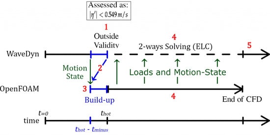
Finally, the proof of concept of the coupling is demonstrated. OpenFOAM starts when WaveDyn validity limit is estimated as attained, from WaveDyn RBM solution (i.e., position, velocity, and acceleration) and the imposed linear superposition for the wave-field (developed in [31]). Coupling demonstrates interest using the least steep event by reducing the computational effort by $26\%$ while maintaining accuracy to the level of CFD-only. A result considered to be applicable to the other events. A long irregular sea-state is used to indicate the coupling potential for long simulations that would be prohibitively expensive for CFD alone.

References

1. Ransley, E.; Jones, C.; Ma, Q.; Poulter, G.; Qian, L.; Tabor, G.; Yan, S.; Zang, J.; Greaves, D. Wave Structure Interaction Computation and Experiment Roadmap—Part 1: A Report on the 1st CCP-WSI Focus Group Workshop; PEARL Research Repository: Plymouth, UK, 2016. [Google Scholar] [CrossRef]
2. Westphalen, J.; Greaves, D.M.; Williams, C.K.; Taylor, P.H.; Causon, D.M.; Mingham, C.G.; Hu, Z.Z.; Stansby, P.K.; Rogers, B.D.; Omidvar, P. Extreme Wave Loading on Offshore Wave Energy Devices using CFD: A Hierarchical Team Approach. In Proceedings of the 8th European Wave and Tidal Energy Conference (EWTEC), Uppsala, Sweden, 7–10 September 2009. [Google Scholar]
3. Hu, Z.Z.; Greaves, D.; Raby, A. Numerical wave tank study of extreme waves and wave-structure interaction using OpenFoam®. Ocean Eng. 2016, 126, 329–342. [Google Scholar] [CrossRef] [Green Version]
4. Henry, A.; Schmitt, P.; Whittaker, T.; Rafiee, A.; Dias, F. The characteristics of wave impacts on an oscillating wave surge converter. In Proceedings of the 23rd International Offshore and Polar Engineering Conference (ISOPE), International Society of Offshore and Polar Engineers, Anchorage, Alaska, 30 June–5 July 2013. [Google Scholar]
5. Heilskov, N.F.; Petersen, O.; Fuchs, J. Structural Design of Wave Energy Converters—State-of-the-Art and Implementation of Design Tools for Floating Wave Energy Converters; Danish Hydraulic Institute: Hørsholm, Denmark, 2015. [Google Scholar]
6. O’Neill, L.; Fakas, E.; Cassidy, M. A methodology to simulate floating offshore operations using a design wave theory. J. Offshore Mech. Arct. Eng. 2006, 128, 304–313. [Google Scholar] [CrossRef]
7. Vyzikas, T.; Greaves, D.; Simmonds, D.; Maisondieu, C.; Smith, H.; Radford, L. Application of Numerical Models and Codes; Technical Report; Marine Energy in Far Peripheral and Island Communities (MERiFIC): Plymouth, UK, 2014. [Google Scholar]
8. International Electrotechnical Commission. Marine Energy—Wave, Tidal and Other Water Current Converters— Part 2: Design Requirements for Marine Energy Systems; IEC TS 62600-2:2016; IEC: Geneva, Switzerland, 2016. [Google Scholar]
9. Coe, R.; Yu, Y.H.; Van Rij, J. A survey of wec reliability, survival and design practices. Energies 2018, 11, 4. [Google Scholar] [CrossRef] [Green Version]
10. Ransley, E.; Yan, S.; Brown, S.; Mai, T.; Graham, D.; Ma, Q.; Musiedlak, P.; Engsig-Karup, E.; Eskilsson, C.; Li, Q.; et al. A blind comparative study of focused wave interactions with a fixed FPSO-like structure (CCP-WSI Blind Test Series 1). Int. J. Offshore Polar Eng. (IJOPE) 2019, 29, 113–127. [Google Scholar] [CrossRef] [Green Version]
11. Guanche, R. On the importance of calibration and validation procedures: Hybrid modeling. In Proceedings of the BCAM Workshop Hydrodynamics of Wave Energy Converter, Bilbao, Spain, 3–7 April 2017. [Google Scholar]
12. Windt, C.; Davidson, J.; Ringwood, J.V. High-fidelity numerical modelling of ocean wave energy systems: A review of computational fluid dynamics-based numerical wave tanks. Renew. Sustain. Energy Rev. 2018, 93, 610–630. [Google Scholar] [CrossRef] [Green Version]
13. Verbrugghe, T.; Domínguez, J.M.; Crespo, A.J.; Altomare, C.; Stratigaki, V.; Troch, P.; Kortenhaus, A. Coupling methodology for smoothed particle hydrodynamics modelling of non-linear wave-structure interactions. Coast. Eng. 2018, 138, 184–198. [Google Scholar] [CrossRef]
14. Dunbar, A.J.; Craven, B.A.; Paterson, E.G. Development and validation of a tightly coupled CFD/6-DOF solver for simulating floating offshore wind turbine platforms. Ocean Eng. 2015, 110, 98–105. [Google Scholar] [CrossRef] [Green Version]
15. Palm, J.; Eskilsson, C.; Paredes, G.M.; Bergdahl, L. Coupled mooring analysis for floating wave energy converters using CFD: Formulation and validation. Int. J. Mar. Energy 2016, 16, 83–99. [Google Scholar] [CrossRef] [Green Version]
16. De Lataillade, T.; Dimakopoulos, A.; Kees, C.; Johanning, L.; Ingram, D.; Tezdogan, T. CFD Modelling coupled with Floating Structures and Mooring Dynamics for Offshore Renewable Energy Devices using the Proteus Simulation Toolkit. In Proceedings of the 12th European Wave and Tidal Energy Conference (EWTEC), Cork, Ireland, 27 August–1 September 2017. [Google Scholar]
17. Proteus. A Python Toolkit for Computational Methods and Simulation. Source Code. 2019. Available online: https://proteustoolkit.org/index.html (accessed on 29 June 2020).
18. ProjectCHRONO. An Open Source Multi-Physics Simulation Engine. Source Code. 2019. Available online: https://projectchrono.org/ (accessed on 29 June 2020).
19. Li, Q.; Wang, J.; Yan, S.; Gong, J.; Ma, Q. A zonal hybrid approach coupling FNPT with OpenFOAM for modelling wave-structure interactions with action of current. Ocean Syst. Eng. 2018, 8, 381–407. [Google Scholar]
20. Hildebrandt, A.; Sriram, V.; Schlurmann, T. Simulation of focusing waves and local line forces due to wave impacts on a tripod structure. In Proceedings of the Twenty-third International Offshore and Polar Engineering Conference, International Society of Offshore and Polar Engineers, Anchorage, AK, USA, 30 June–5 July 2013; pp. 575–581. [Google Scholar]
21. Lachaume, C.; Biausser, B.; Grilli, S.; Fraunié, P.; Guignard, S. Modeling of Breaking and Post-breaking Waves on Slopes by Coupling of BEM and VOF Methods. In Proceedings of the Thirteenth International Offshore and Polar Engineering Conference, International Society of Offshore and Polar Engineers, Honolulu, HI, USA, 25–30 May 2003. [Google Scholar]
22. Paulsen, B.T.; Bredmose, H.; Bingham, H.B. An efficient domain decomposition strategy for wave loads on surface piercing circular cylinders. Coast. Eng. 2014, 86, 57–76. [Google Scholar] [CrossRef]
23. Biausser, B.; Fraunié, P.; Grilli, S.; Marcer, R. Numerical Analysis of the Internal Kinematics and Dynamics of Three-dimensional Breaking Waves on Slopes. Int. J. Offshore Polar Eng. 2004, 14, 247–256. [Google Scholar]
24. Sriram, V.; Ma, Q.; Schlurmann, T. A hybrid method for modelling two dimensional non-breaking and breaking waves. J. Comput. Phys. 2014, 272, 429–454. [Google Scholar] [CrossRef]
25. Kim, S.H.; Yamashiro, M.; Yoshida, A. A simple two-way coupling method of BEM and VOF model for random wave calculations. Coast. Eng. 2010, 57, 1018–1028. [Google Scholar] [CrossRef]
26. Yan, S.; Yamashiro, M.; Yoshida, A.; Ayukaw, K.; Irie, I. Development of a combined method of BEM and VOF for analyzing wave motion. Proc. Civ. Eng. Ocean 2003, 19, 83–88. [Google Scholar] [CrossRef]
27. Wang, J.; Ma, Q.; Yan, S. A hybrid model for simulating rogue waves in random seas on a large temporal and spatial scale. J. Comput. Phys. 2016, 313, 279–309. [Google Scholar] [CrossRef]
28. DNV-GL. WaveDyn—1.2; DNV-GL: Bristol, UK, 2018. [Google Scholar]
29. OpenFOAM.org. OpenFOAM—4.2; OpenFOAM.org: London, UK, 2018. [Google Scholar]
30. Musiedlak, P.H. Numerical Modelling of Responses of Offshore Wave Energy Converters in Extreme Wave. Ph.D. Thesis, Univeristy of Plymouth, Plymouth, UK, 2019. [Google Scholar]
31. Musiedlak, P.H.; Ransley, E.; Brown, S.; Greaves, D.; Child, B.; Hann, M.; Iglesias, G. Starting a wave structure interaction CFD simulation form an advance time: Hot-start. In Proceedings of the Sixth ECCM-ECFD Conference, Glasgow, UK, 11–15 June 2018; pp. 553–564. [Google Scholar]
32. Hann, M.; Greaves, D.; Raby, A.; Howey, B. Use of constrained focused waves to measure extreme loading of a taut moored floating wave energy converter. Ocean Eng. 2018, 148, 33–42. [Google Scholar] [CrossRef]
33. COAST Laboratory. Coastal, Ocean and Sediment Transport. 2019. Available online: https://www.plymouth.ac.uk/research/institutes/marine-institute/coast-laboratory (accessed on 29 June 2020).
34. Hann, M.; Greaves, D.; Raby, A. Snatch loading of a single taut moored floating wave energy converter due to focussed wave groups. Ocean Eng. 2015, 96, 258–271. [Google Scholar] [CrossRef] [Green Version]
35. Tromans, P.S.; Anaturk, A.R.; Hagemeijer, P. A new model for the kinematics of large ocean waves-application as a design wave. In Proceedings of the First International Offshore and Polar Engineering Conference (ISOPE), International Society of Offshore and Polar Engineers, Edinburgh, UK, 11–16 August 1991; pp. 64–71. [Google Scholar]
36. Walker, D.A.G.; Taylor, P.H.; Taylor, R.E. The shape of large surface waves on the open sea and the Draupner New Year wave. Appl. Ocean Res. 2004, 26, 73–83. [Google Scholar] [CrossRef]
37. Bateman, W.J.D.; Katsardi, V.; Swan, C. Extreme ocean waves. Part I. The practical application of fully nonlinear wave modelling. Appl. Ocean Res. 2012, 34, 209–224. [Google Scholar] [CrossRef]
38. Xu, L.; Barltrop, N.; Okan, B. Bow impact loading on FPSOs 1—Experimental investigation. Ocean Eng. 2008, 35, 1148–1157. [Google Scholar] [CrossRef]
39. Taylor, P.H.; Jonathan, P.; Harland, L.A. Time domain simulation of jack-up dynamics with the extremes of a Gaussian process. J. Vib. Acoust. 1997, 119, 624–628. [Google Scholar] [CrossRef]
40. Rafiee, A.; Wolgamot, H.; Draper, S.; Orszaghova, J.; Fiévez, J.; Sawyer, T. Identifying the design wave group for the extreme response of a point absorber wave energy converter. In Proceedings of the Asian Wave and Tidal Energy Conference (AWTEC), Singapore, 24–28 October 2016. [Google Scholar]
41. Halcrow. South West of England Regional Development Agency: Wave Hub Development and Design Phase Coastal Processes Study Report. 2006. Available online: https://www.wavehub.co.uk/downloads/EIA/wave-hub-final-design-report-june-2006.pdf (accessed on 29 June 2020).
42. Hunt-Raby, A.C.; Borthwick, A.G.; Stansby, P.K.; Taylor, P.H. Experimental measurement of focused wave group and solitary wave overtopping. J. Hydraul. Res. 2011, 49, 450–464. [Google Scholar] [CrossRef] [Green Version]
43. Ning, D.; Zang, J.; Liu, S.; Taylor, R.E.; Teng, B.; Taylor, P. Free-surface evolution and wave kinematics for nonlinear uni-directional focused wave groups. Ocean Eng. 2009, 36, 1226–1243. [Google Scholar] [CrossRef]
44. Hann, M.; Greaves, D.; Raby, A.C. A new set of focused wave linear combinations to extract non-linear wave harmonics. In Proceedings of the 29th International Workshop for Water Waves and Floating Bodies, Osaka, Japan, 30 March–2 April 2014; pp. 61–64. [Google Scholar]
45. Jasak, H. Error Analysis and Estimation for the Finite Volume Method with Applications to Fluid Flows. Ph.D. Thesis, Imperial College London (University of London), London, UK, 1996. [Google Scholar]
46. Sumer, B.M. Hydrodynamics around Cylindrical Strucures; World Scientific: Singapore, 2006; Volume 26. [Google Scholar]
47. Ransley, E.J. Survivability of Wave Energy Converter and Mooring Coupled System Using CFD. Ph.D. Thesis, Plymouth University, Plymouth, UK, 2015. [Google Scholar]
48. Vyzikas, T.; Ransley, E.; Hann, M.; Magagna, D.; Greaves, D.; Simmonds, D.; Magar, V.; Conley, D. Integrated numerical modelling system for extreme wave events at the wave hub site. In Proceedings of the ICE Conference on Coasts, Marine Structures and Breakwaters, Edinburgh, UK, 18–20 September 2013. [Google Scholar]
49. Jacobsen, N.G.; Fuhrman, D.R.; Fredsøe, J. A wave generation toolbox for the open-source CFD library: OpenFoam®. Int. J. Numer. Methods Fluids 2012, 70, 1073–1088. [Google Scholar] [CrossRef]
50. Anderson, J.J.D. Computational Fluid Dynamics: The Basics with Applications; McGraw-Hill International Editions: New York, NY, USA, 1995. [Google Scholar]
51. Ransley, E.; Greaves, D.; Raby, A.; Simmonds, D.; Hann, M. Survivability of wave energy converters using CFD. Renew. Energy 2017, 109, 235–247. [Google Scholar] [CrossRef] [Green Version]
52. Greaves, D.M.; Borthwick, A. Hierarchical tree-based finite element mesh generation. Int. J. Numer. Methods Eng. 1999, 45, 447–471. [Google Scholar] [CrossRef]
53. Cummins, W.E. The Impulse Response Function and Ship Motions; Technical Report; (No. DTMB-1661); David Taylor Model Basin: Washington, DC, USA, 1962. [Google Scholar]
54. Newman, J.N.; Sclavounos, P.D. The computation of wave loads on large offshore structures. In Proceedings of the 5th International Conference on the Behaviour of Offshore Structures (BOSS 88’), Trondheim, Norway, 7–10 July 1988; Volume 2, pp. 605–622. [Google Scholar]
55. Babarit, A.; Delhommeau, G. Theoretical and numerical aspects of the open source BEM solver NEMOH. In Proceedings of the 11th European Wave and Tidal Energy Conference (EWTEC2015), Nantes, France, 6–11 September 2015. [Google Scholar]
56. Galton, F. Regression towards mediocrity in hereditary stature. J. Anthropol. Inst. G. B. Irel. 1886, 15, 246–263. [Google Scholar] [CrossRef]
Figure 2. Time-splitting strategy as function of time.
Energies 13 03431 g002
Figure 3. Extreme loading of marine energy devices due to waves, current, flotsam and mammal impacts (X-MED) model [32].
Energies 13 03431 g003
Figure 4. S T surface-elevations time-series.
Energies 13 03431 g004
Figure 5. Surface elevations time-series for four of the twelve S T 1 - f o c u s e d events.
Energies 13 03431 g005
Figure 6. The 20 × 1.5 × 4 m 3D-NWT developed for extreme WSI [30].
Energies 13 03431 g006
Figure 7. Surface-elevation and motion responses time-series of the X-MED buoy under S T events.
Energies 13 03431 g007
Figure 8. Correlation (R) between each numerical model and experiment.
Energies 13 03431 g008
Figure 9. Evaluation of the lower angle in the step of the NRMS time-series.
Energies 13 03431 g009
Figure 10. Identification of wave-parameters at deviation point for S T 1 . | is the deviation point, | is the second largest peak (i.e., a non-deviating point).
Energies 13 03431 g010
Figure 11. Evolution of | η | identified at deviation and non-deviating points for all events.
Energies 13 03431 g011
Figure 12. Estimation of the deviation point using the WaveDyn’s validity limit (| identifies | η | < 0.549 m / s ) applied to an irregular extreme sea-state.
Energies 13 03431 g012
Figure 13. CFD motion responses time-series when conventionally started and when hot-started at focus (Hot-started with t m i n u s = 4 s and 5 time-steps for RBM build-up).
Energies 13 03431 g013
Figure 14. Heave decay responses demonstrating coupling at hot-start time t h o t = 0.1 s ( t m i n u s = 0 ).
Energies 13 03431 g014
Figure 15. Comparison of numerical models motion responses prediction time-series using S T 1 case. | indicate hot-start time ( t h o t ) and when coupling starts ( t h o t t m i n u s ).
Energies 13 03431 g015
Figure 16. Comparison of motion response time-series between experiment and numerical models prediction where the hybrid model is triggered by WaveDyn’s validity limit. | indicate hot-start time ( t h o t ) and when coupling starts ( t h o t t m i n u s ).
Energies 13 03431 g016