Article

Virtual Simulation of Electric Bus Fleets for City Bus Transport Electrification Planning

Faculty of Mechanical Engineering and Naval Architecture, University of Zagreb, 10002 Zagreb, Croatia
*
Author to whom correspondence should be addressed.
Energies 2020, 13(13), 3410; https://doi.org/10.3390/en13133410
Submission received: 20 May 2020 / Revised: 24 June 2020 / Accepted: 26 June 2020 / Published: 2 July 2020

Abstract

:
City bus transport electrification has a strong potential of improving city air quality, reducing noise pollution and increasing passenger satisfaction. Since the city bus operation is rather deterministic and intermittent, the driving range- and charging-related concerns may be effectively overcome by means of fast charging at end stations and/or slow charging in depot. In order to support decision making processes, a simulation tool for planning of city bus transport electrification has been developed and it is presented in this paper. The tool is designed to use real/recorded driving cycles and techno-economic data, in order to calculate the optimal type and number of e-buses and chargers, and predict the total cost of ownership including investment and exploitation cost. The paper focuses on computationally efficient e-bus fleet simulation including powertrain control and charging management aspects, which is illustrated through main results of a pilot study of bus transport electrification planning for the city of Dubrovnik.

Graphical Abstract

1. Introduction

Due to environmental concerns, there is a strong tendency of electrifying road transport systems by means of introducing different types of electric vehicles [1]. Apart from reducing pollutant and CO2 emissions, electric vehicles (EV) are characterised by substantially reduced noise pollution, lower operating cost (including energy and maintenance cost) and generally better driving characteristics. On the other hand, higher investment cost, slow battery charging and limited driving range inhibit their faster proliferation [2]. This is why the transition to fully electric vehicles (FEV or BEV) is characterised by application of hybrid electric vehicles (HEV) and plug-in hybrid electric vehicles (PHEV) [3].
City bus transport is a natural candidate for electrification, aiming at improvement in city air quality and reduction of noise. Since the city bus routes are known in advance and the operation is intermittent, the range- and charging-related issues are of lesser significance than with passenger cars. These issues can be tackled by the following two basic approaches [4]: (i) the buses are equipped with large enough battery packs to sustain half a day or even full day of operation, and the buses are efficiently recharged by using slow charging (typically overnight); and (ii) the battery size is minimised and superfast charging is employed at bus stops (typically end stations). Therefore, it is generally of interest to find optimal locations of charging stations, as considered in [5,6,7,8,9,10,11] with a focus on passenger cars and urban areas.
In [12], e-buses and corresponding charging systems are analysed from the total cost perspective by using data related to route specifications, timetables and other local conditions. Additionally, the authors have developed a user-friendly tool which enables the user to investigate and quantify trade-offs between EV battery size, charging infrastructure cost and vehicle fleet operational costs. However, all routes are modelled as straight lines between the bus stops and elevation is collected only at stops, thus hiding some relevant topographical features along the routes and affecting the analysis accuracy. In [13], a stochastic integer program was developed to jointly optimise charging station locations and bus fleet size, while considering stochastic bus charging demand and time-of-use electricity tariffs for the case of real-world network in Melbourne. However, this study does not consider charging scheduling for individual buses. The aforementioned city bus transport optimisation study [4] relies on an artificial urban bus driving cycle when conducting bus fleet simulations, thus neglecting influential effects of city traffic congestion, road slopes, often stops and so on. The authors of [14] indicated that lowering the fuel cost for electric buses can balance the high investment costs related to building charging infrastructure, while additionally achieving a significant reduction in pollutant emissions. To that extent, detailed techno-economic analyses comparing the total cost of ownership (TCO) of conventional and EV fleets should be conducted [15].
To the best of the authors’ knowledge, studies dealing with extensive virtual simulations of different e-bus-type fleets based on real-life driving cycles and concerning spatially-distributed charging management and related TCO analyses have not been considered in the literature thus far. To fill the gap, a unique simulation tool for planning of city bus transport electrification, which contains all of the above functionalities, has been developed, which is described in this paper, including its application to a pilot study for the City of Dubrovnik. The tool consists of four modules aimed at (i) post-processing and statistical analysis of a large set of recorded driving cycles, (ii) simulation of conventional (CONV) and different types of e-buses (HEV, PHEV and BEV), (iii) virtual simulation of e-bus fleets over recorded driving cycles including user-defined setting of charging station locations and charging management itself and (iv) techno-economic analyses. The main contributions of the paper include: (i) creating a unique and flexible/transferable simulation tool resulting in realistic, data-driven transport electrification analyses; (ii) building a static map-based form of HEV/PHEV-type bus model including its control strategy, which drastically boost computational efficiency of large-scale fleet simulations; (iii) performing a detailed techno-economic analysis based on realistic virtual bus fleet simulation and actual technical data provided by city bus transport companies.
The paper is organised as follows. Section 2 describes the methodology of recording driving cycle data and overviews the structure of developed simulation tool. Section 3 outlines the Data Post-Processing Module (DPPM) and presents corresponding results of conventional city-bus transport system characterisation. Section 4 deals with E-Bus Simulation Module (EBSM) and discusses belonging simulation results for the four considered types of city buses. Section 5 describes the Charging Optimisation Module (COM) and overviews the results related to obtaining near-optimal charging infrastructure configuration for the cases of PHEV- and BEV-type bus fleets. The Techno-Economic Analysis Module (TEAM) is briefly described in Section 6, and the corresponding TCO results are discussed for various e-bus fleet scenarios. Concluding remarks are given in Section 7.

2. Pilot Data and Simulation Tool Structure

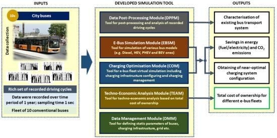
2.1. Recording of Driving Cycle Data

The driving cycle data have been collected on a sub-fleet of 10 MAN Lyon’s City NL323 buses operating in the city of Dubrovnik. They are considered a good representative of the overall fleet, as they cover all major bus routes (Figure 1) and represent around 1/3 of regularly used city buses. The driving data recording was performed by utilising a commercial GPS/GPRS vehicle tracking device installed in the selected buses for the purpose of this study. The data, collected from a built-in GPS device and vehicle CAN bus, are summarised in Table 1. Recording was conducted continuously for a period of five months, and the data sampling time was 1 second.

2.2. Organisational Structure of Simulation Tool

Figure 2 illustrates the structure of the developed tool, including the connections between the main modules. The tool is driven by recorded driving cycle data, and as the main output, it delivers the TCO over the projected fleet operational period (12 years, herein). The DPPM transforms the recorded driving data into individual driving cycles, and it also calculates various statistical features characterising the conventional city bus transport behaviours. The EBSM provides computer simulations of different types of city buses (CONV, HEV, PHEV, BEV) over the driving cycles extracted by the DPPM. The module outputs include the individual bus energy consumption (fuel and/or electricity) and various features of powertrain response (e.g., engine/e-motor operating points, gear ratio trajectories, etc.). The COM utilises the outputs of DPPM and EBSM to simulate the overall city bus fleet over the recorded driving cycles and optimise the PHEV- and BEV-type bus charging configuration and management. This module provides the number, location and type of chargers, the bus battery capacity and the number of reserve buses in the BEV case, which are required to fulfil the driving routes with sufficient battery charge. The COM also outputs the total fuel and/or electricity consumption over the considered period of operation. The TEAM uses the output data from the COM module, as well as the data on bus transport investment and exploitation/maintenance cost, in order to calculate the TCO.
The simulation tool is written in Python object-oriented programming language, with computationally demanded routines coded in C language. The Python language has been selected because it is available in open-source domain, it supports multiple platforms, has a vast number of available libraries, and is dynamically typed language (i.e., does not require declaring of data type of a variable) convenient for rapid prototyping. The simulation tool is designed in a user-friendly way (based on a graphical user interface (GUI) including windows, tabs, I/O data interfaces, etc.) and has in mind the transferability to other cities using a common/shared database. The database serves as a main storage for recorded driving cycle data, and plays the role of an intermediary between the main tool modules. In addition, the simulation tool includes the Data Management Module (DMM), which provides greater flexibility and adaptability to different cities’ transport system configurations. DMM enables the user to define all static data (system parameters) required by the simulation tool, e.g., those related to vehicle model parameters, end-station and depot locations, charging station parameters and techno-economic data.

3. Data Post-Processing Module (DPPM)

3.1. General Description

According to the DPPM flowchart shown in Figure 3, the recorded driving data are first processed and stored in a database. Next, the driving cycles are extracted by using the DMM-based data related to geographical coordinates of end stations and depot (Section 3.2). At the same time, the fleet statistics are calculated for the entire fleet and individual buses (Section 3.3). Finally, the module outputs including driving cycles and statistical features can be plotted in different formats, and they are saved into the database.

3.2. Extraction of Driving Cycles

A single driving cycle is defined by the velocity vs. time and road slope vs. travelled distance profiles between two consecutive end stations, including depot (see Figure 1). The corresponding time profiles of cumulative fuel consumption are also extracted.
The driving cycle segmentation process resulted in a total of 122,727 extracted driving cycles. An example of recorded driving cycle is shown in Figure 4. Note that the vehicle velocity is directly measured, while the road grade is reconstructed from the rate of change of altitude when expressed with respect to the travelled distance. In order to reduce the noise in the reconstructed road slope profile, the altitude signal is pre-filtered by a low-pass double-sided Butterworth filter [16].

3.3. Calculation of Vehicle Fleet Statistics

A rich set of statistically significant driving features is calculated for the purpose of actual/conventional city-bus transport system characterisation and in support of transport electrification (e.g., locating charging stations, Section 5). The features related to individual buses, all given per-day-basis, include: the total fuel consumption and distance travelled; average fuel consumption in L/100 km; the total time the bus is dwelling at depot, individual end stations or any other locations (typically bus stops); total driving time; mean velocity; number of bus stops per kilometre; number of bus visits to depot and end stations. The results are stored in a two-dimensional (2D) matrix (one per bus), whose rows and columns represent individual days and the statistical features, respectively.
Once the individual statistics are stored, they are further used to calculate the same features for the entire fleet on the basis of individual day, week, month or year. The results can be presented in different ways, e.g., instead of individual dwelling times, one can get the information about percentage share of time the buses or entire fleet are resting at depot, end stations and other locations (see Figure 5). Specific fleet features requiring denser sampling (30 min, herein) are also calculated. An example of the daily average fleet velocity profile is shown in Figure 6. Other features related to entire fleet include: average number of buses being parked at depot on 24-hour time basis (Figure 6), clusters of buses parking durations in relation to geographical coordinates, count of transitions between individual end stations/depot, etc.
Figure 6 indicates that the average bus velocity when operating is around 30 km/h and it is higher in early morning and night hours, as well as over weekends. The low-velocity gap between 2 a.m. and 5 a.m. corresponds to the interval when most of the buses are parked in the depot. The buses rarely visit the depot in other time intervals, particularly over the work days (when the average number of buses is lower than 1).
Figure 5 confirms that the share of total time of buses being parked in the depot is relatively small (approx. 30%) and comparable to the share of end-station parking time (approx. 25%). The rest of the time the buses spend in driving (40%), while only for a small portion of time (approx. 5%), they rest elsewhere, typically at bus stops.
Figure 7a indicates that there are significant differences in bus resting time at different end stations. The average resting durations for most pronounced end stations are between 10 and 20 min, thus making them good candidates for installation of fast chargers. When selecting the best candidates, a charging station utilisation factor should also be considered (Figure 7b). The final end stations targeted for electrification are then obtained by taking the cross-section of these two criteria (end stations underlined in red in Figure 7).

4. E-Bus Simulation Module (EBSM)

4.1. General Description

As illustrated in flowchart in Figure 8, the EBSM simulates different types of city buses (CONV, HEV, PHEV and BEV) over the recorded driving cycles extracted by the DPPM (Section 3). The simulation first involves loading of vehicle-related parameters from the database, which need to be previously defined in the DMM. Next, the vehicle is simulated over the selected driving cycles by using the numerically-efficient backward-looking model (Section 4.2). Note that the vehicle model includes a control strategy that manages the gear ratio in the CONV and BEV cases, and the internal combustion engine (ICE) torque in the HEV and PHEV cases (Section 4.3). The emphasis has been on transforming the previously developed control strategy [17,18] to a form of off-line optimised maps, instead of using an on-line optimisation algorithm. The EBSM outputs time responses of key powertrain variables, such as cumulative fuel and electricity consumption, CO2 emissions and transmission gear ratio.

4.2. Vehicle Modelling

4.2.1. Considered City Buses

The MAN Lion’s City buses with the length of 12 m and the capacity of up to 126 passengers are represented in virtual simulation by the Volvo 7900 bus model. The Volvo 7900 platform was chosen because it includes all three e-bus variants considered (HEV, PHEV and BEV; Table 2).
Volvo e-buses use lithium iron phosphate (LFP) battery due to its high specific power required for propulsion and fast charging. The battery packs of Volvo 7900 HEV, PHEV and BEV bus variants have energy capacities of 4.8 kWh, 19 kWh and 76 kWh, respectively (Table 2).

4.2.2. Modelling

In the backward-looking models, the powertrain variables are calculated in the direction from the wheels towards the engine and/or e-motor, starting from the wheel speed and torque being defined by the driving cycles [20]. In order to boost the computational efficiency, the powertrain dynamics is neglected, except for the battery state-of-charge (SoC) dynamics that are represented by a first-order model.
The considered parallel configuration of a HEV/PHEV-type bus is illustrated in Figure 9a [17]. The battery is represented by the equivalent battery circuit model shown in Figure 9b, which is described by the following state equation [20,21]:
S o ˙ C ( t ) = I b a t t ( t ) Q max = U o c 2 ( S o C ) 4 R ( S o C ) P b a t t ( t ) U o c ( S o C ) 2 Q m a x R ( S o C )   ,
where Uoc is the open-circuit voltage, R is the internal resistance, Ibatt is the battery current, Qmax is the maximal battery charge capacity and the SoC is defined as SoC = Q/Qmax, with Q denoting the actual charge.
The model input Pbatt represents the battery output power defined as:
P b a t t = η M G k · τ M G · ω M G   ,
where τMG and ωMG are the motor/generator (M/G) torque and speed, respectively, ηMG is the M/G machine efficiency (represented by ηMG(ωMG,τMG) map; see Figure 10c and [17]) and the coefficient k is equal to 1 or −1 depending on whether the M/G machine operates as a generator or motor, respectively. The M/G machine speed and torque are given by the following kinematic equations:
ω M G = i o h ω w = i o h v v r w   ,
τ M G = τ w η t r ( τ w ) + P 0 ( ω w ) ω w i o h τ e   ,
where vv is the vehicle velocity, rw is the tire effective radius, h and i0 are the transmission and final drive ratios, respectively, τw and ww are the total wheels torque and speed, respectively, ηtr(τw) and P0(ωw) are drivetrain efficiency and idle power loss maps [17] and τe is the engine torque considered as a control variable (in addition to h). The wheel torque is determined according to vehicle longitudinal dynamics equation covering the vehicle acceleration torque and aerodynamic, road grade and rolling resistances [20].
The fuel consumption at the driving cycle end time tf is determined as:
V f = 1 ρ f u e l 0 t f m ˙ f d t = 1 ρ f u e l 0 t f ( A e k ( τ e , ω e ) τ e ω e 3.6 · 10 6 ) d t   ,
where Aek is the engine specific fuel consumption given by the map shown in Figure 11, ρfuel is the diesel fuel density (ρfuel = 845 g/L) and ωe equals ωMG or 0 when the engine is switched on or off, respectively. Note that the integral Equation (5) is realised by using the Euler integration method with the common sample time of the backward model equal to 1 s.
In the case of a conventional (CONV) bus, the battery and M/G machine are omitted from the functional scheme in Figure 9, while the AMT is replaced by a torque converter AT. The torque converter is represented by a backward-looking map ωι (ωt,τt) derived offline from the well-known static torque converter model (see [22] and references therein) and the map τ i = τ t / Rτ (ω t/ω i), where the subscripts i and t denote impeller/engine and turbine/transmission input variables, and Rτ (.) is the static model torque ratio map. For the BEV-type bus, the engine is omitted and a two-speed AMT is used.
Vehicle auxiliary devices (HVAC system, servo steering, air compressor, engine cooling fan and alternator) are modelled based on the nominal power of each device and a binary power-modulating signal, whose duty cycle is made dependent on the driving and atmospheric conditions (urban driving conditions and ambient temperature dependence are assumed) [23].

4.3. Control Strategy

In the BEV case, the aim of control strategy is to find an optimal gear ratio h* in each sampling instant, which minimises the battery discharging power and maximises the battery recharging/regenerative power:
h * = argmin h { η b a t t k P b a t t ( P d , ω w , h ) , for   P b a t t < 0   ( charging ) η b a t t k P b a t t ( P d , ω w , h ) , for   P b a t t 0   ( discharging ) ,
where ηbatt is the battery efficiency and Pd is the transmission input power demand calculated from vv and τw as shown in Figure 12. The optimal gear ratio h* is calculated offline and mapped as h* (Pd, ωw). The SoC dependence of Pbatt has a minor effect on h* and is neglected in Equation (6), and further on.
Similarly, in the CONV case, the control strategy finds an optimal gear ratio h* that minimises the fuel mass flow f:
h * = arg min h m ˙ f ( P d , ω w , h )   .
The off-line obtained optimal solutions are mapped as h*(Pd, ωw).
The HEV and PHEV control strategy determines the transmission gear ratio h and the engine torque τe based on combining a rule-based (RB) controller and an equivalent consumption minimisation strategy (ECMS) [17,24]. The original RB+ECMS strategy is modified here to allow for computationally-efficient map-based realization, which is shown in Figure 12. A proportional-like battery SoC controller commands the battery recharging power—Pbatt, which is added to the transmission input power demand Pd to obtain the engine power demand P*e. The demanded engine power P*e is compared with engine on and off thresholds Pon and Poff < Pon, respectively, in order to determine the engine on/off state ENst. The engine is exceptionally kept switched on in the case P*e < Poff when the speed-dependent M/G machine power limit is not high enough to satisfy the driver power demand Pd in the fully electric driving mode. If the engine is switched on, the signal P*e is fed to the ECMS to find the optimal values of h and τe. Otherwise, the electric driving mode is activated and the gear ratio is determined according to Equation (6).
In the original RB+ECMS strategy [17], the equivalent fuel consumption eq(Pe, Pd, ωw, h, SoC) is minimised instantaneously and on-line with respect to both control variables h and τe. In the simplified map-based RB+ECMS version considered here, the equivalent fuel consumption is minimised in two stages. In the first stage, the ECMS is applied to discrete operating points along the constant power curve P*e (denoted in Figure 11 by blue circles) to determine the optimal gear ratio:
h * = arg min h   m ˙ e q ( P e * ,   P d , ω w , h )   ,
where eq is the equivalent fuel consumption rate containing the actual fuel consumption rate f and a battery power-equivalent fuel rate (see [17,24] for details). The off-line obtained optimal solutions are stored in a three-dimensional (3D) map h*(P*e, Pd, ωw) representing the RB+1D-ECMS control map. In the second stage, the ECMS is applied along the engine torque axis (see green arrows in Figure 11):
τ e , 2 D * = argmin τ e   m ˙ e q ( P d , ω e , τ e )   .
The off-line optimisation results are stored in a 2D map τ*e,2D(Pd, ωe) representing the 2D-ECMS control map. Finally, the engine torque obtained by the RB+1D-ECMS (as τ*e,RB = P*e/(h*ioωw)) and the one obtained by the 2D-ECMS are combined/blended on-line using the SoC control error (eSoC)-dependent weighting factor W(eSoC) [17,24]:
τ e * = τ e , R B * W ( e S o C ) + τ e , 2 D * ( 1 W ( e S o C ) )   ,
where W(.) is an SoC control error-dependent weighting function illustrated in Figure 12. For small SoC control errors, the 2D-ECMS is dominant, while for large SoC control errors, the RB+1D-ECMS is preferred to satisfy the engine power demand P*e (and, thus, the battery power demand P*batt).
Finally, gear shift delay logic is implemented to prevent frequent gear switching [17]. The goal is to prevent gear shift occurrence in kth time step, i.e., rather use the gear ratio from the previous (k−1)th step, hk−1, if the time elapsed since the last gear shift tsh is lower than an arbitrarily set shift delay threshold tth and if hk−1 gives feasible set uk of engine and M/G machine operating points in the kth step (denoted by Π):
h k * = { h k 1 * ,   for   t s h < t t h   and   u k ( P e * , P d , k , ω w , k , h k 1 * ) Π h * ( P e , k * , P d , k , ω w , k ) ,   otherwise  
The same gear shifting delay logic is applied in the CONV and BEV cases. The shift delay threshold is set here to tth = 2 s.
The above described simplified, map-based control strategy has been found to result in a negligible model response deviation when compared to the use of original strategy, which was proven to be close to the dynamic programming-based global optimum [17]. On the other hand, the execution time is reduced by around 200 times. The achieved execution time, expressed as the amount of microseconds needed to simulate one second of real time (for a workstation having 16 GB RAM and Intel® Xeon® Processor E5-1620 v3 @ 3.50GHz) falls in the range from 50 to 87 μs/s depending on vehicle type. This results in approximate yearly 10-bus fleet simulation time ranging from approximately 4.5 h to 7.5 h, which is deemed acceptable for such a large-scale fleet simulation. Note that the execution time could further be reduced by using parallel computing.
The PHEV can operate in two characteristic modes [20]: (i) charge depleting (CD) followed by charge sustaining (CS), where the former involves the engine only when absolutely needed and the latter correspond to hybrid operation at the target SoC of 30%; (ii) blended mode where engine is regularly used all over the driving cycle for additional energy savings. For the sake of simplicity, the CD/CS mode is considered in this paper.

4.4. Simulation Results

The results related to relative fuel and/or electricity consumptions for different city bus types are given in Table 3 for the full recording period. The relative difference between the simulated (Sim) and recorded (Rec) fuel consumptions for the CONV bus is equal to only 1.4%. Therefore, the CONV simulation model used as a basis for e-bus modelling can be considered accurate. Note that although the real and simulated buses are different (MAN Lion City and Volvo 7900), the validation is considered fair, as the two buses are rather comparable in terms of size, mass, engine power, number of passengers and other similar factors.
The simulated electricity consumptions of PHEV- and BEV-type buses are close to recorded ones documented in the ZeEUS project report [25] for Volvo 7900 bus series (Table 3). In the PHEV case, the simulated fuel consumption is by 30% higher than the ZeEUS recorded one, but this discrepancy is compensated for by 26% higher recorded electricity consumption when compared to the simulated one. In the BEV case, the relative difference in electricity consumption equals 6%. The simulated HEV fuel consumption is reduced by 50% when compared to CONV simulation results, while the manufacturer states the fuel consumption reduction from 39% to 45% reported by operators [19]. The observed, relatively modest discrepancies in fuel/electricity consumption may be related to difference in considered bus weights (passenger weight is fixed to 1250 kg), road slope and traffic congestion conditions, as well as regenerative braking capacity (set to the maximum amount of 100% in simulation).
Figure 10 shows the PHEV-case simulation results for the recorded driving cycle shown in Figure 4 repeated 15 times and the initial battery SoC equal to 90%. When the CD mode is active, the engine is used only when needed and the cumulative fuel consumption is often constant (a stepwise-like response, Figure 10a). After entering the CS mode, the engine is more active to sustain the battery SoC (Figure 10b). The control strategy deploys the operating points of engine (when switched on) and M/G machine in the high efficiency areas of corresponding maps (Figure 10c–d), thus minimising the energy consumption.

5. Charging Optimisation Module (COM)

5.1. General Description

A generic framework for virtual simulation of an e-bus fleet over the recorded driving cycles is represented by the flowchart shown in Figure 13. The model of city bus of any type (Section 4) is initialised based on the data stored in DMM and virtually run over the recorded driving cycles for the specified period of time, thus resulting in fuel and/or electricity consumption output data. In the case of a PHEV- or BEV-type bus the user needs to specify locations and types of charging stations, the nominal vehicle battery capacity and grid power constraints to execute the simulation. The simulation is repeatedly run for a peak day or peak week for different charging infrastructure and battery capacity specifications, in order to find a nearly-optimal configuration, which would be finally re-run for a given, longer period of time to calculate the fuel/electricity consumption and charging station utilisation statistics. In the case of BEV-type bus, the COM automatically adds reserve bus(es) if needed, and calculate their final number and related statistics. The bus intervening algorithm monitors each BEV’s battery SoC, and when it drops below a predefined minimum value (0.3, herein), the immediate replacement with reserve e-bus is conducted. At the same time, it is taken into account that the depleted bus needs some constant time to reach the nearest charging station, where it is to be charged (as any other bus), and once it is fully charged, it will be waiting for the next replacement/intervention.

5.2. Charging Management Algorithm

Charging management is described by the flowchart shown in Figure 14. First, it is checked if a PHEV- or BEV-type bus has arrived to an end station/depot and if that station has a charger installed. If the charger is not occupied or if the bus has a lower battery SoC of any of the buses already being charged, the bus is put on charge; otherwise, it remains in the charging queue. Note that each station can be set to have an arbitrary number of chargers, as described with Figure 13.
The charging process is managed by taking into account the requirements on satisfying the departure schedule, minimising battery power loss and respecting the grid power constraints. According to [26,27], the battery energy loss is minimised by demanding a linear change of SoC all over the remaining charging interval Δ T c h = t f t k . Therefore, the SoC rate is updated in each sampling instant k according to:
d S o C d t = S o C f S o C k t f t k   ,
where SoCk is the current SoC and SoCf is the target SoC at departure. Inserting Equation (12) into the battery state Equation (1) yields the charging power Pbatt < 0 to be applied in the kth sampling instant:
P b a t t = U O C 2 ( S o C k ) [ 2 Q m a x R i n t ( S o C k ) S o C f S o C k t f t k + U O C ( S o C k ) ] 2 4 R i n t ( S o C k )   .
If the charging power −Pbatt calculated from Equation (13) is greater/less than the maximum/minimum allowable power (defined by the charger selected), the charging power is limited to the maximum/minimum power, respectively. Note that Δ T c h = t f t k is saturated in Equation (13) to its lower limit of 30 s to avoid division by zero.
Once the charging power profile is obtained for each sampling step k and for ith vehicle from the total number of Nv vehicles connected to chargers at the same grid sections (e.g., depot), it is checked if the total charging power is greater than the maximum grid power P g r i d , m a x . If this applies, the charging power is scaled down to satisfy the grid power constraint:
P b a t t , k , i , c o r r = P g r i d ,   m a x i = 1 N v P b a t t , k , i P b a t t , k , i , if   i = 1 N v P b a t t , k , i > P g r i d ,   m a x   .

5.3. Obtaining of Near-Optimal Charging System Configurations

According to the city bus transport characterisation results from Figure 7, there is a number of end stations with relatively long bus resting durations and potentially high utilization of charger units. Additionally, the end station resting time share approaches that of depot (Figure 5), and there are no other emphasised stop locations. Therefore, fast charging stations and belonging transformer substations can be installed at end stations to provide bus recharging, while otherwise the available power can be utilised to supply city e-mobility hubs built around the end stations. High-power off-board chargers with built-in pantograph are considered (150 or 300 kW, see Table 2) [19]. In addition, the slow-to-modestly fast plug-in charging solutions can be considered for a depot, where the charging time can be long in night (Figure 6).

5.3.1. PHEV Fleet Case

Figure 15 shows the PHEV fleet simulation results for different number of end stations equipped with a single fast charger per station (150 kW) and a five work day period. Charging in depot was not considered because the small-capacity PHEV battery (Table 2) can quickly be recharged at the end stations, where the buses rest for a relatively long time (Figure 6 and Figure 7). The results shown in Figure 15 point out that the fuel consumption saving converges to −41% as the number of end station charging spots approaches six. Of course, as the fuel consumption reduces, the electricity consumption grows, but the overall energy cost is reduced by 17% due to cheaper electricity. By conducting PHEV fleet simulations over the five-month period, it has been found that the optimal number of charging stations should be incremented to seven.

5.3.2. Case of BEV Fleet

The BEV fleet simulation results are shown in Table 4. The full five-month period is considered to cover a larger number of “critical” days when reserve buses may be needed. Only scenarios with the number of end-station charging spots being in the vicinity of the optimal one found for the PHEV fleet is examined (around six stations plus depot, each considering a single fast charger). The maximum charging power is set to the levels of 150 kW or 300 kW. Finally, various battery capacities are considered (76, 150 and 250 kWh, as the capacities available for the considered bus [19]).
The results shown in Table 4 point out that by increasing the number of charging stations, the percentage of total electricity consumed by reserve buses drops from 9.2% (case BEV 1) to 1.8% (case BEV 2). Likewise, the number of bus swaps (concerning reserve bus) drops from 558 in 106 (out of 152) days (BEV 1) to 94 in 54 days (BEV 2). Figure 16 indicates that in the case BEV 2 notable bus swaps occurs only in several days, which are characterised by peak traffic load (typically due to specific needs such as moving tourists from cruising ships to the old city). Similar trends apply to the case of increasing the battery capacity from 76 kWh to 150 kWh and further to 250 kWh (cases BEV 4 and BEV 5, respectively), where the reserve buses are marginally needed in the former case, and not needed in the latter case.
Based on the above results, the case BEV 5 might be considered as optimal. However, since increasing of the battery capacity of each bus in a fleet is rather expensive and the need for reserve buses in case BEV 2 is minor (only 1.8%), the case BEV 2 has been adopted as an optimal for final simulations discussed in Section 5.4.

5.4. Comparative Energy Consumption Results

Table 5 gives the energy consumption simulation results for the PHEV and BEV fleets configured in the previous two sections, as well as HEV and CONV fleets, all simulated over the full recording period. The HEV fleet can reduce the fuel consumption by around 50% compared to CONV fleet, owing to regenerative braking, switching the engine off in low speed conditions and placing the engine operating points in the high-efficiency region (Section 4; see also Table 3). Using the PHEV buses provides additional fuel savings, i.e., the fuel consumption reduction compared to CONV case is around 70%. This is due to the use of electricity coming from grid by means of fast charging at end stations. The PHEV fleet electricity consumption equals almost 50% of what is consumed by BEV fleet, which is owing to a relatively low portion of operation in the CS mode (25.5%).
The COM also calculates the well-to-wheel CO2 emissions taking into account the data on CO2 emissions of power plants, as used in [28] for the cases considering coal, natural gas and renewable energy production. The HEV vs. CONV fleet CO2 emissions reduction is around 50%, while in the cases of PHEV and BEV fleets, the reduction is from 30% to 65% and from 30% to 93%, respectively, where the lower and higher margins correspond to coal and renewable energy production scenarios.

6. Techno-Economic Analysis Module (TEAM)

6.1. General Description and TCO Model

According to Figure 2, the TEAM uses the simulation data outputted by the COM, as well as the fleet loan payment, insurance, registration, maintenance and similar costs provided by DMM, in order to calculate the fleet TCO (Figure 17). The TCO corresponds to what is in financial terminology called Net Present Value (NPV) of an investment, which is an index that valorises the investment while considering the time value of money. Rates at which the money value decreases or increases over time are in this case modelled by the inflation and discount rates, respectively (where the latter corresponds to the profit that today’s money can generate in the future through investments or bank savings). Calculation of future value of money is called compounding, while the opposite approach, in which the NPV of future money is calculated, is referred as discounting. The TCO is calculated by discounting all future expenses, which the investment is expected to generate, to the present time, as shown in Figure 17.
The TCO model components (Figure 17) are divided into three groups depending on the time basis on which the input expenses data are sampled [29], and the corresponding individual costs are given in Table 6 (with no VAT included). The bus service life is considered to be 12 years, the inflation rate 3% and the discount rate 7%. The annually sampled data include registration, maintenance and insurance (RMI) cost, which have been determined for the CONV fleet based on the (past) data provided by the city bus transport operator, and discounted to prices in 2019 according to inflation data [30]. The RMI cost for the HEV, PHEV and BEV fleets are assumed to be 15%, 20% and 40% lower, respectively, when compared to the CONV fleet, because of the significantly reduced CO2 emissions and simplified maintenance of e-buses [31,32,33].
The monthly expenses relate to loan payment for purchase of new vehicles and charging infrastructure, including the cost of replacing the e-bus batteries. A general-purpose bank loan is assumed, which is taken over a period of seven years, with a continuous interest rate of 5% and equal monthly annuities. The daily sampled data relate to operating cost, i.e., the fuel and electricity expenses, which are calculated by multiplying fuel and/or electricity consumptions obtained by COM simulations with fuel and/or electricity prices. As in the case of the annually sampled data, the operational cost is adjusted for inflation. Irregular maintenance cost is modelled by a fixed rate occurring every two years. The TEAM also provides the possibility of sensitivity analysis, which allows for the investigation of to what extent variations of a particular parameter affect the TCO. This helps to determine the TCO model reliability, e.g., parameters that cause higher TCO sensitivity should be more reliably estimated. The sensitivity analysis is not considered in this paper.

6.2. Simulation Results

The TCO results are given in Figure 18 for different types of city bus fleets and charging configurations selected in Section 5. Different charging scenarios are considered, starting from optimistic Scenario 1 to conservative Scenario 6. In the basic case (Scenario 1), all the e-bus fleets turn out to be competitive with the CONV fleet, which is explained by the influence of high share of fuel cost (see Figure 19) for the particular case of relatively large fleet utilisation (250 km/bus/day in average; see also Figure 5). For the same reason, the e-bus fleets have relatively comparable TCO values. Similar results are obtained if the fuel and electricity prices are randomly sampled (Scenario 2), rather than being constant as given in Table 6. Scenario 3 accounts for the need to use reserve buses in the case of BEV fleet, as found by COM simulations (Section 5). Since in the considered case, BEV 2, the use of two reserve buses results in a marginal increase of electricity consumption (Table 4) and a low number of bus swaps, the use of second reserve bus is very marginal, and is thus excluded from the TCO analysis. Due to the cost of reserve bus, the BEV fleet TCO increases above that of PHEV fleet, but it is still competitive to CONV fleet. When accounting for the e-buses’ battery replacement cost (Scenario 4), the TCO of BEV fleet, which has the largest and costliest battery, becomes around 10% higher than that of CONV fleet. If the PHEV- and BEV-type bus electricity consumption is increased by the factor of 40% (Scenario 5) or 100% (Scenario 6) to account for modelling errors (e.g., those related to heating system in winter), the PHEV fleet becomes marginally competitive or uncompetitive, respectively, while the BEV vs. CONV fleet TCO excess tops 23%. This TCO excess in the ultimate BEV case may be compensated for by larger incentives, higher ticket prices (which would reflect better passenger experience), future increase in fuel prices, future decrease of battery prices and similar factors.
The comparative TCO time profiles for different types of bus fleet are shown in Figure 20 for Scenario 4, which is deemed to be most realistic scenario involving the battery replacement and reserve bus cost. The corresponding time profiles of individual TCO costs are shown in Figure 21. For the PHEV, and particularly the BEV fleet, the TCO rapidly rises during the first 7 years due to loan expenses related to the purchase of these expensive buses and corresponding charging infrastructure (Figure 20). Once the loan is paid off, the energy cost becomes dominant, where the efficiency of e-buses and low cost of electricity become beneficial and bring significant savings, as opposed to the CONV case, where the fuel expenses dominate (Figure 21).
Figure 19 shows the percentage shares of individual costs for different types of bus fleets. As the electrification evolves from HEV, via PHEV to BEV buses, the energy (fuel and electricity) cost share monotonically and significantly reduces, but the bus and charging infrastructure cost share increases with similar trends. The PHEV and particularly BEV fleets have lower RMI cost, but this saving is not large enough to compensate for the battery replacement cost.

7. Conclusions

A unique city bus transport electrification tool has been presented, which relies on virtual simulation of conventional and e-bus fleets over recorded driving cycles, including charging management. The tool allows for arbitrary setting of charging station locations, number and parameters of chargers per each station, grid constraints, e-bus battery capacity and similar factors. A special emphasis was on providing a computationally efficient, multiple-maps-based backward looking e-bus model including the vehicle control strategy and heuristic charging management algorithm. In support of electrification planning and decision making, the tool finally provides the total cost of ownership (TCO) of city bus fleets with conventional (CONV) buses and different types of e-buses (HEV, PHEV and BEV). It has been demonstrated through a pilot study related to city bus transport in Dubrovnik, based on which the following main conclusions are drawn.
(1)
The considered city bus transport system is such that the city buses are resting in the depot during a relatively short period over the night (typically 3 h), while they are dwelling at end stations for rather significant time (from 10 to 20 min per stay). Therefore, fast charging at end stations (and also in depot for BEV-type buses) relying on stationary chargers equipped with pantograph has been found to be a favourable solution.
(2)
The use of a specific, map-based structure of the e-bus model allowed for simulating the bus fleets 20,000 times faster than real time, thus, reducing the full-year 10-bus fleet simulation to a couple of hours on a standard computer workstation.
(3)
The comparative virtual simulation results have shown that the use of HEV- and PHEV-type city buses results in reduction of fuel consumption of up to 50% and 70%, respectively, when compared to CONV buses, while BEV buses do not consume fuel at all. The charging system optimisation has shown that the optimal number of end stations equipped with fast chargers is seven (out of 10), where a single reserve bus is marginally needed in the BEV case. The BEV battery capacity can be relatively small (76 kWh) due to the effective opportunity charging and relatively short routes.
(4)
The TCO analysis has pointed out that the BEV fleet cannot be competitive to CONV fleet (8.6% higher TCO for BEV vs. CONV), while the HEV fleet is competitive (12.8% lower TCO vs. CONV) and the PHEV fleet is marginally competitive (3.8% lower TCO vs. CONV) in a realistic scenario involving the battery replacement and single reserve bus in the BEV case (Scenario 4). Although the HEV fleet is competitive to the CONV fleet and can reduce the fuel consumption and emissions by up to 50%, it still shares the basic disadvantages of CONV fleet (noisy, no e-drive option in low emission zones, significant emissions).
The future work could be directed to the following tool improvements: (i) optimisation of charging system configuration (e.g., by using genetic algorithm) instead of using the expert knowledge when repeating the virtual simulations for different configurations; (ii) using parallel computing to further increase the numerical efficiency of virtual simulations, particularly when optimisation loop is added; (iii) off-line route rescheduling to avoid or mitigate the use of reserve buses in the BEV case or to redirect the e-buses to designated location for daily recharging; (iv) performing city bus transport electrification analyses using limited set of standard GPS/GPRS tracking data while relying more on the bus schedules; (v) considering other economic models when conducting techno-economic analyses to determine the TCO.

Author Contributions

Conceptualisation, J.T., B.Š. and J.D.; Methodology, J.T., J.S., F.M. and J.D.; Software, J.T., J.S. and F.M.; Validation, J.T., J.S., F.M. and J.D.; Writing—Original Draft Preparation, J.T., J.S., F.M. and J.D.; Writing—Review and Editing, J.D.; Visualisation, J.T., J.S. and F.M.; Supervision, B.Š. and J.D. All authors have read and agreed to the published version of the manuscript.

Funding

It is gratefully acknowledged that this work was supported by the EU European Regional Development Fund trough Interreg CE project SOLEZ (“Smart Solutions supporting Low Emission Zones and other low-carbon mobility policies in EU cities”; https://www.interreg-central.eu/Content.Node/SOLEZ.html).

Acknowledgments

In addition, the research work of the first author has been supported by the European Regional Development Fund under the grant KK.01.1.1.01.0009 (DATACROSS). The authors’ appreciation also goes to the city bus transport company Libertas Dubrovnik d.o.o. and the Dubrovnik Development Agency (DURA) for the data support and effective cooperation.

Conflicts of Interest

The authors declare no conflict of interest.

Abbreviations

AMTAutomated Manual
Transmission
ECMSEquivalent Consumption Minimisation Strategy
ATAutomatic TransmissionEVElectric Vehicle
BEVBattery Electric VehicleGPRSGeneral Packet Radio Service
CANController Area NetworkGPSGlobal Positioning System
COMCharging Optimisation ModuleM/GMotor/Generator
CONVConventional (Diesel) VehiclePHEVPlug-In Hybrid Electric Vehicle
CSCharge Sustaining (mode)RBRule-Based (controller)
CDCharge Depleting (mode)RMIRegistration, Maintenance and Insurance
DMMData Management ModuleSoCState of Charge
DPPMData Post-Processing ModuleTCOTotal Cost of Ownership
EBSME-Bus Simulation ModuleTEAMTechno-Economic Analysis Module

References

  1. Kumar, R.R.; Alok, K. Adoption of electric vehicle: A literature review and prospects for sustainability. J. Clean. Prod. 2020, 253. [Google Scholar] [CrossRef]
  2. Das, H.S.; Rahman, M.M.; Li, S.; Tan, C.W. Electric vehicles standards, charging infrastructure, and impact on grid integration: A technological review. Renew. Sustain. Energy Rev. 2020, 120. [Google Scholar] [CrossRef]
  3. Safoutin, M.J. Predicting the Future Manufacturing Cost of Batteries for Plug-In Vehicles for the U.S. Environmental Protection Agency (EPA) 2017–2025 Light-Duty Greenhouse Gas Standards. World Electr. Veh. J. 2018, 9, 42. [Google Scholar] [CrossRef] [Green Version]
  4. Tiechert, O.; Chang, F.; Ongel, A.; Lienkamp, M. Joint Optimization of Vehicle Battery Pack Capacity and Charging Infrastructure for Electrified Public Bus Systems. IEEE Trans. Transp. Electrif. 2019, 5, 672–682. [Google Scholar] [CrossRef]
  5. Zhang, A.; Kang, J.E.; Kwon, C. Multi-day scenario analysis for battery electric vehicle feasibility assessment and charging infrastructure planning. Transp. Res. Part C 2020, 111, 439–457. [Google Scholar] [CrossRef]
  6. Davidov, S. Optimal charging infrastructure planning based on a charging convenience buffer. Energy 2020, 192. [Google Scholar] [CrossRef]
  7. Gjelaj, M.; Hashemi, S.; Andersen, P.B.; Traehold, C. Optimal infrastructure planning for EV fast-charging stations based on prediction of user behaviour. IET Electr. Syst. Transp. 2020, 10, 1–12. [Google Scholar] [CrossRef] [Green Version]
  8. Perera, P.; Hewage, K.; Sadiq, R. Electric vehicle recharging infrastructure planning and management in urban communities. J. Clean. Prod. 2020, 250. [Google Scholar] [CrossRef]
  9. Cavadas, J.; Homem de Almeida Correia, G.; Gouveia, J. A MIP model for locating slow-charging stations for electric vehicles in urban areas accounting for driver tours. Transp. Res. Part E 2015, 75, 188–201. [Google Scholar] [CrossRef]
  10. Xiao, D.; An, S.; Cai, H.; Wang, J.; Cai, H. An optimization model for electric vehicle charging infrastructure planning considering queuing behaviour with finite queue length. J. Energy Storage 2020, 29. [Google Scholar]
  11. Baouche, F.; Billot, R.; Trigui, R.; El Faouzi. Efficient Allocation of Electric Vehicles Charging Stations: Optimization Model and Application to a Dense Urban Network. IEEE Trans. Intell. Transp. Syst. 2014, 6, 33–43. [Google Scholar] [CrossRef]
  12. Nyman, J.; Olsson, O.; Grauers, A.; Östling, J.; Ohlin, G.; Pettersson, S. A user-friendly method to analyze cost effectiveness of different electric bus systems. In Proceedings of the 30th International Electric Vehicle Symposium & Exhibition, Stuttgart, Germany, 9−11 October 2017. [Google Scholar]
  13. An, K. Battery electric bus infrastructure planning under demand uncertainty. Transp. Res. Part C 2020, 111, 572–587. [Google Scholar] [CrossRef]
  14. Xylia, M.; Leduc, S.; Patrizio, P.; Kraxner, F.; Silveira, S. Locating charging infrastructure for electric buses in Stockholm. Transp. Res. Part C 2017, 78, 183–200. [Google Scholar] [CrossRef]
  15. Hoekstra, A.; Vijayashankar, A.; Sundrani, V.L. Modelling the Total Cost of Ownership of Electric Vehicles in the Netherlands. In Proceedings of the 30th International Electric Vehicle Symposium & Exhibition, Stuttgart, Germany, 9−11 October 2017. [Google Scholar]
  16. Škugor, B.; Hrgetić, M.; Deur, J. GPS Measurement-based Road Grade Reconstruction with Application to Electric Vehicle Simulation and Analysis. In Proceedings of the 10th Conference on Sustainable Development of Energy, Water and Environment Systems, Dubrovnik, Croatia, 27 September–2 October 2015. [Google Scholar]
  17. Soldo, J.; Škugor, B.; Deur, J. Optimal Energy Management and Shift Scheduling Control of a Parallel Plug-in Hybrid Electric Vehicle. In Proceedings of the Powertrain Modelling and Control Conference, Loughborough, UK, 10−11 September 2018. [Google Scholar]
  18. Škugor, B.; Cipek, M.; Deur, J. Control Variables Optimization and Feedback Control Strategy Design for the Blended Operating Mode of an Extended Range Electric Vehicle. SAE Int. J. Altern. Powertrains 2014, 3, 152–162. [Google Scholar] [CrossRef]
  19. Volvo. Available online: https://www.volvobuses.co.uk/ (accessed on 14 May 2020).
  20. Guzzella, L.; Sciaretta, A. Vehicle Propulsion Systems, 2nd ed.; Springer: Berlin, Germany, 2007. [Google Scholar]
  21. Bin, Y.; Li, Y.; Feng, N. Nonlinear dynamic battery model with boundary and scanning hysteresis. In Proceedings of the ASME 2009 dynamic systems and control conference, Hollywood, CA, USA, 12–14 October 2009; pp. 245–251. [Google Scholar]
  22. Deur, J.; Asgari, J.; Hrovat, D.; Kovač, P. Modeling and Analysis of Automatic Transmission Engagement Dynamics-Linear Case. J. Dyn. Syst. Meas. Control. 2006, 128, 263–277. [Google Scholar] [CrossRef]
  23. Andersson, C. On Auxiliary Systems in Commercial Vehicles. Doctoral Dissertation, Lund University, Lund, Sweden, November 2004. [Google Scholar]
  24. Škugor, B.; Deur, J.; Cipek, M.; Pavković, D. Design of a Power-split Hybrid Electric Vehicle Control System Utilizing a Rule-based Controller and an Equivalent Consumption Minimization Strategy. Proc. Inst. Mech. Eng. Part D J. Automob. Eng. 2014, 228, 631–648. [Google Scholar]
  25. ZeEUS. Available online: https://zeeus.eu/publications (accessed on 14 May 2020).
  26. Soldo, J.; Škugor, B.; Deur, J. Synthesis of Optimal Battery State-of-Charge Trajectory for Blended Regime of Plug-in Hybrid Electric Vehicles in the Presence of Low-Emission Zones and Varying Road Grades. Energies 2019, 12, 4296. [Google Scholar] [CrossRef] [Green Version]
  27. Škugor, B.; Soldo, J.; Deur, J. Analysis of Optimal Battery State-of-Charge Trajectory for Blended Regime of Plug-in Hybrid Electric Vehicle. World Electr. Veh. J. 2019, 10, 75. [Google Scholar] [CrossRef] [Green Version]
  28. Besselink, I.; Oorschot, P.F.; Meinders, E.; Nijmeijer, H. Design of an efficient, low weight battery electric vehicle based on a VW Lupo 3L. In Proceedings of the 25th World Battery, Hybrid and Fuel Cell Electric Vehicle Symposium & Exhibition, Shenzhen, China, 5–9 November 2010; pp. 32–41. [Google Scholar]
  29. Al-Alawi, B.M.; Bradley, T.H. Total cost of ownership, payback, and consumer preference modeling of plug in HEVs. Appl. Energy 2013, 103, 488–506. [Google Scholar] [CrossRef]
  30. Inflation Calculator. Available online: https://fxtop.com/en/inflation-calculator.php (accessed on 14 May 2020).
  31. Aber, J. Electric Bus Analysis for NYC Transit; Columbia University: New York, NY, USA, 2016. [Google Scholar]
  32. Potkany, M.; Hlatka, M.; Debnar, M.; Hanzl, J. Comparison of the Lifecycle Cost Structure of Electric and Diesel Buses. Int. J. Marit. Sci. Technol. 2018, 65, 270–275. [Google Scholar] [CrossRef]
  33. Logtenberg, R.; Pawley, J.; Saxifrage, B. Comparing Fuel and Maintenance Costs of Electric and Gas Powered Vehicles in Canada; 2° Institute: Sechelt, BC, Canada, 2018. [Google Scholar]
  34. Elin, K. Charging Infrastructure for Electric City Buses. Master’s Thesis, KTH Royal Institute of Technology in Stockholm, Stockholm, Sweden, June 2016. [Google Scholar]
  35. Statista. Available online: https://www.statista.com/statistics/883118/global-lithium-ion-battery-pack-costs (accessed on 14 May 2020).
  36. Ranta, M.; Anttila, J.; Pihlatie, M.; Hentunen, A. Optimization of opportunity charged bus operation—A case study. In Proceedings of the 32nd International Electric Vehicle Symposium & Exhibition (EVS32), Lyon, France, 19–22 May 2019. [Google Scholar]
Figure 1. City bus routes in Dubrovnik along with end-station and depot locations.
Energies 13 03410 g001
Figure 2. Organisational structure of simulation tool.
Energies 13 03410 g002
Figure 3. Flowchart of Data Post-Processing Module (DPPM).
Energies 13 03410 g003
Figure 4. Sample of reconstructed driving cycle for city bus route Hotel Palace–Pile and afternoon hours: velocity vs. time profile (a) and road slope vs. distance travelled given along altitude source profile (b).
Energies 13 03410 g004
Figure 5. Percentage time share of buses being operated and parked in depot, end stations and other locations.
Energies 13 03410 g005
Figure 6. Time profiles of fleet average velocity and average number of buses resting at the depot, both given on daily basis and averaged over the considered five-month period.
Energies 13 03410 g006
Figure 7. Boxplots of time duration of buses being parked at different end stations (a) and end stations charging utilisation (b).
Energies 13 03410 g007
Figure 8. Flowchart of E-Bus Simulation Module (EBSM).
Energies 13 03410 g008
Figure 9. Functional scheme of considered parallel HEV/PHEV powertrain (a) and battery equivalent circuit model (b).
Energies 13 03410 g009
Figure 10. Simulation results for PHEV bus over the driving cycle given in Figure 4 repeated 15 times, including: cumulative fuel consumption time response (a), battery SoC vs. distance travelled (b), M/G machine operating points (c), and engine operating points (d).
Energies 13 03410 g010
Figure 11. Engine specific fuel consumption map including illustration of ECMS-based operating point search.
Energies 13 03410 g011
Figure 12. Block diagram map-based RB+ECMS control strategy.
Energies 13 03410 g012
Figure 13. Flowchart of Charging Optimisation Module (COM) with embedded EBSM functionality.
Energies 13 03410 g013
Figure 14. Flowchart of rule-based charging management algorithm (applied to PHEV- and BEV-type buses).
Energies 13 03410 g014
Figure 15. Pareto frontier-like plot showing PHEV bus fleet electricity vs. fuel consumption costs for different number of end stations equipped with a fast charger per station.
Energies 13 03410 g015
Figure 16. Number of daily bus swaps with reserve buses for BEV 2 case.
Energies 13 03410 g016
Figure 17. Flowchart of Techno-Economic Analysis Module (TEAM).
Energies 13 03410 g017
Figure 18. Comparative TCO values for different bus fleet types and electrification scenarios.
Energies 13 03410 g018
Figure 19. Cost shares for different type of bus fleets and Scenario 4 from Figure 18.
Energies 13 03410 g019
Figure 20. TCO time profile for different bus fleet types and Scenario 4 from Figure 18.
Energies 13 03410 g020
Figure 21. Time profiles of individual TCO costs for different type of bus fleets and Scenario 4 from Figure 18.
Energies 13 03410 g021
Table 1. List of available city bus tracking data.
Measured DataResolution
GPS coordinates (latitude, longitude), (°)1.0 × 10⁷
Elevation height (altitude), (m)0.1
Vehicle speed, (km/h)0.1
Travelled distance (from odometer), (km)1.0
Accelerator pedal position, (%)1.0
Cumulative fuel consumption, (L)0.5
Fuel level in reservoir, (%)1.0
Engine speed, (rpm)1.0
Engine load, (%)1.0
Table 2. Basic parameters of modelled 12 m city buses [19].
ParameterCONVHEVPHEVBEV
Model labelVolvo 7900
(Diesel)
Volvo 7900 HybridVolvo 7900 Electric HybridVolvo 7900 Electric
Maximum ICE power228 kW161 kW173 kWN/A
Maximum e-motor power N/A120 kW150 kW160 kW
Battery capacityN/A4.8 kWh19 kWh76 kWh
Transmission model (type)ZF 6AP 400B
(AT)
Volvo AT2412 I-Shift
(AMT)
Volvo 2-speed (AMT)
Number of gears6122
Maximum fast charging powerN/AN/A150 kW300 kW
Table 3. Recorded and simulated relative fuel and electricity consumptions for different bus types and full recording period.
CONVHEVPHEVBEV
Rec *SimEst **SimRec *SimRec *Sim
Fuel consumption, (L/100 km)42.943.524.821.610.213.3N/A
Electricity consumption, (kWh/100 km)N/AN/A5342.48377.9
* Recorded PHEV and BEV fuel and electricity consumptions are taken from the ZeEUS project report [25]. ** Estimated based on information on fuel consumption reduction from 39% to 45% for Volvo 7900 Hybrid vs. Volvo 7900 according to [19].
Table 4. BEV fleet simulation results for different number of charging spots (located at end stations and depot) and reserve buses, and different battery capacities (full five-month period).
CaseBattery CapacityCharging Power (Number of Charging Stations)Percentage of Total Electricity Consumed by Reserve BusesNumber of Reserve Buses RequiredNumber of Bus Swaps Required (Number of Days when Swapping Occurs Out of 152)
BEV 176 kWh300 kW (6)9.2%2558 (106)
BEV 276 kWh300 kW (7)1.8%294 (54)
BEV 376 kWh300 kW (8)1.7%290 (52)
BEV 4150 kWh150 kW (8)0.6%24 (3)
BEV 5250 kWh150 kW (7)0.00%00 (0)
Table 5. Fuel and electricity consumption per fleet type for full five-month period.
Fleet Type (Total of 10 Buses)
CONVHEVPHEVBEV
Fuel
Consumption, L
145,295 (* Ref)73,625
(−49.3%)
45,120
(−68.9%)
N/A
Electricity
Consumption, kWh
N/AN/A145,054 (−45.9%)268,035 (* Ref)
* Ref stands for referent case, and values in brackets represent relative differences with respect to referent case.
Table 6. Input parameters used for TCO calculation for different bus types (no VAT is included).
Purchase Cost 1 of Single Bus (Off-Board Charger)
Conventional (CONV)240,000 EUR
Hybrid Electric (HEV)400,000 EUR
Plug-In Hybrid Electric (PHEV)420,000 EUR
Battery Electric (BEV)495,000 EUR
Infrastructural Cost 2
Fast charging station (150 kW; PHEV case)45,000 EUR (TS) + 80,000 EUR (CS) = 125,000 EUR
Fast charging station (300 kW; BEV case)45,000 EUR (TS) + 120,000 EUR (CS) = 165,000 EUR
Battery Replacement Cost 3
Hybrid Electric (HEV), 4.8 kWh15,000 EUR
Plug-In Hybrid Electric (PHEV), 19 kWh25,000 EUR
Battery Electric (BEV), 76 kWh80,000 EUR
Other Parameters
Bus service life12 years
Loan period (buses + charging stations)7 years
Battery lifetime6 years
Fuel price (mean)1.0243 EUR/L
Electricity prices (mean)4High tariff (HT): 0.1215 EUR/kWhLow tariff (LT): 0.1084 EUR/kWh
Inflation / Discount / Loan rates3%7%5%
1 Includes incentives (1000 EUR for HEV, 2500 EUR for PHEV and 5000 EUR for BEV) estimated based on [34]. 2 Costs for transformer substation (TS) and charging station (CS) are estimated based on the data provided by local electric utility company and [35], respectively. 3 The battery replacement costs are estimated based on [35] and the replacement is assumed to occur every 6 years because the average bus battery life is 5−12 years [36]. 4 Winter time: 7 a.m. to 9 p.m. (HT), 9 p.m. to 7 a.m. (LT); Daylight saving time: 8 a.m. to 10 p.m. (HT), 10 p.m. to 8 a.m. (LT).

