Predictions of Rock Temperature Evolution at the Lahendong Geothermal Field by Coupled Numerical Model with Discrete Fracture Model Scheme


Abstract
:1. Introduction
2. Conceptual Model
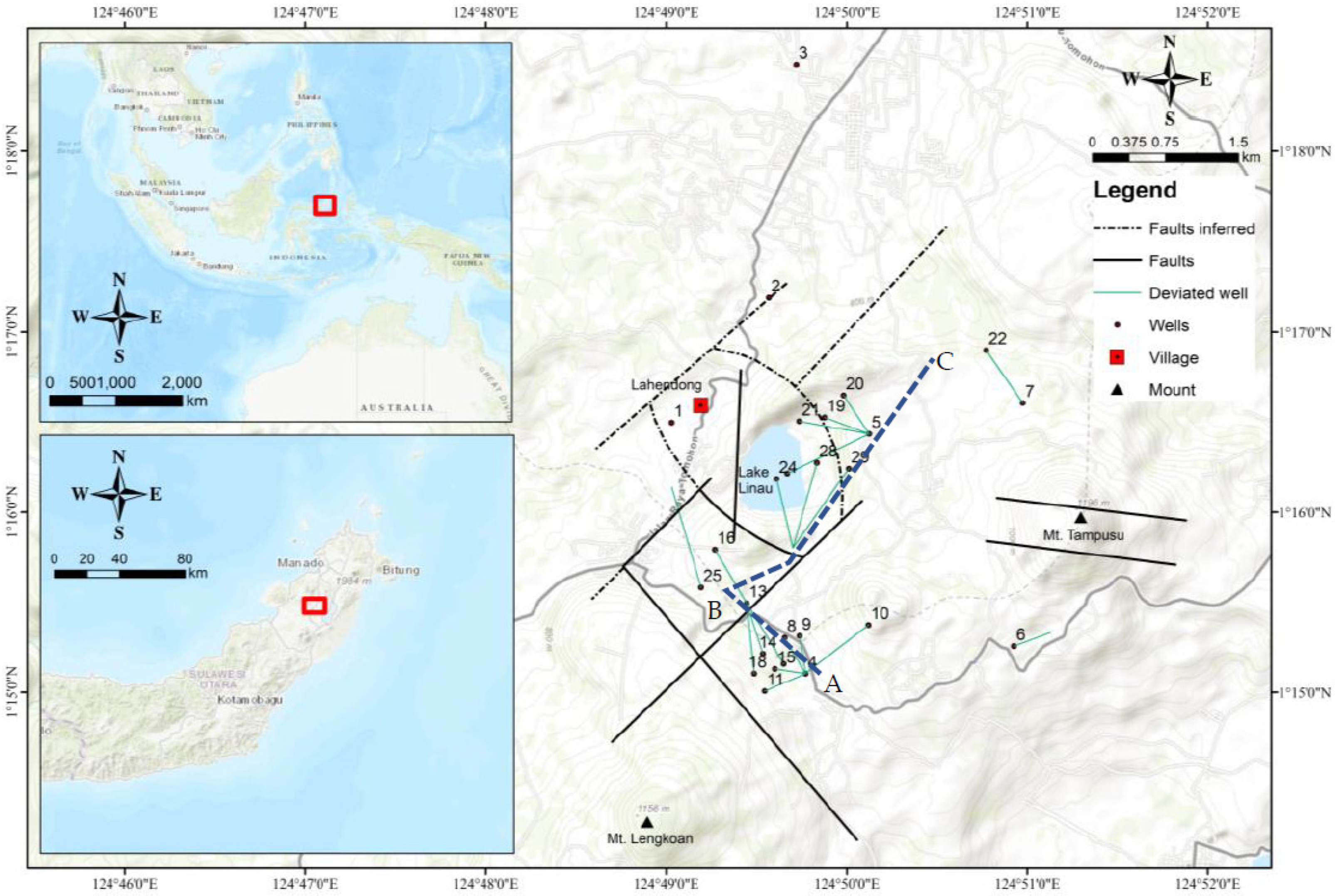
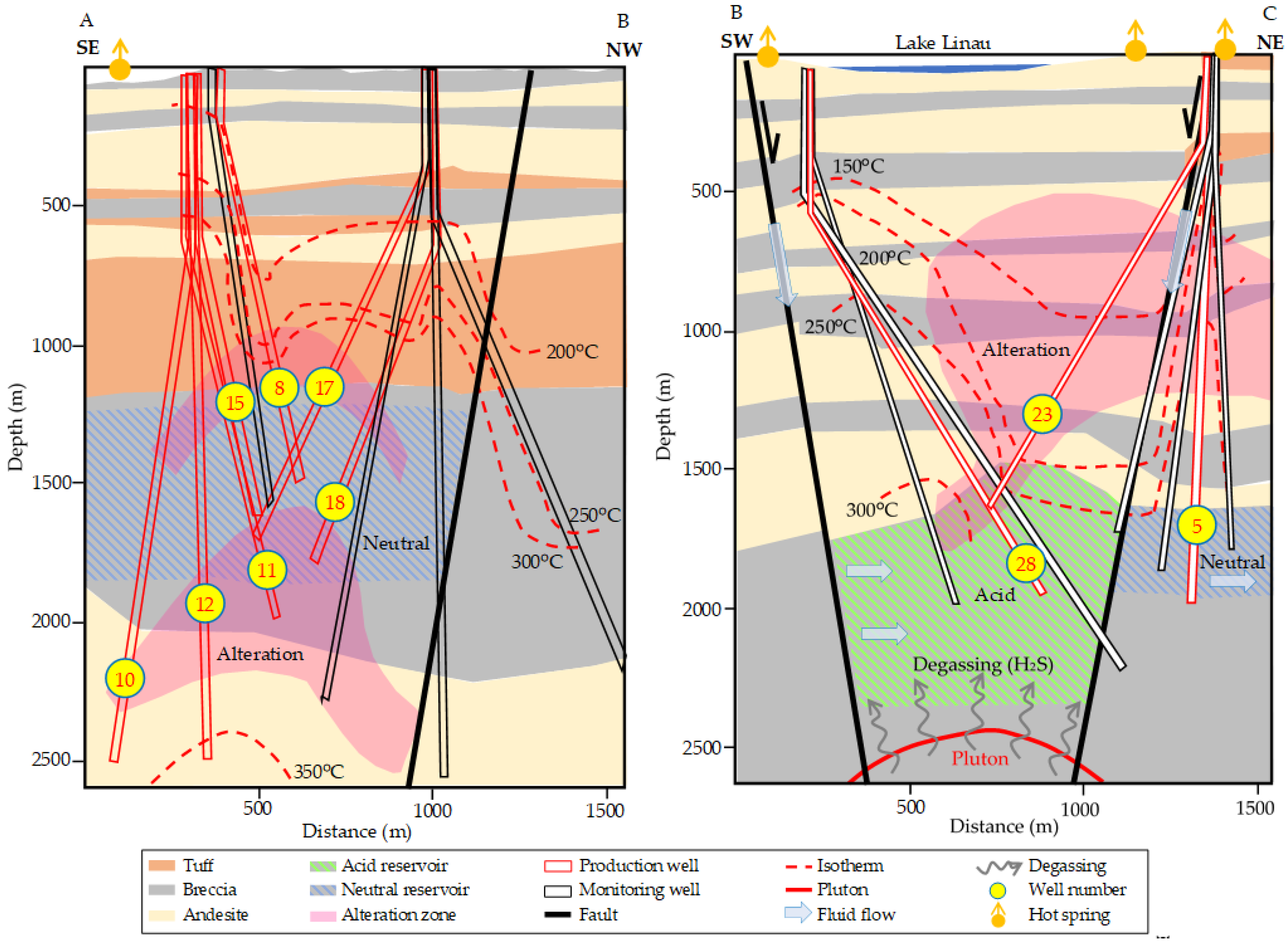
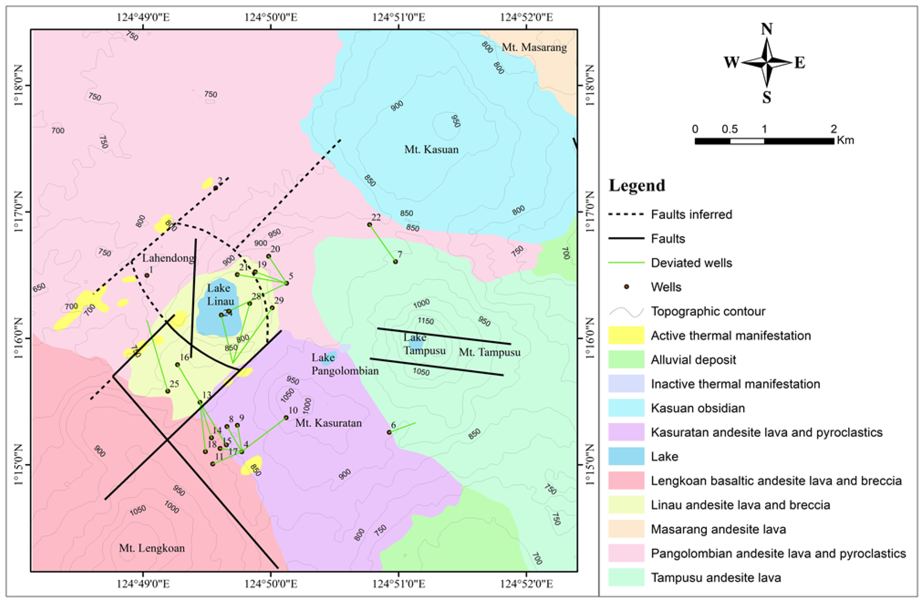
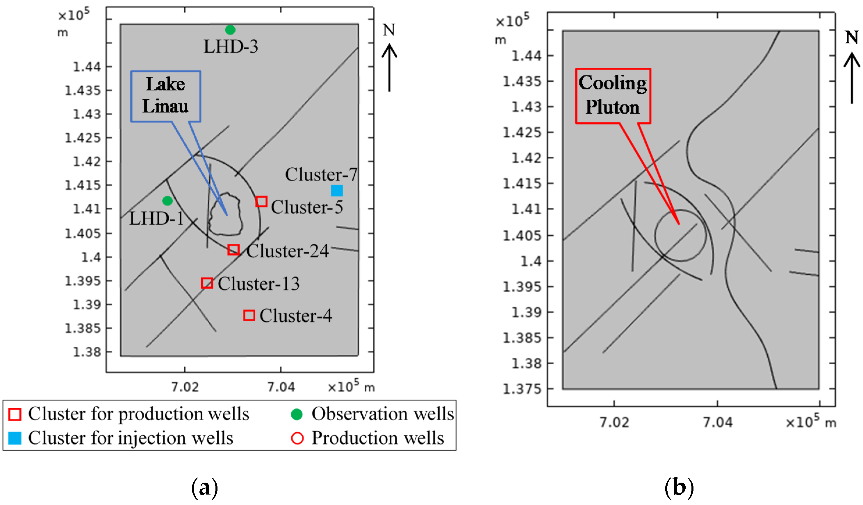
2.1. Geological
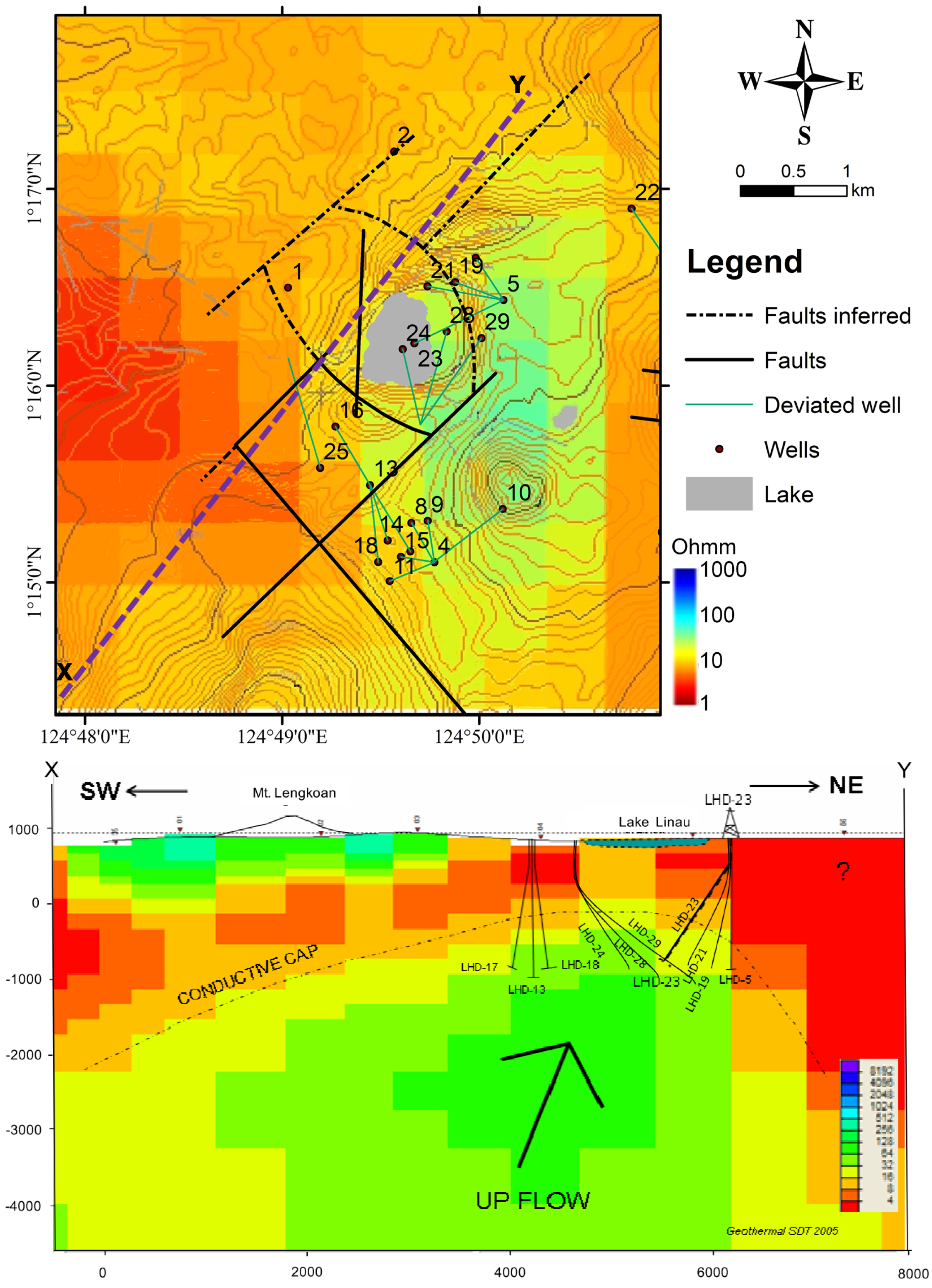
2.2. Geophysical
2.3. Well-Log Analysis
3. Methodology
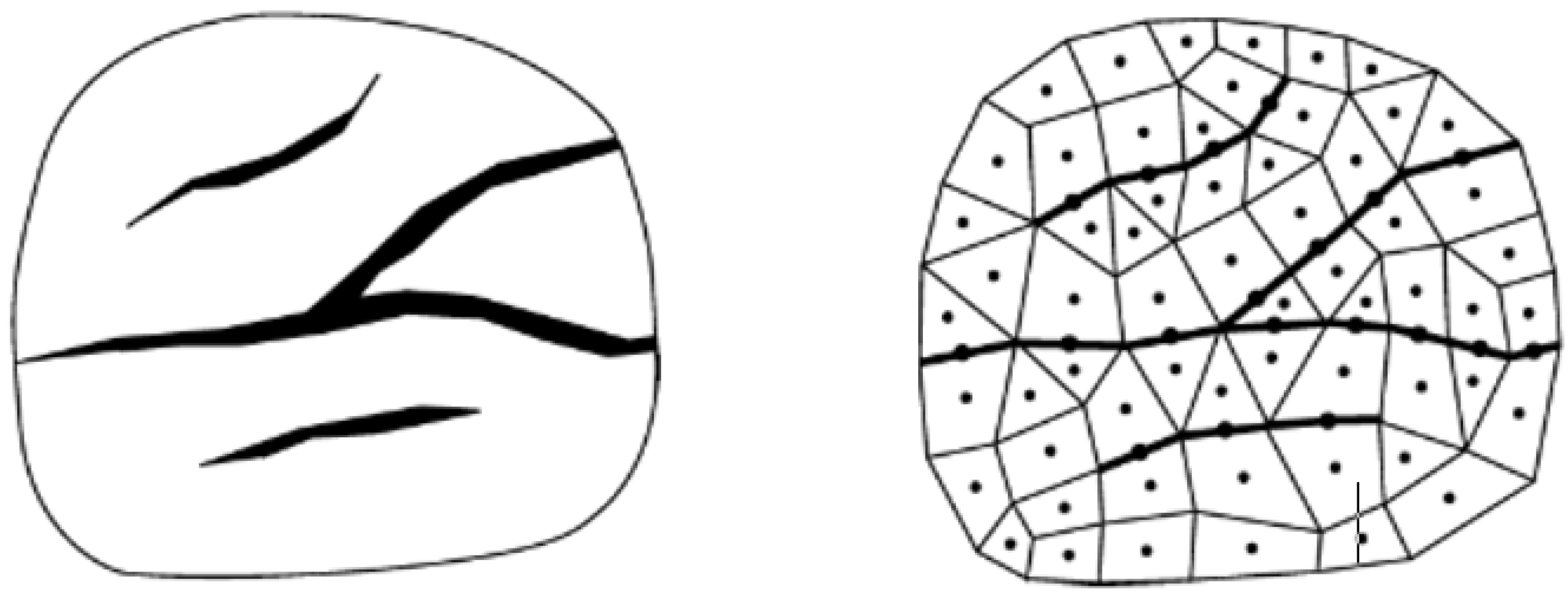
- The rock mass is treated as a 3D fractured porous media consisting of the rock matrix and discrete fractures. The discrete fracture model is applied to the fault zone in this study area.
- The fractured porous geothermal reservoir has a single-phase fluid saturation. Therefore, the water and fluid flow both in the rock matrix block and fractures comply with the Darcy’s Law.
- The model ignores the variation of fracture aperture.
- The diameter of the well is small, so that storage is negligible.
- As shown in the published paper [22], the water density and dynamic viscosity are not constant but a function of pressure and temperature.
- The density, porosity, permeability, specific heat, and thermal conductivity of the fractured porous media are assumed to be constant.
3.1. Discrete Fracture Model
3.2. Governing Equations
3.2.1. Fluid Migration
3.2.2. Rock Mass Temperature
3.2.3. Rock Mass Stress Field
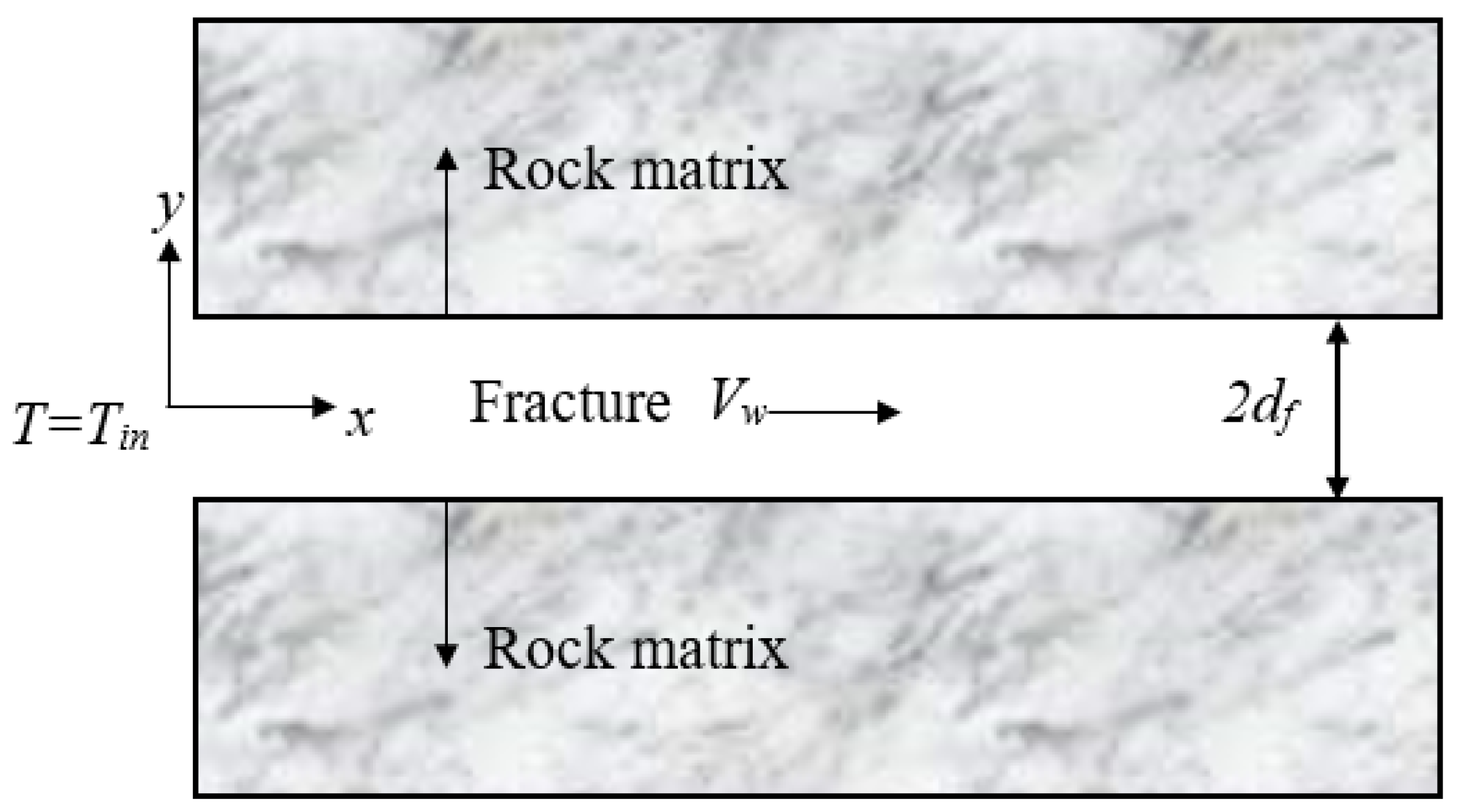
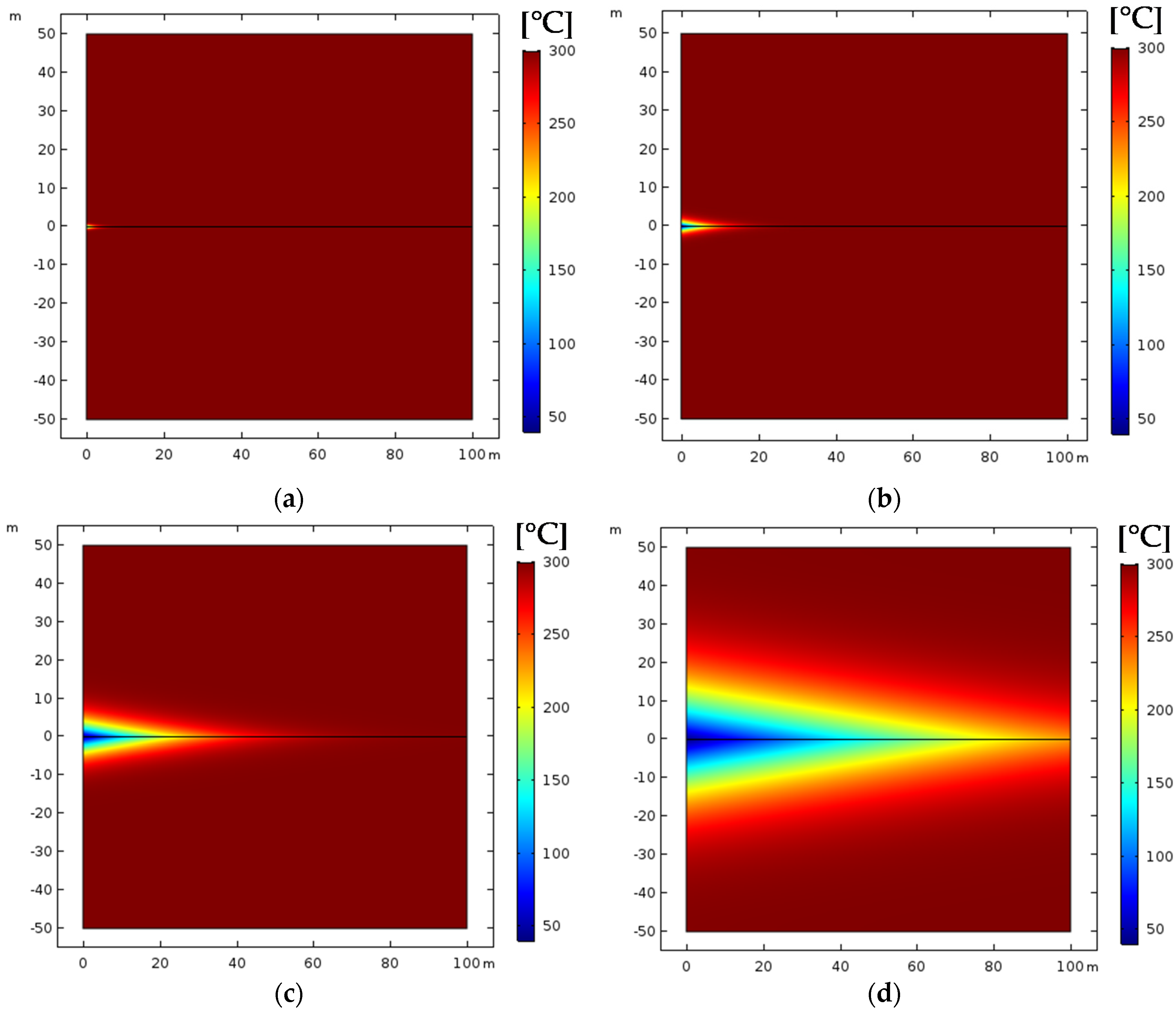
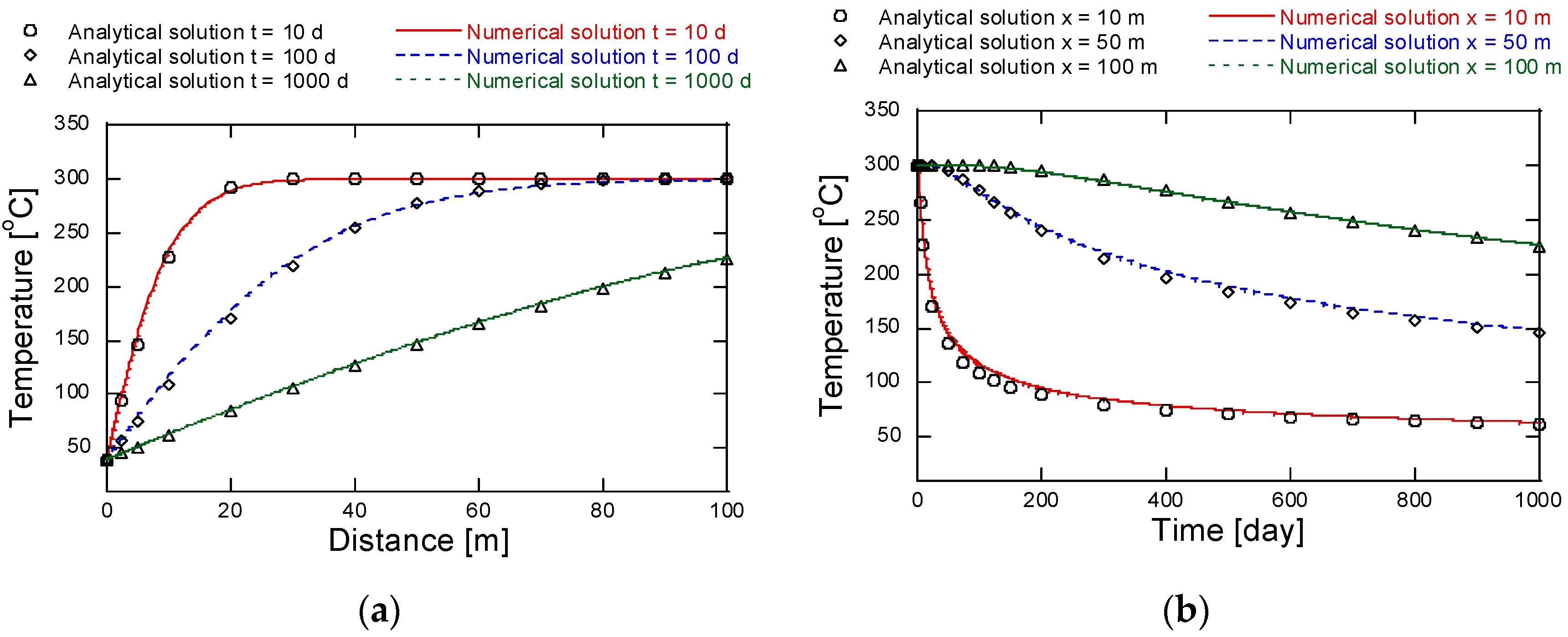
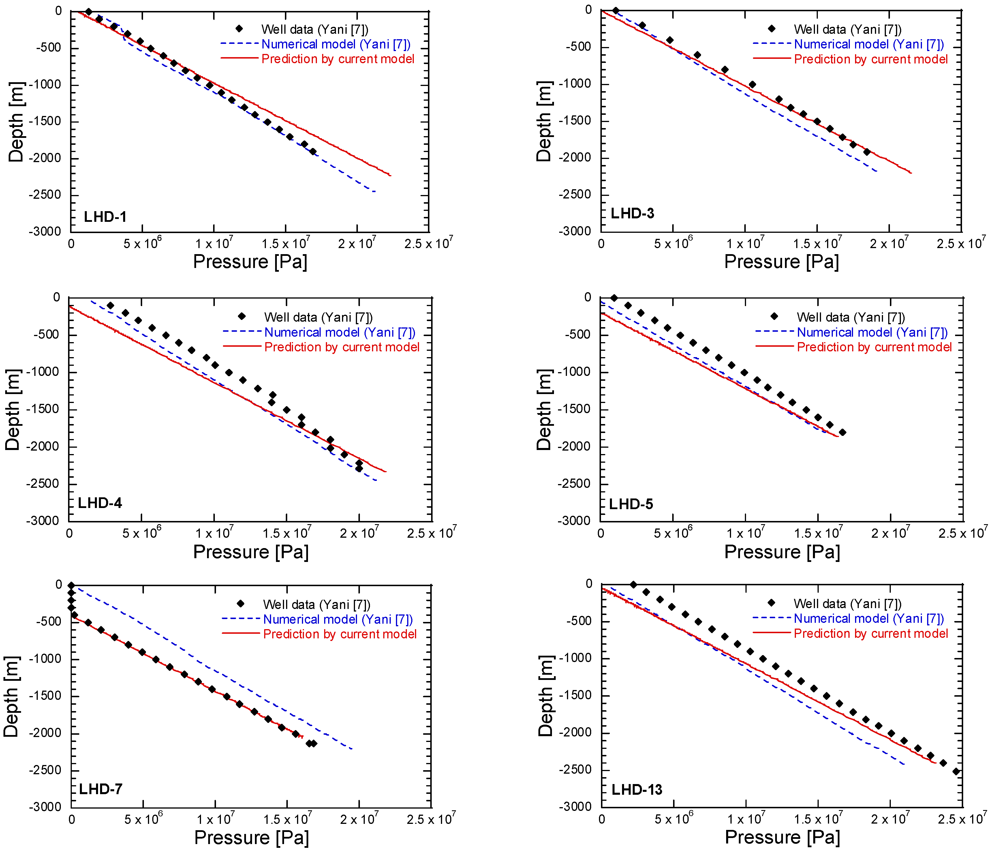
3.3. Validation and Calibration of the Numerical Model
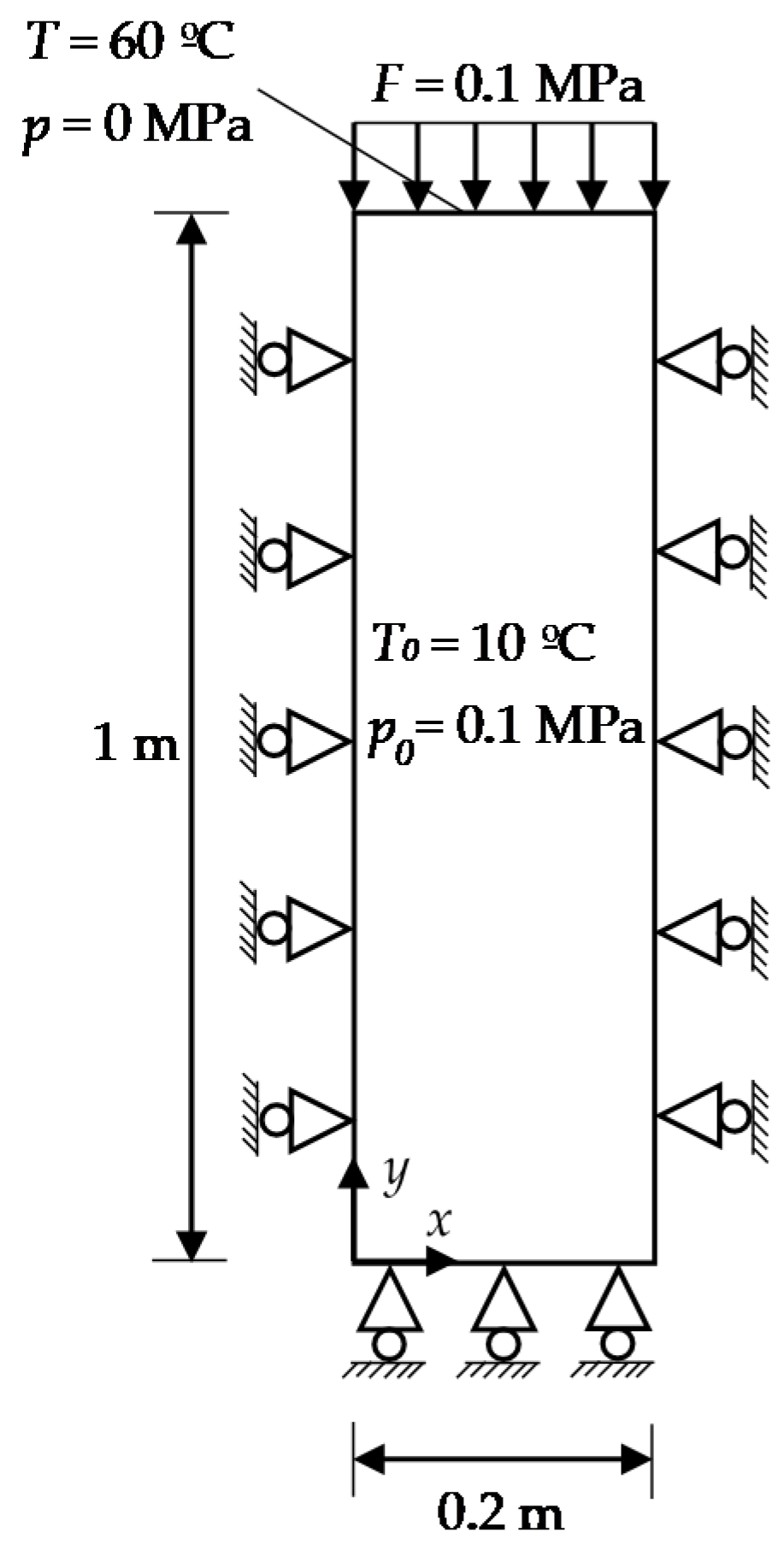
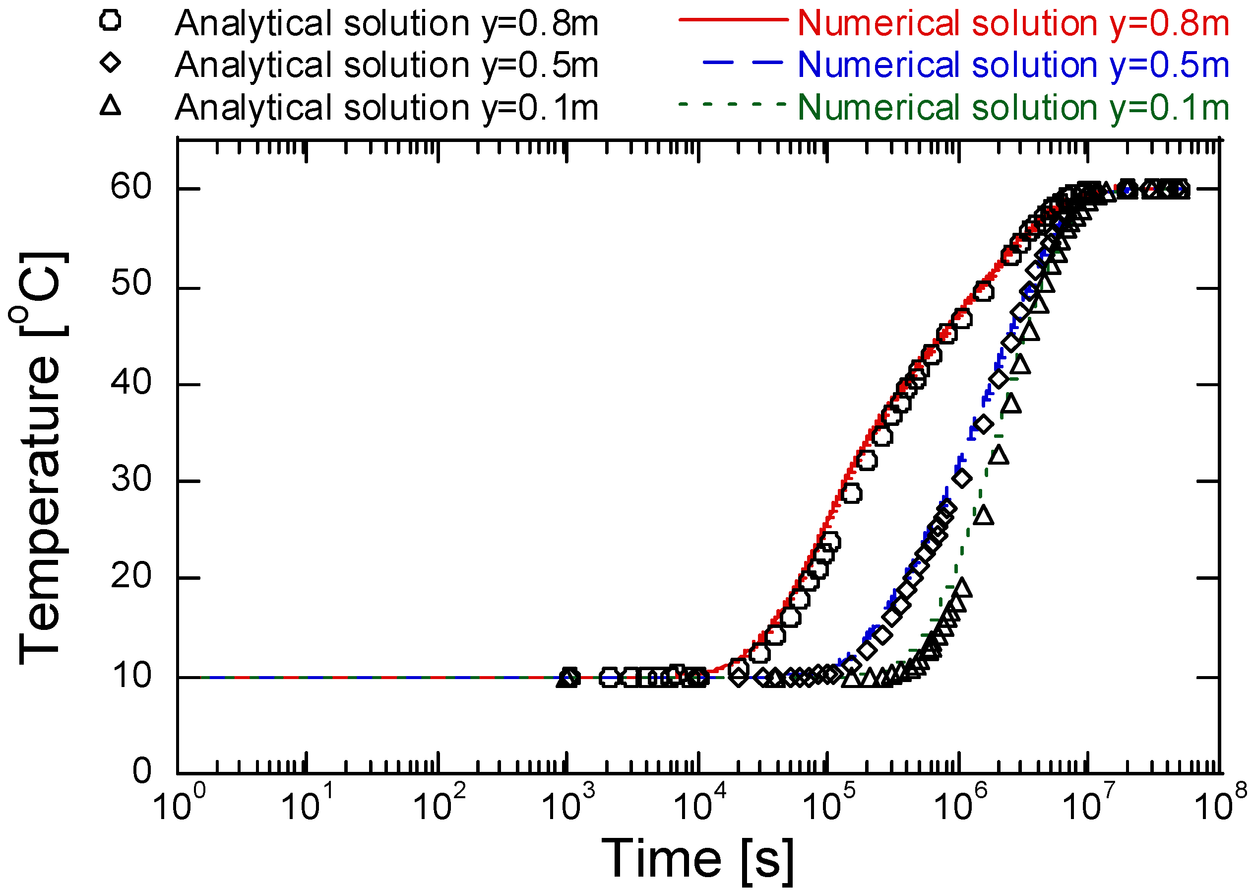
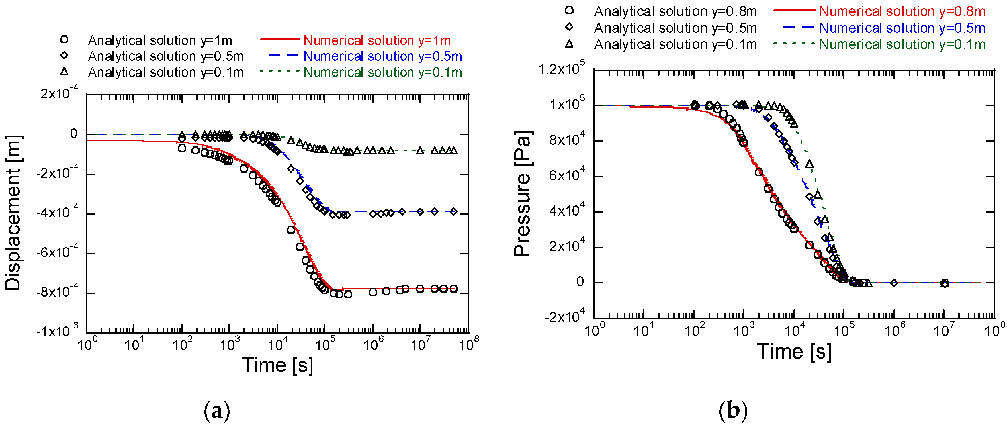
3.3.1. Validation of the TH and THM Coupling Model
3.3.2. Natural State Calibration
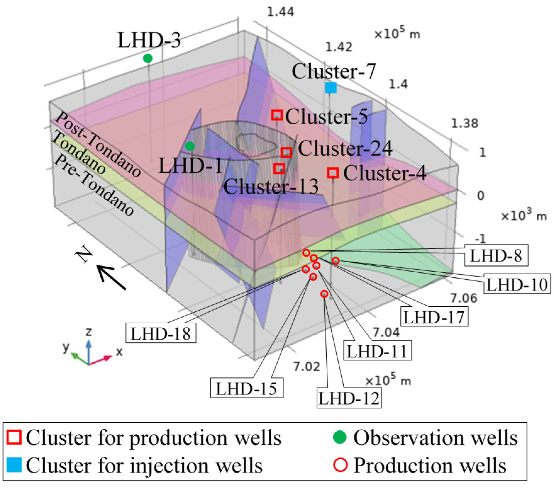
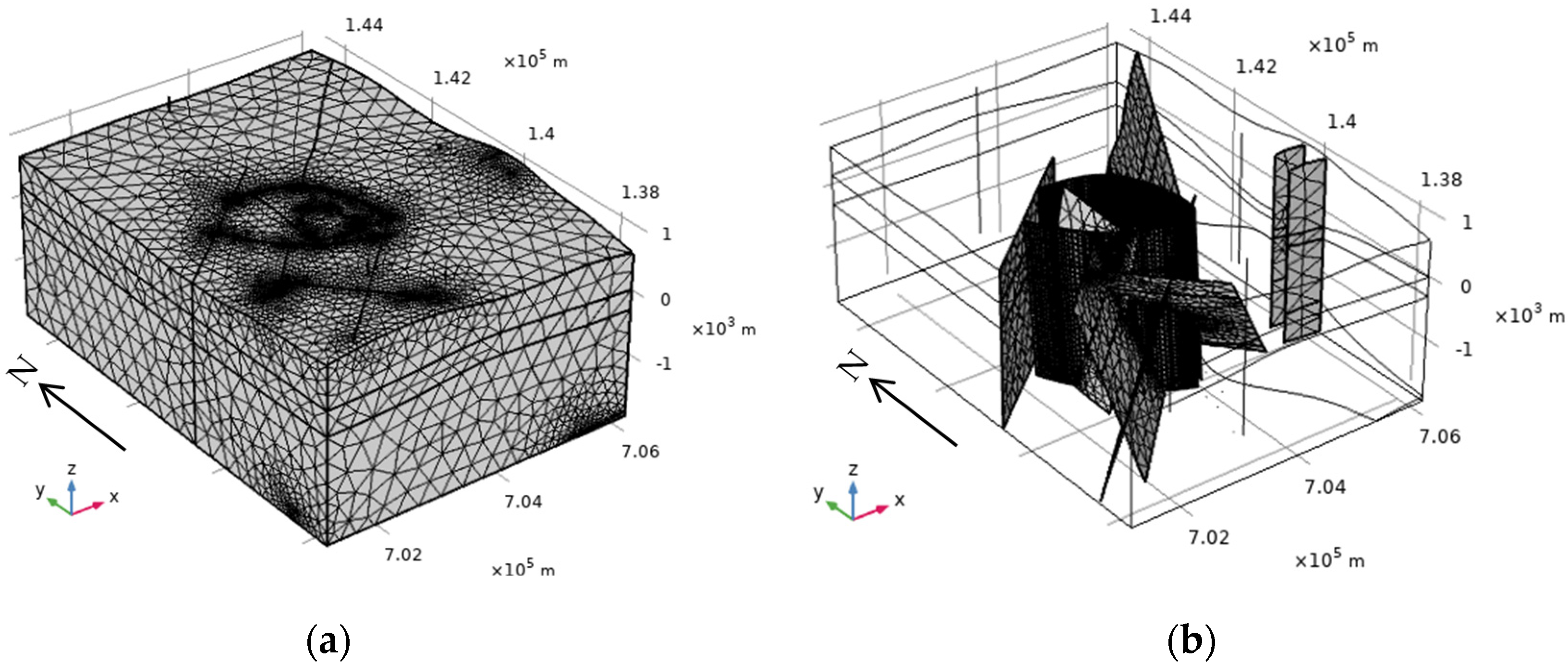
4. Computational Model
4.1. Initial and Boundary Conditions
4.2. Model Parameters
5. Results and Discussions
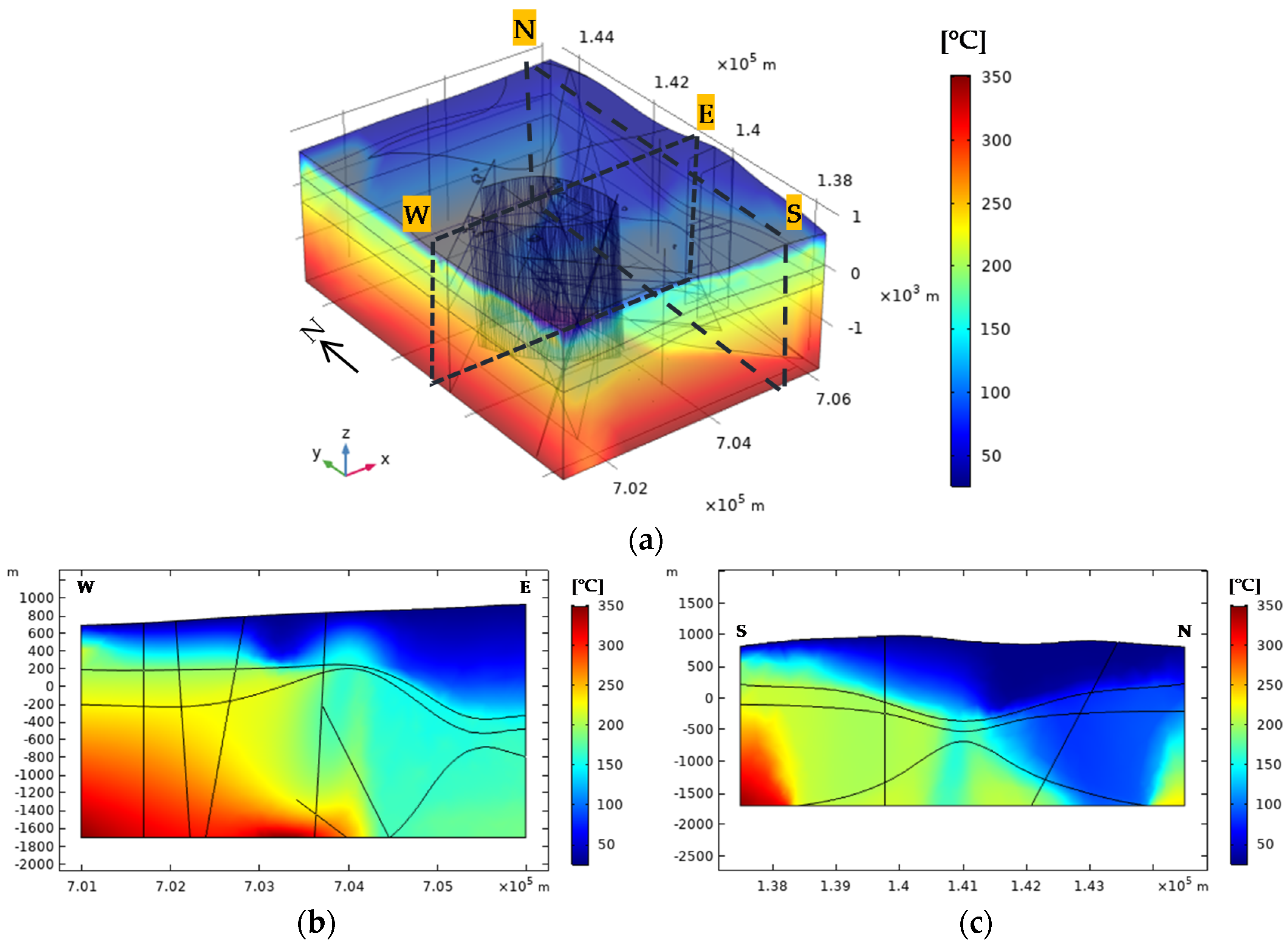
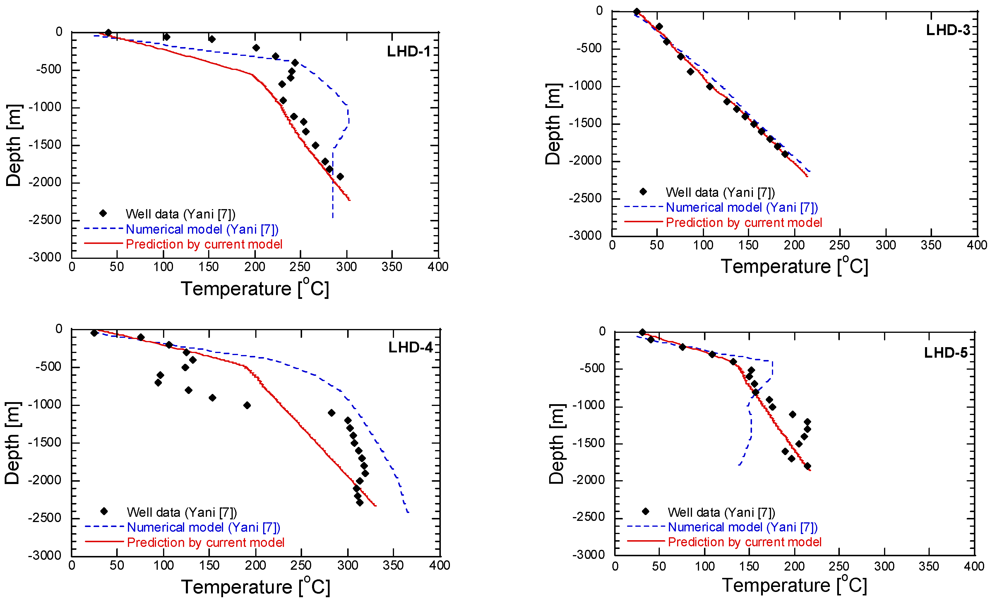
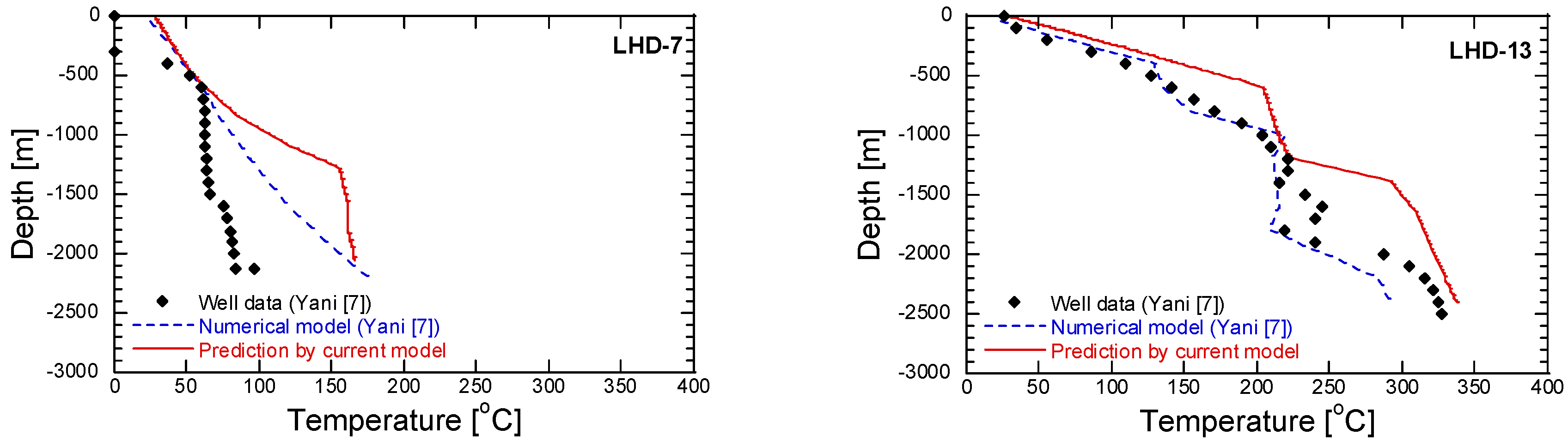
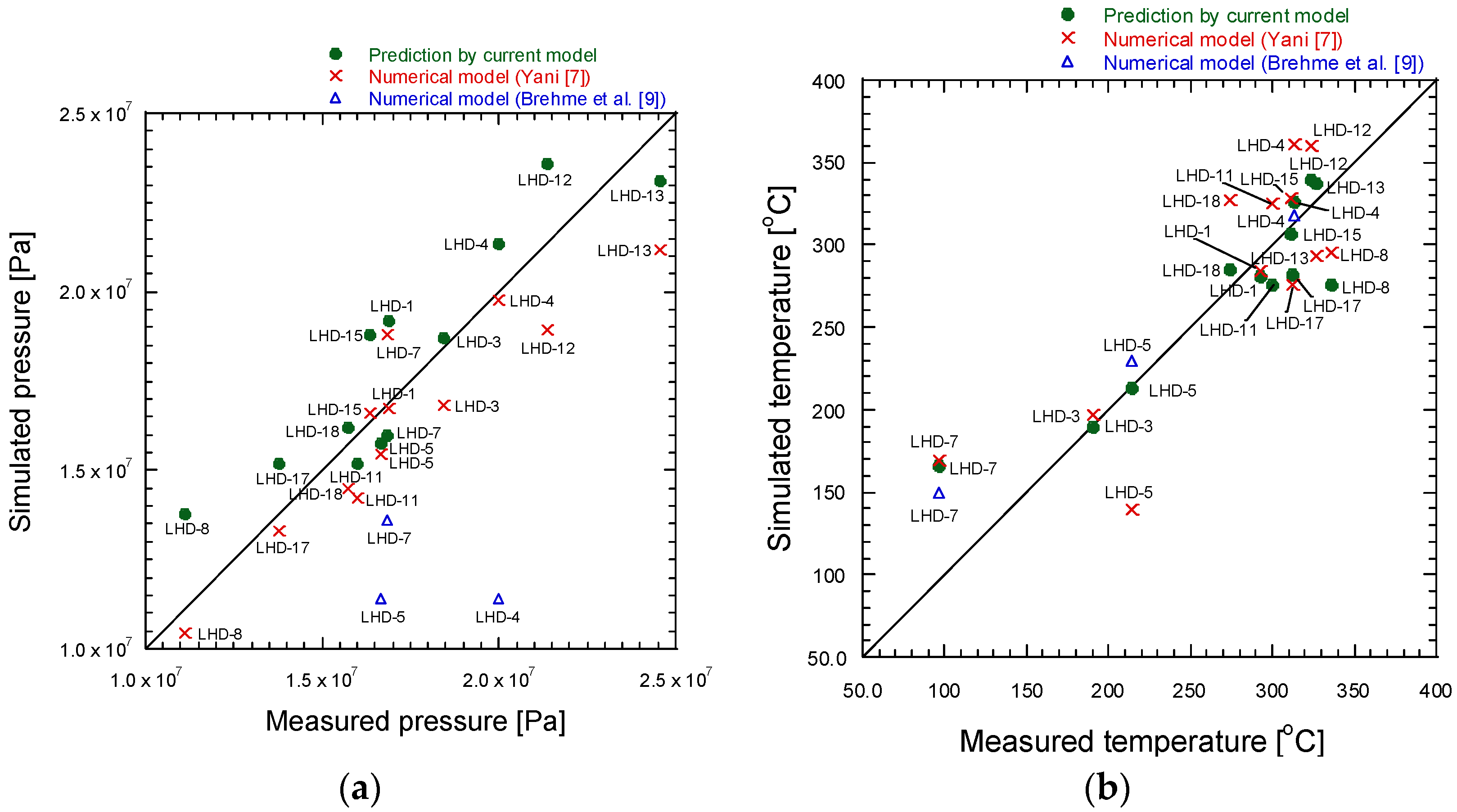
5.1. Natural State Condition
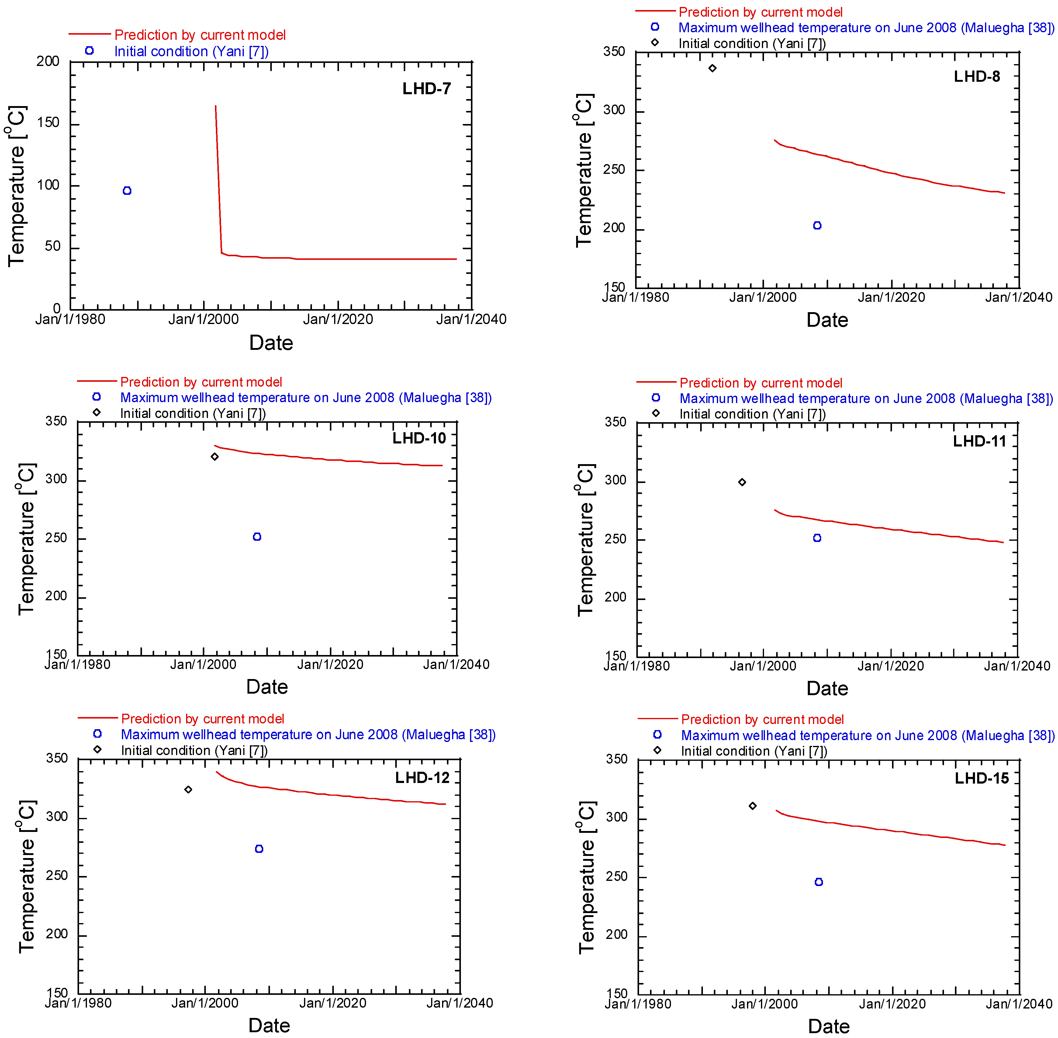
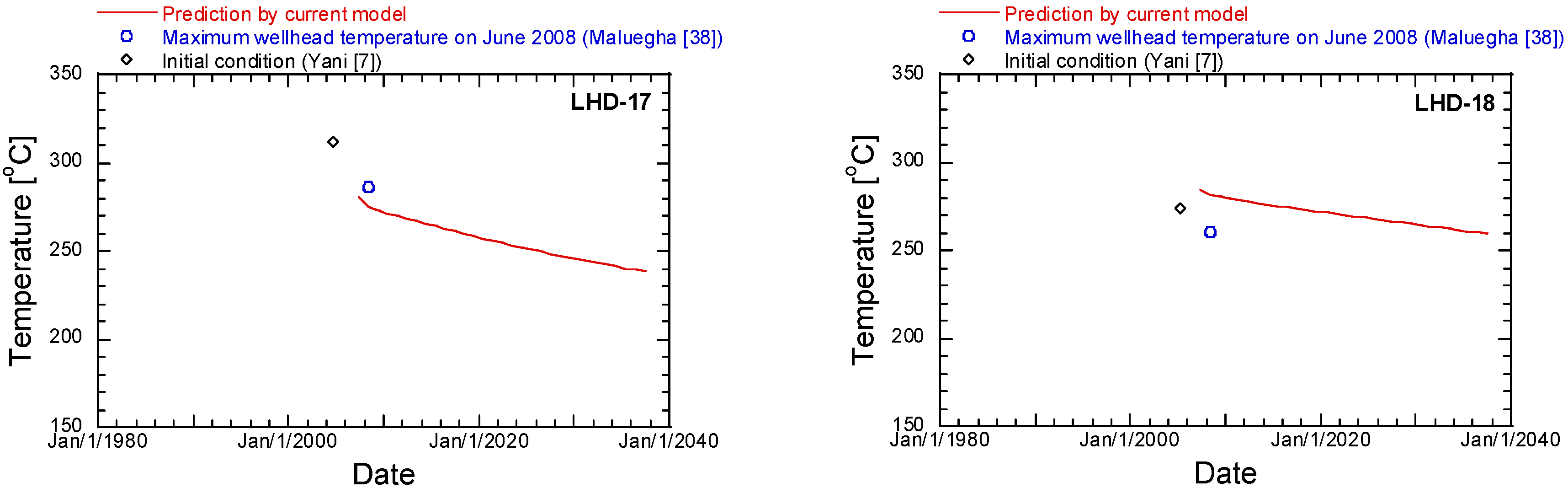
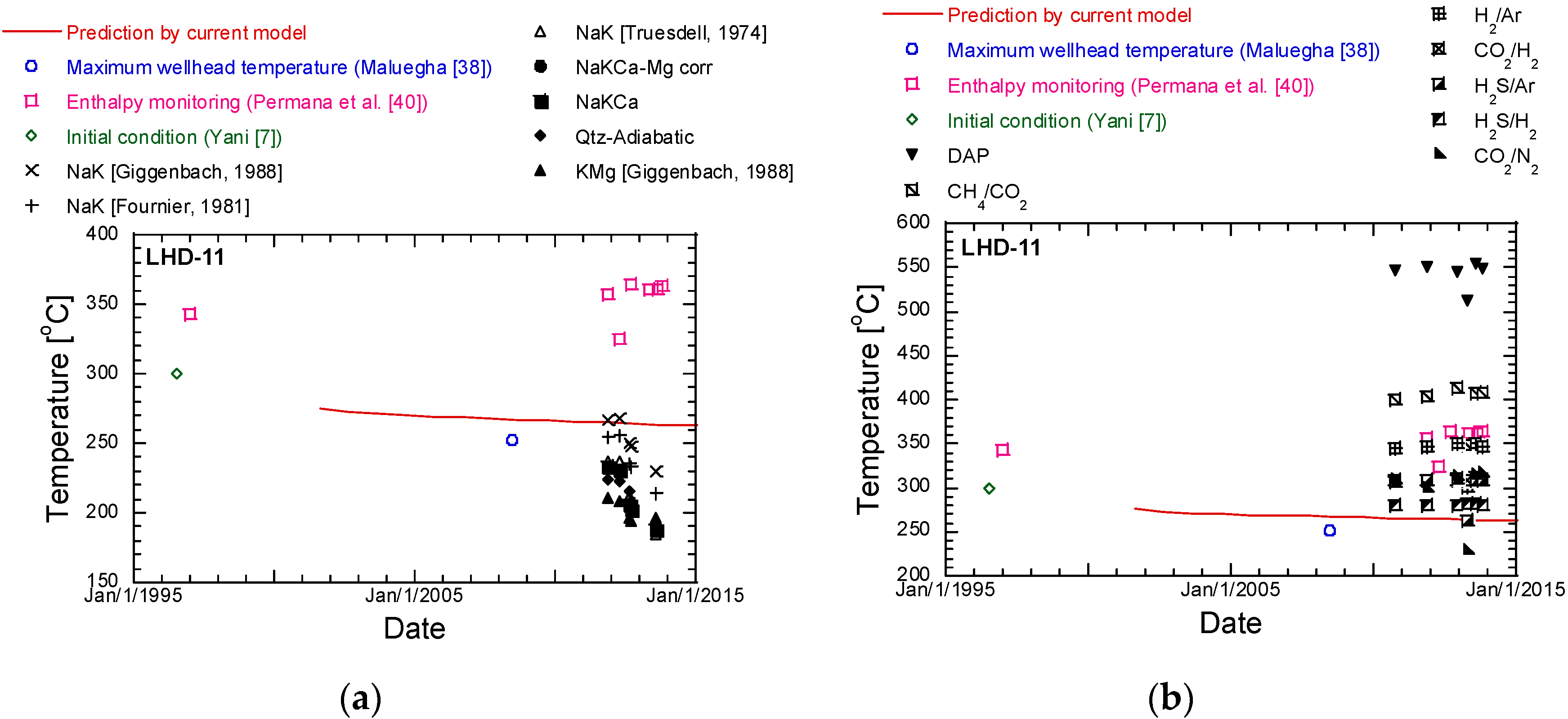
5.2. Evolution of the Reservoir Temperature
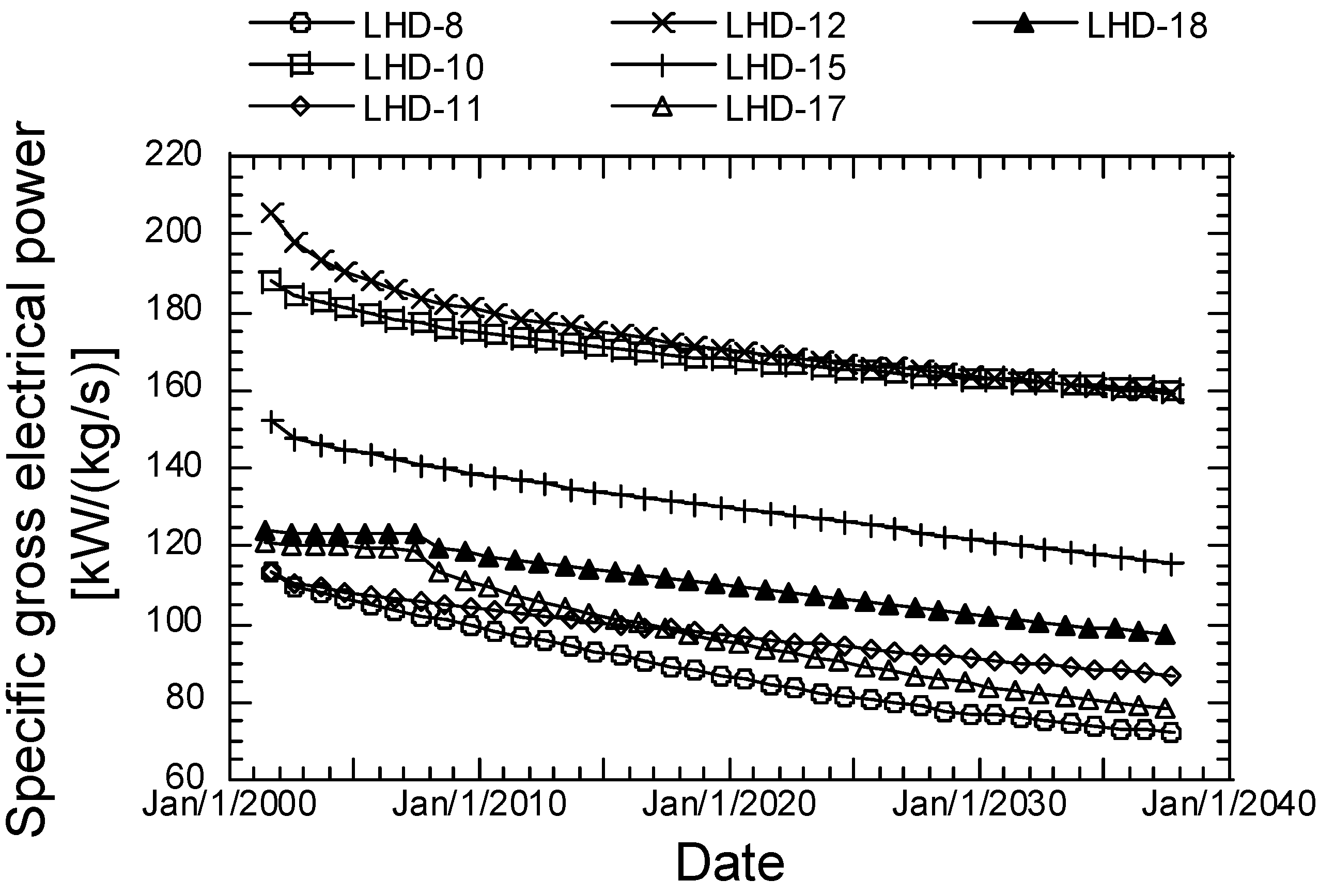
5.3. Specific Gross Electrical Power Prediction
6. Conclusions
Author Contributions
Funding
Acknowledgments
Conflicts of Interest
References
- Pambudi, N.A. Geothermal power generation in Indonesia, a country within the ring of fire: Current status, future development and policy. Renew. Sustain. Energy Rev. 2018, 81, 2893–2901. [Google Scholar] [CrossRef]
- Richter, A. The Top 10 Geothermal Countries 2018 Based on Installed Generation Capacity (MWe). Available online: https://www.thinkgeoenergy.com/the-top-10-geothermal-countries-2018-based-on-installed-generation-capacity-mwe/ (accessed on 28 April 2020).
- Kaya, E.; Zarrouk, S.J.; O’Sullivan, M.J. Reinjection in geothermal fields: A review of worldwide experience. Renew. Sustain. Energy Rev. 2011, 15, 47–68. [Google Scholar] [CrossRef]
- Rivera Diaz, A.; Kaya, E.; Zarrouk, S.J. Reinjection in geothermal fields—A worldwide review update. Renew. Sustain. Energy Rev. 2016, 53, 105–162. [Google Scholar] [CrossRef]
- Brehme, M.; Bauer, K.; Nukman, M.; Regenspurg, S. Self-organizing maps in geothermal exploration–A new approach for understanding geochemical processes and fluid evolution. J. Volcanol. Geotherm. Res. 2017, 336, 19–32. [Google Scholar] [CrossRef]
- Prabowo, T.; Yuniar, D.M.; Suryanto, S.; Silaban, M. Tracer Test Implementation and Analysis in Order to Evaluate Reinjection Effects in Lahendong Field. In Proceedings of the World Geothermal Congress 2015, Melbourne, Australia, 19–25 April 2015; pp. 1–6. [Google Scholar]
- Koestono, H. Lahendong geothermal field, Indonesia: Geothermal model based on wells LHD-23 and LHD-28. Master’s Thesis, United Nations University, Reykjavík, Iceland, 2010. [Google Scholar]
- Yani, A. Numerical Modelling of Lahendong Geothermal System, Indonesia; Geothermal Training Programme; United Nations University: Reykjavík, Iceland, 2006; pp. 547–580. [Google Scholar]
- Sumantoro, Z.Z.; Yeh, A.; O’Sullivan, J.P.; O’Sullivan, M.J. Reservoir Modelling of Lahendong Geothermal Field, Sulawesi - Indonesia. In Proceedings of the 37th New Zealand Geothermal Workshop, Taupo, New Zealand, 18–20 November 2015; pp. 1–8. [Google Scholar]
- Brehme, M.; Blöcher, G.; Cacace, M.; Kamah, Y.; Sauter, M.; Zimmermann, G. Permeability distribution in the Lahendong geothermal field: A blind fault captured by thermal–hydraulic simulation. Environ. Earth Sci. 2016, 75, 1088. [Google Scholar] [CrossRef]
- Prasetyo, F.; O’Sullivan, J.; O’Sullivan, M. Inverse Modelling of Lahendong Geothermal Field. In Proceedings of the 38th New Zealand Geothermal Workshop, Auckland, New Zealand, 23–25 November 2016; pp. 1–8. [Google Scholar]
- Danko, G.; Bahrami, D. A New T-H-M-C Model Development for Discrete-Fracture EGS Studies. GRC Trans. 2012, 36, 10. [Google Scholar]
- Yasuhara, H.; Kinoshita, N.; Ogata, S.; Cheon, D.-S.; Kishida, K. Coupled thermo-hydro-mechanical-chemical modeling by incorporating pressure solution for estimating the evolution of rock permeability. Int. J. Rock Mech. Min. Sci. 2016, 86, 104–114. [Google Scholar] [CrossRef] [Green Version]
- Ogata, S.; Yasuhara, H.; Kinoshita, N.; Cheon, D.-S.; Kishida, K. Modeling of coupled thermal-hydraulic-mechanical-chemical processes for predicting the evolution in permeability and reactive transport behavior within single rock fractures. Int. J. Rock Mech. Min. Sci. 2018, 107, 271–281. [Google Scholar] [CrossRef]
- Pandey, S.N.; Vishal, V.; Chaudhuri, A. Geothermal reservoir modeling in a coupled thermo-hydro-mechanical-chemical approach: A review. Earth-Sci. Rev. 2018, 185, 1157–1169. [Google Scholar] [CrossRef]
- Chen, B.; Song, E.; Cheng, X. Plane-Symmetrical Simulation of Flow and Heat Transport in Fractured Geological Media: A Discrete Fracture Model with Comsol. In Multiphysical Testing of Soils and Shales; Laloui, L., Ferrari, A., Eds.; Springer Series in Geomechanics and Geoengineering; Springer Berlin Heidelberg: Berlin/Heidelberg, Germany, 2013; pp. 149–154. ISBN 978-3-642-32491-8. [Google Scholar]
- Zhang, Y.; Zhao, G.-F. A global review of deep geothermal energy exploration: From a view of rock mechanics and engineering. Geomech. Geophys. Geo-Energy Geo-Resour. 2020, 6, 4. [Google Scholar] [CrossRef]
- Pandey, S.N.; Chaudhuri, A.; Kelkar, S. A coupled thermo-hydro-mechanical modeling of fracture aperture alteration and reservoir deformation during heat extraction from a geothermal reservoir. Geothermics 2017, 65, 17–31. [Google Scholar] [CrossRef]
- Guo, B.; Fu, P.; Hao, Y.; Peters, C.A.; Carrigan, C.R. Thermal drawdown-induced flow channeling in a single fracture in EGS. Geothermics 2016, 61, 46–62. [Google Scholar] [CrossRef] [Green Version]
- Slatlem Vik, H.; Salimzadeh, S.; Nick, H.M. Heat recovery from multiple-fracture enhanced geothermal systems: The effect of thermoelastic fracture interactions. Renew. Energy 2018, 121, 606–622. [Google Scholar] [CrossRef] [Green Version]
- Zhao, Y.; Feng, Z.; Feng, Z.; Yang, D.; Liang, W. THM (Thermo-hydro-mechanical) coupled mathematical model of fractured media and numerical simulation of a 3D enhanced geothermal system at 573 K and buried depth 6000–7000 M. Energy 2015, 82, 193–205. [Google Scholar] [CrossRef]
- Sun, Z.; Zhang, X.; Xu, Y.; Yao, J.; Wang, H.; Lv, S.; Sun, Z.; Huang, Y.; Cai, M.; Huang, X. Numerical simulation of the heat extraction in EGS with thermal-hydraulic-mechanical coupling method based on discrete fractures model. Energy 2017, 120, 20–33. [Google Scholar] [CrossRef]
- Yao, J.; Zhang, X.; Sun, Z.; Huang, Z.; Liu, J.; Li, Y.; Xin, Y.; Yan, X.; Liu, W. Numerical simulation of the heat extraction in 3D-EGS with thermal-hydraulic-mechanical coupling method based on discrete fractures model. Geothermics 2018, 74, 19–34. [Google Scholar] [CrossRef]
- Sun, Z.; Xin, Y.; Yao, J.; Zhang, K.; Zhuang, L.; Zhu, X.; Wang, T.; Jiang, C. Numerical Investigation on the Heat Extraction Capacity of Dual Horizontal Wells in Enhanced Geothermal Systems Based on the 3-D THM Model. Energies 2018, 11, 280. [Google Scholar] [CrossRef] [Green Version]
- Magnenet, V.; Fond, C.; Genter, A.; Schmittbuhl, J. Two-dimensional THM modelling of the large scale natural hydrothermal circulation at Soultz-sous-Forêts. Geotherm. Energy 2014, 2, 17. [Google Scholar] [CrossRef] [Green Version]
- Vallier, B.; Magnenet, V.; Schmittbuhl, J.; Fond, C. THM modeling of hydrothermal circulation at Rittershoffen geothermal site, France. Geotherm. Energy 2018, 6, 22. [Google Scholar] [CrossRef]
- Karimi-Fard, M.; Durlofsky, L.J.; Aziz, K. An Efficient Discrete-Fracture Model Applicable for General-Purpose Reservoir Simulators. SPE J. 2004, 9, 227–236. [Google Scholar] [CrossRef]
- Xu, C.; Li, P.; Lu, Z.; Liu, J.; Lu, D. Discrete fracture modeling of shale gas flow considering rock deformation. J. Nat. Gas Sci. Eng. 2018, 52, 507–514. [Google Scholar] [CrossRef]
- Utami, P. Hydrothermal Alteration and The Evolution of The Lahendong Geothermal System, North Sulawesi, Indonesia. Ph.D. Thesis, University of Auckland, Auckland, New Zealand, 2011. [Google Scholar]
- Brehme, M.; Moeck, I.; Kamah, Y.; Zimmermann, G.; Sauter, M. A hydrotectonic model of a geothermal reservoir – A study in Lahendong, Indonesia. Geothermics 2014, 51, 228–239. [Google Scholar] [CrossRef]
- Brehme, M.; Deon, F.; Haase, C.; Wiegand, B.; Kamah, Y.; Sauter, M.; Regenspurg, S. Fault controlled geochemical properties in Lahendong geothermal reservoir Indonesia. Grundwasser 2016, 21, 29–41. [Google Scholar] [CrossRef]
- Siahaan, E.E.; Soemarinda, S.; Fauzi, A.; Silitonga, T.; Azimudin, T.; Raharjo, I.B. Tectonism and Volcanism Study in the Minahasa Compartment of the North Arm of Sulawesi Related to Lahendong Geothermal Field, Indonesia. In Proceedings of the World Geothermal Congress 2005, Antalya, Turkey, 24–29 April 2005; pp. 1–5. [Google Scholar]
- Sumintadireja, P.; Sudarman, S.; Zaini, I. Lahendong Geothermal Field Boundary Based on Geological and Geophysical Data. In Proceedings of the 5th INAGA Annual Scientific Conference & Exhibitions, Yogyakarta, Indonesia, 7–10 March 2001; pp. 1–8. [Google Scholar]
- Utami, P.; Widarto, D.S.; Atmojo, J.P.; Kamah, Y.; Browne, P.R.L.; Warmada, I.W.; Bignall, G.; Chambefort, I. Hydrothermal Alteration and Evolution of the Lahendong Geothermal System. In Proceedings of the Proceedings World Geothermal Congress 2015, Melbourne, Australia, 19–25 April 2015; pp. 1–10. [Google Scholar]
- Raharjo, I.B.; Maris, V.; Wannamaker, P.E.; Chapman, D.S. Resistivity Structures of Lahendong and Kamojang Geothermal Systems Revealed from 3-D Magnetotelluric Inversions, a Comparative Study. In Proceedings of the World Geothermal Congress 2010, Bali, Indonesia, 25–29 April 2010; pp. 1–6. [Google Scholar]
- Kim, J.-G.; Deo, M.D. Finite element, discrete-fracture model for multiphase flow in porous media. AIChE J. 2000, 46, 1120–1130. [Google Scholar] [CrossRef]
- Moinfar, A.; Varavei, A.; Sepehrnoori, K.; Johns, R.T. Development of a Coupled Dual Continuum and Discrete Fracture Model for the Simulation of Unconventional Reservoirs. In Proceedings of the SPE Reservoir Simulation Symposium, Society of Petroleum Engineers, The Woodlands, TX, USA, 18–20 February 2013; pp. 1–17. [Google Scholar]
- Lauwerier, H.A. The transport of heat in an oil layer caused by the injection of hot fluid. Appl. Sci. Res. 1955, 5, 145–150. [Google Scholar] [CrossRef]
- Bai, B. One-dimensional thermal consolidation characteristics of geotechnical media under non-isothermal condition. Eng. Mech. 2005, 22, 186–191. [Google Scholar]
- Widagda, L.; Jagranatha, I.B. Recharge Calculation of Lahendong Geothermal Field in North Sulawesi-Indonesia. In Proceedings of the World Geothermal Congress 2005, Antalya, Turkey, 24–29 April 2005; pp. 1–3. [Google Scholar]
- Hattori, T. Lahendong II Geothermal Power Plant Project in Indonesia. GRC Trans. 2007, 31, 511–514. [Google Scholar]
- Silitonga, T.H.; Siahaan, E.E.; Suroso, E. A Poisson’s Ratio Distribution from Wadati Diagram as Indicator of Fracturing of Lahendong Geothermal Field, North Sulawesi, Indonesia. In Proceedings of the World Geothermal Congress 2005, Antalya, Turkey, 24–29 April 2005; pp. 1–5. [Google Scholar]
- Yoshioka, K.; Stimac, J. Geologic and Geomechanical Reservoir Simulation Modeling of High Pressure Injection, West Salak, Indonesia. In Proceedings of the World Geothermal Congress 2010, Bali, Indonesia, 25–29 April 2010; pp. 1–10. [Google Scholar]
- Maluegha, B.L. Calculation of Gross Electrical Power from the Production Wells in Lahendong Geothermal Field in North Sulawesi, Indonesia. Master’s Thesis, Murdoch University, Perth, Australia, 2010. [Google Scholar]
- Keenan, J.H.; Keyes, F.G. Thermodynamic Properties of Steam, 1st ed.; John Willey & Sons, Inc.: New York, NY, USA, 1967. [Google Scholar]
- Permana, T.; Hartanto, D.B. Geochemical Changes during 12 Year Exploitation of the Southern Reservoir Zone of Lahendong Geothermal Field, Indonesia. In Proceedings of the World Geothermal Congress 2015, Melbourne, Australia, 19–25 April 2015; pp. 1–6. [Google Scholar]
- Park, S.; Kim, K.-I.; Kwon, S.; Yoo, H.; Xie, L.; Min, K.-B.; Kim, K.Y. Development of a hydraulic stimulation simulator toolbox for enhanced geothermal system design. Renew. Energy 2018, 118, 879–895. [Google Scholar] [CrossRef]
- Ingebritsen, S.E.; Sanford, W.E.; Neuzil, C.E. Groundwater in Geologic Processes, 2nd ed.; Cambridge University Press: Cambridge, UK; New York, NY, USA, 2006; ISBN 978-0-521-60321-8. [Google Scholar]
- Carlino, S.; Troiano, A.; Di Giuseppe, M.G.; Tramelli, A.; Troise, C.; Somma, R.; De Natale, G. Exploitation of geothermal energy in active volcanic areas: A numerical modelling applied to high temperature Mofete geothermal field, at Campi Flegrei caldera (Southern Italy). Renew. Energy 2016, 87, 54–66. [Google Scholar] [CrossRef]
- DiPippo, R. Geothermal Power Plants: Principles, Applications, Case Studies and Environmental Impact; Elsevier Science: Melbourne, Australia, 2015; ISBN 978-0-08-100290-2. [Google Scholar]
- Mulyana, C.; Adiprana, R.; Saad, A.H.; Muhammad, F. The thermodynamic cycle models for geothermal power plants by considering the working fluid characteristic. AIP Conf. Proc. 2016, 1712, 020002–1–020002–7. [Google Scholar]


| Parameter | Unit | Value |
|---|---|---|
| Initial temperature | °C | 300 |
| Injection temperature | °C | 40 |
| Thermal conductivity | W/m/K | 3.5 |
| Fluid density | kg/m3 | 1000 |
| Specific heat capacity of the fluid | J/kg/K | 4200 |
| Rock density | kg/m3 | 2500 |
| Specific heat capacity of the rock | J/kg/K | 1000 |
| Fracture thickness | m | 5 10−4 |
| Fluid flow velocity in the discrete fractures | m/s | 0.01 |
| Parameter | Unit | Value |
|---|---|---|
| Fluid density | kg/m3 | 1000 |
| Soil density | kg/m3 | 2600 |
| Porosity | - | 0.4 |
| Hydraulic conductivity | m/s | 1 10−9 |
| Thermal conductivity | W/m/K | 0.5 |
| Specific heat capacity of the fluid | J/kg/K | 4200 |
| Specific heat capacity of the soil | J/kg/K | 800 |
| Elastic modulus of the soil | MPa | 60 |
| Poisson’s ratio | - | 0.4 |
| Thermal expansion coefficient | - | 3 10−7 |
| Biot-Willis coefficient | - | 1.0 |
| Coefficient of compressibility | Pa−1 | 1.1 10−10 |
| Type | Location | |||||
|---|---|---|---|---|---|---|
| Bottom | Lake | Northern | Southern | Western | Eastern | |
| Temperature, °C | 91-0.0853z | 213-0.0801z | 213-0.0801z | 59-0.0199z | ||
| Hydraulic head 1,2, m | 767 | 772 | 809 | 837 | 506 | |
| Heat flux 2, mW/m2 | 100 | |||||
| Parameter | Unit | Value | |||
|---|---|---|---|---|---|
| Post-Tondano Formation | Tondano Formation | Pre-Tondano Formation | Fracture | ||
| Density 1 | kg/m3 | 2630 | 2320 | 2490 | 1800 |
| Porosity 1 | 0.05 | 0.12 | 0.11 | 0.2 | |
| Permeability (x, y, z) 2 | m2 | 2.1 10−15, 2.1 10−15, 2.1 10−13 | 2.3 10−13, 2.3 10−13, 2.3 10−11 | 1 10−17, 2 10−15, 5 10−13 | 7 10−15, 2 10−15, 2 10−15 |
| Specific heat 2 | J/kg/K | 1000 | 1000 | 1000 | 1000 |
| Heat conductivity 3 | W/m/K | 2.2 | 2.5 | 2.1 | 1.8 |
| Elastic modulus | GPa | 45 | 50 | 65 | |
| Poisson’s ratio 4 | 0.4 | 0.35 | 0.3 | ||
© 2020 by the authors. Licensee MDPI, Basel, Switzerland. This article is an open access article distributed under the terms and conditions of the Creative Commons Attribution (CC BY) license (http://creativecommons.org/licenses/by/4.0/).
Share and Cite
Qarinur, M.; Ogata, S.; Kinoshita, N.; Yasuhara, H. Predictions of Rock Temperature Evolution at the Lahendong Geothermal Field by Coupled Numerical Model with Discrete Fracture Model Scheme. Energies 2020, 13, 3282. https://doi.org/10.3390/en13123282
Qarinur M, Ogata S, Kinoshita N, Yasuhara H. Predictions of Rock Temperature Evolution at the Lahendong Geothermal Field by Coupled Numerical Model with Discrete Fracture Model Scheme. Energies. 2020; 13(12):3282. https://doi.org/10.3390/en13123282
Chicago/Turabian StyleQarinur, Muhammad, Sho Ogata, Naoki Kinoshita, and Hideaki Yasuhara. 2020. "Predictions of Rock Temperature Evolution at the Lahendong Geothermal Field by Coupled Numerical Model with Discrete Fracture Model Scheme" Energies 13, no. 12: 3282. https://doi.org/10.3390/en13123282