1. Introduction
Heat transfer in natural convective flows arising in cavities due to temperature gradients have been widely investigated for their importance in a wide range of engineering applications, ranging from the cooling of electronic equipment and nuclear reactors and thermal-fluid dynamic behavior of solar energy collectors to the optimization of thermal insulation in buildings [
1]. The cavities can be either enclosures [
1,
2,
3,
4,
5], not admitting mass transfer at the boundaries, or vented cavities, in which a mass transfer is established typically between an inlet and an outlet section [
6,
7,
8].
When dealing with natural convection in enclosures, significant interest is focused on the investigation of the boundary layer for specific geometries. With respect to the direction of the temperature gradient determined by the imposed boundary conditions, studies may be divided into two main groups, i.e., enclosures differentially heated on the sidewalls, and enclosures heated from the bottom and cooled from the top [
2]. Regarding the geometries, rectangular and square enclosures are the most extensively analyzed [
3], though some attention has been paid to triangular [
9], trapezoidal [
10,
11], complex structures [
12], or to annular enclosures [
13]. A relevant interest exists towards the assessment of analytical solutions able to describe both the temperature and the velocity profiles, subsequently validated through comparison with experimental observations or numerical simulations. It is worth noting that, though analytical models represent approximated solutions of the governing equations, whose validity is typically restricted to the cases of homogeneous and stationary flows obtained from the application of substantial simplifications of both the imposed boundary conditions and the enclosure’s geometry, they benefit from several advantages. In fact, within their range of validity, analytical models can be easily implemented to obtain a generalized view of thermal and velocity fields, require less input data, and have a negligible computational effort, compared to numerical models. On the other hand, even if the accuracy and predictability of numerical models are unquestionable, they require a formulation tailored to the specific geometry and to the imposed boundary conditions; moreover, their reliability must be validated through comparison with benchmark cases derived from experimental observations. Hence, analytical models can still be considered useful tools to gain awareness on the temperature, velocity, and pressure fields, as well as to formulate suitable correlations among the physical parameters characterizing the fluid flow.
Numerical and experimental studies for rectangular enclosures with two horizontal adiabatic walls and two vertical isothermal walls were studied for both square and slender cavities [
14,
15,
16,
17], and for inclined geometries [
1,
18]. Numerical models are also developed for enclosures in which one wall is heated and the other is cooled with uniform heat fluxes [
19], or for parallel plate vertical channels with asymmetric wall heat fluxes or asymmetric wall temperatures [
20]. Beyond these numerical studies, a significant part of scientific literature focused on the development of analytical models to describe natural convective flows, thus confirming the previous underlined importance of dealing with analytical solutions. Among these contributions, Batchelor [
21] proposed a theoretical study aiming at determining the heat transfer rate between two isothermally and differentially heated vertical walls. Results evidenced the flow dependence on the aspect ratio of the enclosure and on the Prandtl and Rayleigh numbers. Philips [
22] proposed an alternative analytical model for a vertical rectangular enclosure with vertical walls kept at different temperatures and adiabatic horizontal walls. The same configuration is studied by Gill [
23], who developed an approximate solution for the boundary-layer free-convection regime valid for large values of the Prandtl number. Notably, Gill’s solution contains two arbitrary constraints, consisting in impermeability conditions and top and bottom walls symmetry. An alternative approach to determine the arbitrary constants of the Gill’s solution was proposed by Bejan [
24], who proposed the evaluation of the net upward energy flow, assumed to be nil at the top and bottom boundaries of the enclosures, and derived Nusselt number correlations with the enclosure’s aspect ratio and the Rayleigh number.
Going forward with the review of the analytical studies, Kimura and Bejan [
25] investigated the boundary layer regime that develops within rectangular enclosures with adiabatic horizontal walls and vertical walls subjected to constant and uniform heating, and, respectively, cooling specific heat flux. Results evidenced that the boundary layer thickness is independent of the vertical coordinates. In addition, the core is motionless and temperatures at the vertical walls vary linearly in the vertical direction, with the same gradient observed for the temperature profile at the core of the cavity. The authors also derived the analytical expression of the Nusselt number, which depends on both the Rayleigh number and the aspect ratio, and used numerical simulations to confirm the validity of this solution. Rekha and Jawali [
26] proposed an analytical model to study the boundary layer convection with the same boundary condition of [
25], but for an inclined enclosure. Results are in agreement with those reported in [
25]. Jiracheewanun et al. [
27] assumed the same boundary conditions, and derived the analytical solution by integrating the energy equation over the control volume, and compared the results with the correspondent numerical solution, obtaining good agreements for slender enclosures over the entire range of Rayleigh numbers considered. Similarly, Kassemi [
28] studied the natural convection for an enclosure, but with an aspect ratio smaller than, or equal to, unity, and for high values of the Rayleigh number. The author developed a model based on linearization techniques and analytical iterations to find the approximate solutions for the velocity and temperature fields.
Lietzke [
29] presented a theoretical investigation of the heat transfer between two parallel vertical plates, uniformly heated and cooled, respectively. The equations of the velocity and temperature profiles and the ratio between the actual temperature drop and that for pure conduction were developed, and results of analytical calculations were then compared to experimental results. Mac Gregor and Emery [
30] investigated the free convection through vertical plane layers under both isothermal and constant heat flux wall conditions for different values of the Prandtl, Grashof, and Rayleigh numbers. Yao [
31] assessed an analytical solution for the free and forced convection in the entry region of a heated vertical channel under both constant temperatures and constant heat flux conditions along the walls. Similarly, but including the effect of viscous dissipation, Barletta [
32] studied the fully developed combined forced and free convection in a vertical channel with prescribed wall heat fluxes.
In the stream of the previous analytical studies, this study aims at analyzing the natural convection in a rectangular closed enclosure with vertical walls differentially heated by an imposed heat flux and adiabatic horizontal walls. An analytical model is developed to define the expressions of both the velocity and temperature profiles, and to derive a correlation for the Nusselt number. Unlike [
25,
26], no restriction is assumed to the boundary layer regime within the cavity; moreover, the analytical model does not assume a priori restrictions on the aspect ratio, as in [
27,
28,
29], and its validity with respect to this parameter is assessed, afterwards, through comparison with numerical results. Finally, the analytical solution is compared with the one obtained with the aim of numerical simulations, and results are discussed.
The system description, as well as the definition of the analytical model, is presented in
Section 2. Subsequently, the derived analytical solution is presented in
Section 3; finally,
Section 4 compares the results of the analytical model with numerical simulations, in order to test the validity of the developed model.
2. Problem Definition and Governing Equations
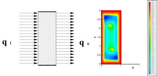
The present study considers a closed rectangular enclosure of height H and length L, filled by a fluid, with adiabatic horizontal walls and imposed heat fluxes at the vertical walls. The system geometry is reported in
Figure 1.
The following assumptions apply to the system:
The fluid is Newtonian.
The flow is two-dimensional and laminar.
The regime is stationary.
Constant material properties.
Boussinesq’s hypothesis for density holds in the whole range of operations considered, i.e.,
The energy dissipated by viscous stress can be neglected.
On this basis, the following governing equations for the conservation of mass, momentum, and energy at every point in the enclosure are obtained:
where
is the density of the fluid,
is the thermal conductivity,
is the absolute temperature,
is the pressure,
is the kinematic viscosity,
is the acceleration due to gravity,
is the velocity of the fluid, and
is the specific heat at constant pressure. The subscript “
” refers to the values assumed at the reference temperature of
.
The vertical walls are characterized by imposed heat fluxes, and the horizontal walls are adiabatic; i.e., the following thermal boundary conditions hold:
Additional boundary conditions on all solid walls for the velocity fields are ; and being the velocity components along and , respectively.
To solve the mass, momentum, and energy equations defined in Equations (1)–(3), the dimensionless variables listed in the nomenclature are applied to the problem. As a result, the obtained explicit nondimensional equations are now expressed as:
The momentum equations in Equations (7) and (8), respectively for the
and the
-direction, may be reformulated as:
Equation (10) is then expressed as:
in which the Prandtl number is
, and the Rayleigh number is
.
Similarly, the dimensionless energy equation in Equation (9) becomes:
When stationary conditions are considered, as in the following sections of the present study, the time dependent terms in the previous equations drop out. In order to quantify the convective heat transfer across the boundary system and to compare it to the heat transfer due to conduction, it is usual to refer to the Nusselt number
:
In Equation (13),
is the convective heat transfer coefficient, and
is the thermal conductivity of the fluid. For the aim of the present study, it is assumed that the conductivity of the fluid is known, while the convective heat transfer coefficient has to be calculated. According to the Fourier’s law for the determination of the heat transfer at the wall, and evaluating the contribution of the heat exchanged by convection in the system, the thermal conductivity
is:
Therefore, the Nusselt number may be expressed in its general form as:
By multiplying and by dividing for the quantity
, the differential expression for the local Nusselt number is attained as a function of the dimensionless temperature. Thus:
With the boundary condition of imposed heat flux on the walls, Equation (16) becomes:
3. Analytical Solution
As the spatial temperature and velocity fields within the enclosure depend on the geometry of the cavity and on the imposed thermal boundary conditions, as reported in [
25,
26,
27,
28,
29], the assessment of their analytical description depends on simplifying assumptions on the shapes of their profiles. Therefore, in order to achieve a systematic view of the dependence of the temperature and velocity profiles on the aspect ratio and on the
number, as well as a corresponding set of reference ranges of variation of these profiles, a series of preliminary numerical simulations were carried out. The system was numerically solved by means of a finite volume code; the TRIO-EF developed at the French Atomic Energy Center in Saclay by Magnaud et al. [
33]. The domain has been modelled by choosing a quadrangular elements mesh for the velocity components and using a staggered grid as setting for the temperature and pressure. Three iterative methods have been adopted, the ADI (alternating direction implicit) method for the resolution of the generic transport equation, the THOMAS algorithm for the resolution of the algebraic equations, and the SIMPLER (semi-implicit method for the pressure linked equations revised) for the velocity correction through a pressure-correction equation. The numerical code used in this study for solving the full elliptical governing equations was previously validated by comparison with other similar cases of natural convection flows of air in cavities with differentially heated vertical walls and adiabatic horizontal walls, as in De Vahl Davis [
33] and Le Quéré [
34]. The values of the mean Nusselt number
were obtained for different values of
on different grids, and they have been again compared with the numerical values of [
34,
35].
Table 1 reports the mean
scaled by
calculated in the present study and the corresponding values calculated in [
34,
35]. The reference values are reported for
10
6 [
34] and for
10
8 [
35]. Results are in good agreement, with a maximum relative error of 2%.
To determine the grid size, ensuring the accuracy of the solution, simulations were conducted on an increasingly finer grid size distribution; a uniform mesh size with at least (64, 64) control volumes in the
and
direction was selected, as it ensures satisfactory accuracy of the solution. Numerical simulations were conducted for aspect ratios between 1 (square cavities) and 20 (rectangular and increasingly slenderer enclosures), and with
and
. In particular, for the scopes of the present study, the square cavity with
was considered as the limiting case, whereas for growing aspect ratio, the cavities are vertical rectangular enclosures of increasing slenderness; cavities with aspect ratio
were not considered, as they are beyond the scope of the present study.
Table 2 reports the mean values of the magnitude of the velocity components
and
, and the absolute value of the temperature difference
evaluated as average values within the whole domain, as well as the Nusselt number.
The Nusselt number, the mean velocity components, and the mean temperature at various values of the aspect ratio are reported in
Figure 2, while
Figure 3 reports the velocity and temperature fields for
.
Figure 2a plots
for different values of
;
increases at increasing
and, noticeably, has a constant value at high values of
. The graph in
Figure 2b shows that the dependence of the mean temperature on the aspect ratio
is approximately linear. Continuing on the temperature,
Figure 3a evidences the vertical stratification of the temperature profile, showing a variation In amplitude but not in shape along the
y-direction. These observations pave the way for the assessment of the present analytical model, and they can be mathematically expressed assuming the following temperature profile with respect to the Cartesian coordinates:
Being the term a a positive constant.
Other considerations apply for the velocity component as depicted in
Figure 2c, where the mean values of the velocity components
and
, along the
and
direction, are reported. At increasing
,
decreases significantly, while
shows an initial increase and then maintains a constant trend. This is also observable in the correspondent velocity fields for
and
in
Figure 3b,c, respectively. The influence of the horizontal component
decreases for growing aspect ratios, while the component
varies mainly along the
direction. Therefore, it is possible to consider the flow parallel to the
direction and to neglect the horizontal component
, so that the velocity field can be approximated as:
Finally, from the pressure fields reported in
Figure 3d, it may be observed that at increasing
, pressure is progressively stratified in the
direction while assuming constant values along the
direction. Therefore, it is reasonable to set:
Along with the assumption of stationary regime, the approximations in Equations (18)–(20) enable us to simplify the Navier–Stokes equations. As such, Equation (6) is identically satisfied; whereas Equation (7) reduces to:
Equation (21) confirms, in fact, the assumption derived from the observation of the pressure field resulting from the numerical simulations. More relevant, Equation (8) may be rewritten as:
and the energy equation in Equation (9) can be expressed as:
Therefore, under the assumed simplifications, the vertical momentum can be expressed as a simple differential equation with separable variables, and that can be solved by solving the following equalities:
In particular, by double derivation of Equation (24), the second derivative of the temperature
is obtained and substituted in Equation (23). In this way, the following fourth order differential equation is found:
The general solution of Equation (26) may be written as:
with the position
used to simplify the equation.
The solution of Equation (27) depends on four integration constants, which can be evaluated by imposing the assumed boundary conditions, i.e., the velocities at the walls must be zero, with imposed heat flux at the vertical walls and constant velocity on horizontal section:
The substitution of the four boundary conditions allows determining the integration constants, which are found to be:
Once the integration constants have been determined, they are substituted in Equation (27), thus obtaining the explicit profile of the velocity
:
In order to evaluate the temperature, two further integration conditions have to be imposed; these conditions are necessary to calculate the explicit values of
and
. To determine
, the assumption of conservation of the total enthalpy in the control volume can be chosen, mathematically expressed as:
Using the introduced simplification for the temperature profile, Equation (37) may be rewritten as:
Thus, integrating Equation (24) and considering Equation (31), it is easy to verify that
. Therefore, the temperature on a horizontal section may be written as:
Finally, the constant
has to be evaluated. Its value defines the linear dependence of the temperature along the
direction. The calculation of
can be obtained by imposing the balance between the convective and the conduction terms within a generic control volume
in the enclosure. The balance equation between these two terms may be expressed as:
Applying the Gauss theorem and considering
, the generic surface area of the control volume
, Equation (40) becomes:
With the assumptions of the studied system, the condition in Equation (41) may be rewritten in the form:
This equation allows achieving a relation between
and both
and
; however, this relation is implicit and, hence, no explicit solution can be found. Therefore, a numerical solution was obtained by solving the implicit equation in MAPLE environment. As an example, the solution of Equation (38) for the case
and
is reported in
Figure 4.
From
Figure 4, it can be observed that
is limited by the two values of 4 and 6. Imposing that
falls within this range, for a fixed value of the Rayleigh number, the solution of Equation (42) allows finding the value of the constant
.
Once the equations are solved, the velocity and the temperature on a generic horizontal section and the temperature field on the rectangular section may be represented. In other words, Equation (36), Equation (39), and Equation (18), with the value of as calculated in Equation (42), represent the analytical solution of the velocity and temperature field of the enclosure. Afterwards, the Nusselt number, as expressed in Equation (17), may be calculated from the temperature profile.
4. Results and Validation
To validate the analytical solution determined in the previous paragraph, its application at the case
and
gives as a result:
Substituting the values of (43) and (44) in Equation (36) and Equation (39), and Equation (18), the explicit solutions of the velocity and temperature fields may be obtained, whilst the corresponding velocity
and the temperature
on the horizontal section at
, and the temperature field on the rectangular section, are depicted in
Figure 5.
The comparisons are discussed on the ground of the following variables:
The velocity on the mean horizontal section.
The temperature on the mean horizontal section.
The temperature on the mean vertical section.
The temperature field.
The global Nusselt number.
The graphs in
Figure 6 report these variables for the values of
and
.
From the comparison between
Figure 6e,f, it may be highlighted that the analytical and numerical solutions have a similar trend, except for the two tails. In these zones, the two solutions differ because of the adiabatic walls; actually, the condition of adiabatic horizontal walls does not affect the analytical solution, while they are considered in the numerical simulations.
Finally, the comparison of the temperature field
for the two solutions with
and
, having
. The temperature fields as well as the difference of temperatures are reported in
Figure 7.
Figure 7a,b report the temperature fields for the enclosure characterized by
obtained with the analytical and numerical solution, respectively. As can be noted, the two solutions are in great accordance. Similar considerations yield for the temperature fields when
, reported in
Figure 7c,d. The consistency of the two solutions is also evidenced in
Figure 7e,f, where in the central portion of the enclosure, the difference between the two results is almost zero. However, these considerations do not apply at the bottom and top of the enclosure where the effect of the adiabatic walls becomes more evident.
As a further comparison, the Nusselt numbers for the two solutions are analyzed. To the purpose,
Table 3 reports
values for the numerical solution at increasing
and having
. The value of
for the analytical solution is obtained from Equation (17) and is equal to
, reported in the second column. The third column reports the difference between the values of the Nusselt numbers obtained from the analytical and numerical solutions. Actually, the difference is around 33% for aspect ratios equal to 1 (i.e., square enclosure) and decreases significantly at increasing
. Noticeably, the difference is smaller than 5% for aspect ratios higher than
, becoming negligible for enclosures with aspect ratios greater than 15.
The analytical solution for the Nusselt number as derived from this study and numerical solution are then graphically compared in
Figure 8, where it is shown that the numerical value of the Nusselt number converges to the constant analytical value for high values of the aspect ratio. Such a result can be explained, considering that, unlike the analytical solution, the numerical model duly accounts for the presence of the adiabatic horizontal walls. In details, and as highlighted in
Table 3, for
, the difference of the analytical estimate is less than 5%, which is acceptable for most practical applications. This result was expected as, in fact, the fundamental assumptions on the profiles of the
and
reported in Equations (18) and (19), and posed at the basis of the analytical model, lose their validity for decreasing values of the aspect ratio
, as can be observed in the first column of
Figure 3. Moreover,
Figure 8 also highlights the variation of the Nusselt number when increasing the aspect ratio with respect to the analytical solutions offered by the literature, with particular reference to the results of Kimura and Bejan [
25], MacGregor and Emery [
30], and Berkovsky and Polevikov [
36]. As emerged, the correlation developed in this study is significantly more accurate, rapidly converging to the numerical solution for aspect ratios higher than
. On the contrary, the correlation proposed from MacGregor and Emery [
30] and from Berkovsky and Polevikov [
36] systematically underestimates the Nusselt number, whilst the correlation proposed by Kimura and Bejan [
25] overestimates it.
Finally,
Table 4 reports the values of the Nusselt number for the analytical and numerical solutions at different values of
and with
; their variations are then reported in
Figure 9.
As reported in
Figure 9, for low
, both the analytical and numerical models predict
, without significant changes in the slope of the correlation between
and
Ra. In this region, in fact, the heat transfer is mainly due to conduction. On the contrary, increasing
yields a growth of
with a progressive raise of the slope of
; clearly, this is justified by the incremental contribution of convection to the overall heat transfer. Hence, the analytical results are consistent with the numerical simulations both within the conduction-dominated region, and in the proper convective region, where the two solutions still show good agreement.


