Article

Fault Diagnosis of PMSG Stator Inter-Turn Fault Using Extended Kalman Filter and Unscented Kalman Filter

by
Waseem El Sayed
1,2,*,
Mostafa Abd El Geliel
1 and
Ahmed Lotfy
1
1
Electrical and control Department, College of Engineering and Technology, Arab Academy For Science and Technology and Maritime Transport, Abou Keer Campus, P.O. Box 1029, Alexandria 21500, Egypt
2
Institute of Automatics, Electronics and Electrical Engineering, University of Zielona Gora, 65-417 Zielona Gora, Poland
*
Author to whom correspondence should be addressed.
Energies 2020, 13(11), 2972; https://doi.org/10.3390/en13112972
Submission received: 28 April 2020 / Revised: 2 June 2020 / Accepted: 4 June 2020 / Published: 9 June 2020

Abstract

:
Since the permeant magnet synchronous generator (PMSG) has many applications in particular safety-critical applications, enhancing PMSG availability has become essential. An effective tool for enhancing PMSG availability and reliability is continuous monitoring and diagnosis of the machine. Therefore, designing a robust fault diagnosis (FD) and fault tolerant system (FTS) of PMSG is essential for such applications. This paper describes an FD method that monitors online stator winding partial inter-turn faults in PMSGs. The fault appears in the direct and quadrature (dq)-frame equations of the machine. The extended Kalman filter (EKF) and unscented Kalman filter (UKF) were used to detect the percentage and the place of the fault. The proposed techniques have been simulated for different fault scenarios using Matlab®/Simulink®. The results of the EKF estimation responses simulation were validated with the practical implementation results of tests that were performed with a prototype PMSG used in the Arab Academy For Science and Technology (AAST) machine lab. The results showed impressive responses with different operating conditions when exposed to different fault states to prevent the development of complete failure.

1. Introduction

In the last decade, the permeant magnet synchronous generator (PMSG) has been used in many industries, especially, for renewable energy applications [1,2,3], aircraft [4,5], and propulsion systems [6]. Consequently, this has generated growing concern about the operation reliability of the PMSG, especially in safety critical applications like the shaft generators (SG) in marine applications.
The PMSG faults inexorably decrease the reliability of the system, which may lead to malfunction or a failure in the system. Moreover, most PMSG applications are safety-critical, which makes the presence of fault an unwanted option. Mechanical, magnetic, and electrical faults are the major types of faults that may occur in a PMSG [7]. Extensive research has examined the detection of mechanical faults, which is the most usual fault in the PMSG; these faults can be divided into eccentricity faults [8,9,10], and bearing faults [11,12,13,14], based on [15], the bearing faults represent from 40 to 50% of the total faults while the eccentricity fault represents from 5 to 10% in the machines. Further research has considered the detection of demagnetization faults [16,17,18]. Both types of faults cause torque to unbalance; followed by an increase in the overall temperature of the machine. The high temperature may cause the deterioration of the stator winding insulation, which may lead to the presence of a stator inter-turn fault [19,20,21,22], based on [21], the stator electrical faults represent 38% of the total faults in the machines. All these papers have focused on the stator winding inter-turn fault in any phase, which is a particular case fault that, if not addressed, affects the machine’s voltage magnitude and balance, and may lead to other catastrophic failures.
Fault diagnosis (FD) techniques were used to detect the place and severity of the fault, followed by isolation with minimal losses. This can be divided into three main approaches: signal-based, artificial intelligence-based, and model-based techniques [7,23]. First are the signal-based techniques; they emphasize the analysis of the measured signal to detect the presence of specific frequency components relating to the fault. Moreover, it requires knowledge of the fault signatures, this knowledge can be acquired from the stator voltage and current, torque signal, and similar variables [7]. The advantages of these methods are the non-dependency on a specific model [24]. However, if the signal contains many harmonics, it may give an erratic estimation for fault. Furthermore, it needs a batch set of samples to analyze the signal; this causes a delay in time in determining a fault estimation. Wavelet transform (WT) is one of these methods that is presented in [25] and [26]. Additionally, Hilbert Hang transform (HHT) and Wigner–Ville have been shown to produce considerable results [17,27]. Also, the vibroacoustic techniques are used in condition monitoring for the machines in [28] and [29].
Secondly, artificial intelligence (AI) methods have been extensively studied in the fault diagnosis of electrical machines. These techniques require a deep understanding of fault signatures under several faulty conditions. However, it needs a set of logged data for the definite fault, which may be undetermined. In addition, some of these techniques do not cope with the online monitoring required for inter-turn short circuit detection due to the computational burden taking time for these techniques to fulfill the FD. Neural networks (NN) [30,31], particle swarm optimization [32], and fuzzy logic [33,34] are AI methods that have been used in stator windings FD of PMSG. A lot of researchers have used a combination of them, such as using the neuro-fuzzy technique [35] or using the AI technique with the signal base technique, such as using the wavelet transform (WT) with the adaptive neuro-fuzzy inference system (ANFIS) in [25].
The third choice is model-based FD techniques, which require the use of a system model. These techniques give the precise estimation of the fault if the mathematical model used is accurate, so they can estimate parameters that are hard to measure [36,37]. Moreover, these techniques offer online parameter identification with the required fast response for taking action. However, these techniques require an accurate model for the system to make a robust estimation in all operating conditions, which is so rare to find, this means that the model-based technique is not used in a lot of complex systems. In [38], the recursive least square (RLS) method is used to estimate the stator inter-turn faults, and the technique provides good response and early detection for the fault. The extended Kalman filter (EKF) has been used in [20,39,40,41], for the detection of the fault in PMSG and the induction motor (IM). Other researches take into account the use of unscented Kalman filter (UKF) in parameters estimation of PMSG, as an enhancement tool for the control system [42]. The model-based technique is also used in the industrial process control fault diagnoses in [37,43]. In [44], the research presented uses the graph of the process to find an accurate model for the system.
In this contribution, a comparison between the use of the EKF and the UKF is presented in the fault diagnosis of the stator inter-turn faults for PMSG, which has not been addressed before in any other research work. The mathematical model and the equivalent circuit in both healthy and faulty states were implemented based on the model in [21,40]. The procedures of fault percentage and location estimation using EKF and UKF are presented, and the simulation results of parameter estimation in both healthy and faulty conditions, showing the response of both techniques in the case of inter-turn short circuits through several operating conditions and scenarios, are discussed. Moreover, two scenarios were proposed for the decision-making process based on the severity of the fault. The results were validated by applying a practical emulation for the fault in a laboratory prototype machine and discussed.

2. The Faulty PMSG Model

The model was implemented in the direct and quadrature (dq-frame) in [39], in both states, healthy and faulty.

2.1. PMSG Healthy State Model

The healthy state represents the machine in the case of no fault; in this case, the internal current outgoing from the machine is the same current consumed from the load. Figure 1 shows the equivalent circuit of the machine in the abc-frame, R s and L s are the stator resistance and inductance. E a , E b , E c , are the induced voltages, and the output current from the generator is represented by I a , I b , I c .
To simplify the model, the equations of the machine should be converted to the dq-frame. Figure 2 shows the equivalent circuit of the machine in the dq-frame. L d and L q are the direct and quadrature inductance, I s d and I s q is the internal direct and quadrature current of the generator respectively, I s d and I s q are the terminal direct and quadrature current of the generator respectively, the V s d and V s q are the direct and quadrature stator terminal voltages, and ω e is the electrical angular speed that can be related to rotor mechanical angular speed ω m . All the equations representing the machine on the dq-frame are given in [39].

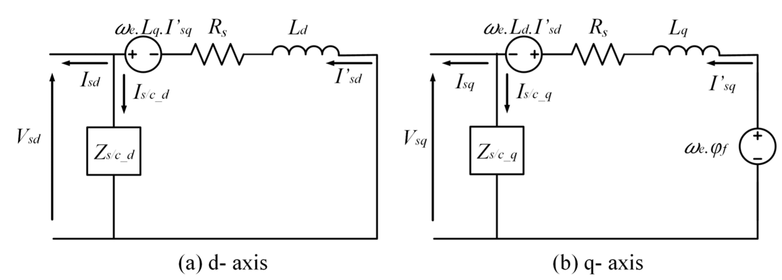
2.2. PMSG Faulty State Model

In the case of a PMSG stator winding fault, the number of turns in a certain phase is reduced due to the deterioration in the stator winding insulation, which causes a short circuit in this phase. Most stator winding insulation failures are caused by high temperatures and overloading. When a stator winding short circuit happens, the value of generator impedance changes, consequently the amplitude of stator current harmonics will increase, the torque will drag, and potential overheating will appear, and so on, this symptom may lead to complete failure if the fault was not addressed.
The short circuit current [ I s / c ]dq is generated inside the machine as shown in Figure 3 due to the presence of the short circuit impedance Z s / c in any phase; this impedance value changes according to the ratio between the number of inter-turn short-circuit windings and the total number of turns in one healthy phase. Figure 4 shows the equivalent circuit of the faulty machine in the dq-frame. The mathematical equations representing the faulty state model of the PMSG in dq-frame are given in [39].

3. Parameter Estimation Procedures

The general faulty PMSG state-space model and EKF algorithm are presented in this section.

3.1. General PMSG State-Space Model

To use the EKF and UKF techniques to estimate the presence of the fault, the precise state-space model of the machine should be highlighted. Based on [39], the state-space model equation of the faulty machine can be written as:
{ x ˙ m ( t ) = A m · x m ( t ) + B m · u m ( t ) + W m ( t ) y m ( t ) = C m · x m ( t ) + D m · u m ( t ) + V m ( t )      
where:
x m ( t ) = [ I s d I s q ] T   u m ( t ) = [ V s d V s q φ f ] T A m = [       R s   L d   ω e · L q L d ω e · L d L q R s   L q ]
B m = [ 1 L d 0 0 0 1 L q ω e L q ]             C m = [       1 0 0 1     ]
D m = [ D 1 0 ] T    D 1 = k = 1 3 2 · n s / c   k ( 3 2 · n s / c   k   ) · R s · P ( θ ) T · Q ( θ s / c     k ) · P ( θ )
where
P ( θ ) = [   c o s θ s i n θ s i n θ c o s θ ]
Q ( θ S / C ) = [     c o s 2 θ S / C s i n θ S / C · c o s θ S / C s i n θ S / C · c o s θ S / C s i n 2 θ S / C     ]
The extension of the model states to estimate the presence of a fault in any phase is compulsory for the estimation process of EKF and UKF, the new states of the model become as follows:
X ˜ e ( t ) = [ X ( t ) λ ( t ) ] = [ I s d I s q n A   s / c   n B   s / c   n C   s / c   ] T
where X ˜ e ( t ) is the estimated state; After that, the model equations are linearized around a definite operating point followed by discretization at a sampling time Ts, the model expressed as:
[ I ˙ s d I ˙ s q n ˙ A   s / c n ˙ B   s / c n ˙ C   s / c ] = [ 1 T s R s L d T s · w e · L q L d 0 0 0 T s · w e · L d L q 1 T s R s L q 0 0 0 0 0 1 0 0 0 0 0 1 0 0 0 0 0 1 ] [ I s d I s q n A   s / c   n B   s / c   n C   s / c   ]   +   [ T s L d 0 0 T s L q     0 ω e L q 0             0 0             0 0             0             0 0 0 ] [ V s d V s q φ f ]

3.2. Extended Kalman Filter Algorithm

The EKF gives an approximation of the optimal estimate. The non-linearity of the system’s dynamics is approximated by a linearized version of the non-linear system model around the last state estimate. As in many cases, if the nonlinear system is approximately linearized, the EKF may not perform well [20]. If there is a bad initial guess regarding the underlying system’s state, then this may cause a bad estimation. The first step in the EKF algorithm is the prediction step equations, which consist of state prediction and error covariance matrix update, and the second step is the correction step which corrects the predicted state estimate and it’s covariance matrix as in Figure 5. Consider applying EKF to estimate the parameter λ k in the PMSG system, the discrete linearized state-space model of PMSG is expressed as:
{       X ˜ e k + 1 = F ˜ k   X ˜ e k + W k Y ˜ k = H ˜ k     X ˜ e k + V k
where
{ F ˜ K = [ 1 + T s A ( λ k ) T s ( A ( λ k λ k X k   +   B ( λ k λ k U k ) 0 I ] H ˜ K = [ C ( λ k )     ( C ( λ k λ k X k   +   D ( λ k λ k U k ) ]
F ˜ K and H ˜ K represent the state and output equations of the discrete linearized model. By substituting matrix A and B in (4) into (6), F ˜ K and H ˜ K in case of, n A   s / c   , n B   s / c   , n C   s / c   ,   as an estimated parameter will be:
F ˜ K = [ 1 T s R s   L d   T s · ω e · L q L d 0 0 0 T s · ω e · L d L q 1 T s R s   L d 0 0 0 0 0 1 0 0 0 0 0 1 0 0 0 0 0 1 ] H ˜ K = [ 1 0 0 1 S A × q 1 S B × q 1 S C × q 1 S A × q 2 S B × q 2 S C × q 2 ]
where
S A = 6 / ( ( 3 2 n A   s / c   ) 2 × R s     )   S B = 6 / ( ( 3 2 n B   s / c   ) 2 × R s   )
S C = 6 / ( ( 3 2 n C   s / c   ) 2 × R s   )         [ q 1 q 2 ] = [ P ( θ ) T · Q ( θ s c   k ) · P ( θ ) ] 2 x 2 · [ V s d V s q ]

3.3. Unscented Kalman Filter Algorithm

Instead of using linearized equations using the Jacobin matrix to approximate the nonlinear model as the EKF approach, the UKF generates a finite set of sigma points to compute the predicted states and measurements and the associated covariance matrices [45]. Mathematically, the UKF process can be described as in Figure 6.
Where W i m and W i c are weighting factors and they are equal to.
W i m = W i C = 1 / 2 ( L + λ )
where L is the state dimension and λ = α 2 ( ( L + k ) L ) , α can be tuned from 10 4 to 1 and k usually was chosen to be 0.
Figure 7 shows the block diagram of the fault diagnosis online monitoring for the PMSG.

3.4. The Covariance Matrices Tuning

The noises covariance matrices are diagonals, Q can be divided into two matrices: q x (for measured states) and q λ (for the estimated parameters). Thus, Q and R can be expressed as:
{ Q = q x · [ I m 0 0 q λ q x · I n ] R = r · I m                                  
where m is the state’s x numbers and n is estimated parameters λ numbers, q x and r could be determined by measuring the variance of noises on input σ u 2   and output signals   σ y 2 [20], they are expressed as Equation (9) and the ratio q λ   / q x   is set by the evolution time constant of the estimated parameters (τ )   as expressed in Equation (10).
{ q x = ( f k u k ) 2 · σ u 2 r =   ( H k X k ) 2 · σ y 2
q λ q x T s τ · i = 1 n ( | f k i u k | · | h k i X k | ) 2

4. Simulation Results

The machine parameters were taken from the nameplate of the generator, as shown in Table 1, the equations of the generator were used to simulate the output of the machine with different operating points, and the simulation run at sampling time T s = 100   us .

4.1. EKF VS. UKF Response

Figure 8 shows the instantaneous internal current of phase A of the machine at RMS load current of 0.75 A and frequency of 30 Hz; a simulated inter-turn fault was implemented at t = 0.5 s, this fault caused an increase in the current inside the machine, respectively, the voltage in the faulty phase decreased by a small amount and the machine started to become hotter. The current reached an RMS value of 1.63 in the case of n A   s / c   = 4%, which is more than double the used load current. Also, the current reached an RMS value of 4.6 A in the case of n A   s / c   = 16%, which is more than 6 times the load current (0.75 A). This implies the importance of taking fast action to save the machine from damage.
Figure 9 shows the estimation response of EKF and UKF in either a healthy or faulty state; it was noticed that the UKF technique gives more precise values for the fault estimation than the EKF. As the PMSG model used is a linearized and discretized model around a specified operating point in the case of EKF, the error in the estimation varies non-linearly with the value of the short circuit turns ratio. Besides, the covariance matrices ( Q and R ) were chosen, which play an important role in the quality of the estimation. Also, the presence of sensor errors and the use of a phased locked loop (PLL) in the estimation of the angular position θ cause error in the estimated parameters. Figure 10 shows the error-index, which indicates the values of the inter-turn short circuit that the EKF and UKF techniques will estimate varies the percentage of error. It was noticed that the UKF had much less error than the EKF, especially for short circuit turns ratios greater than 20%, the highest error detected in case of using UKF was at n A   s / c   = 4 % and reached 0.3%, however, the EKF estimation error reach 23.72% at   n A   s / c   = 100%, the lowest estimation error detected by EKF was at n   s / c   = 16 % .
The dynamic time response of detecting the fault was 0.02 s, which is very fast (approximately equal to 1.5 periodic cycles related to the used frequency). The covariance matrix Q , in this case, was tuned by time constant τ = 5 ms, which increased the dynamic response; however, it increased the presence of noise in the estimation action. Figure 11 illustrates the effect of τ on the estimation time, and it was noticed that when the τ = 10 ms, the estimation response reached a steady-state after 0.02 s with the presence of noise, however, when the τ = 80 ms, the estimation response reached a steady-state after 0.2 s but with filtering action. Figure 12 shows the dynamic estimation responses versus the parameter estimation evolution time constant (τ); the detection time increased linearly with the increase of the τ value.

4.2. Robustness Tests

The technique was tested in different operating conditions and showed a robust response; the same tests are done in cases of practical implementation, and are listed as the following:
Test 1: Variation of load current variation from 0.75 A to 3 A by 0.75 A step at a constant frequency of 30 Hz.
Test 2: Variation of frequency from 20 Hz to 50 Hz, with a 10 Hz step.

4.3. Load Variation Test

Figure 13 shows the estimated internal instantaneous currents in the presence of a 16% stator inter-turn short circuit in phase A in case of load variation from 0.75 to 3 A with a rate of 1 Hz. In the case of a 16% stator inter-turn fault, the current reached an RMS value of 5.3 A when ILoad = 1.5 A, and it reached an RMS value of 6 A when the ILoad = 2.25 A. This confirms the increase of fault severity as load current increases; this form of the fault requires fast action.
Figure 14 and Figure 15 show the estimation response of EKF and UKF in load current variation from ILoad = 0.75 A to 3 A condition in the presence of 4%, 8%, 12%, and 16% stator inter-turn short circuit by a rate of 1 Hz. The time constant of the estimated parameters (τ) was chosen to be 10 ms based on the measured value of the input signal noises variance (όx). The estimation for both techniques show a constant response with the load variation with different short circuit values.

4.4. Frequency Variation Test

Figure 16 shows the estimated internal instantaneous currents in the case of faults in various frequencies, ranging from 20 Hz to 50 Hz with 10Hz step frequency and rate of change of 1 Hz. Figure 17 and Figure 18 show the EKF the UKF estimation response in the presence of 4%, 8%, 12%, and 16% stator inter-turn short circuit in phase A at constant ILoad = 0.75 A and frequencies of 20 Hz, 30 Hz, 40 Hz and 50 Hz. The results show a constant response for both techniques with the frequency variation condition.

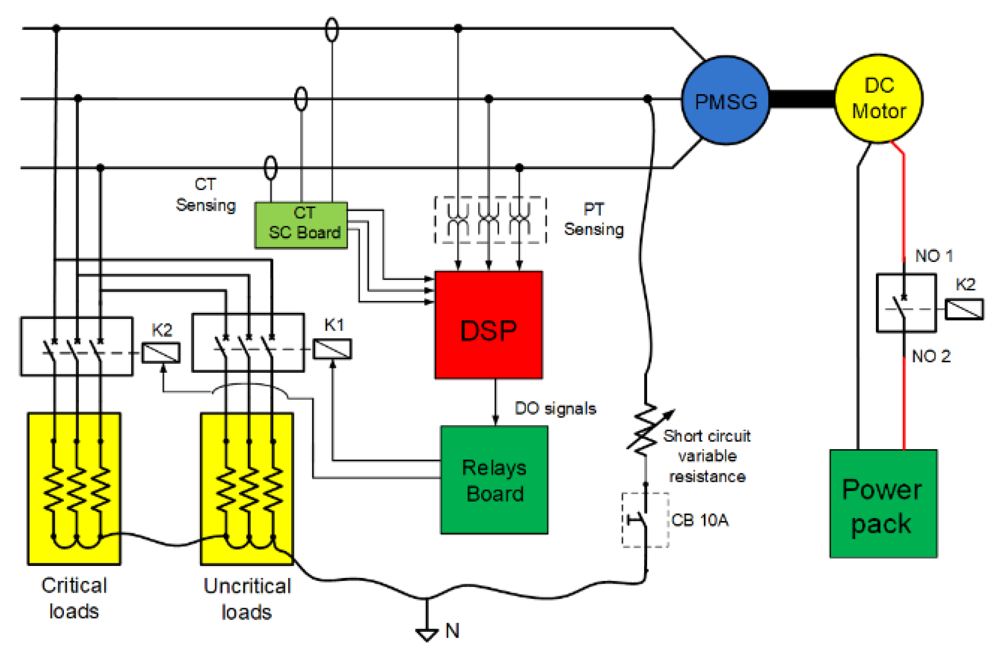
5. Experimental Results

5.1. Test Bench

For safety conditions, to prevent the used PMSG from being damaged, it is not possible to make an actual stator inter-turn fault. However, it is possible to validate this detection method by adding a shunt resistance R S / C between the needed phase and the neutral, to increase the current in this phase and make the machine unbalanced by a percentage equal to that of an inter-turn fault.
The generator used rotates by means of a separately excited DC motor as a prime mover; the shaft of the motor is coupled directly to the shaft of the PMSG. The power pack supplies the DC motor field with a constant DC supply, and the armature is supplied with a variable DC supply to control the speed of the generator. The load used is a three-phase variable load with a maximum RMS value of 5 A; the shunt resistance R S / C is variable resistance, which will be added to any phase of the three phases using a circuit breaker. Figure 19 shows all the power components of the test bench.
The three-phase voltages were measured by three voltage transformers. The transformers used were typical 220 v/12 v single-phase transformers. Hence, the voltages measured were connected to analog signal conditioning boards to manipulate the voltage to be level with the digital signal processor (DSP) voltage (from 0 to 3.3 v).
On the other hand, the currents were measured using three CTs at a ratio of 10000:5. The current signals measured were connected to the signal conditioning circuit board to convert the current into a manipulated voltage which was compatible with a DSP analog to digital (A/D) input. The DSP used (Texas Instrument TMS320F280) had all measured signals connected to the A/D port in the DSP. The EKF algorithm was implemented online with a sampling period of T s = 200 μs. The relay board was used to take the action of disconnection of the faulty phase to prevent fault propagation leading to severe failure. Figure 20 shows the connection diagram for the whole circuit.

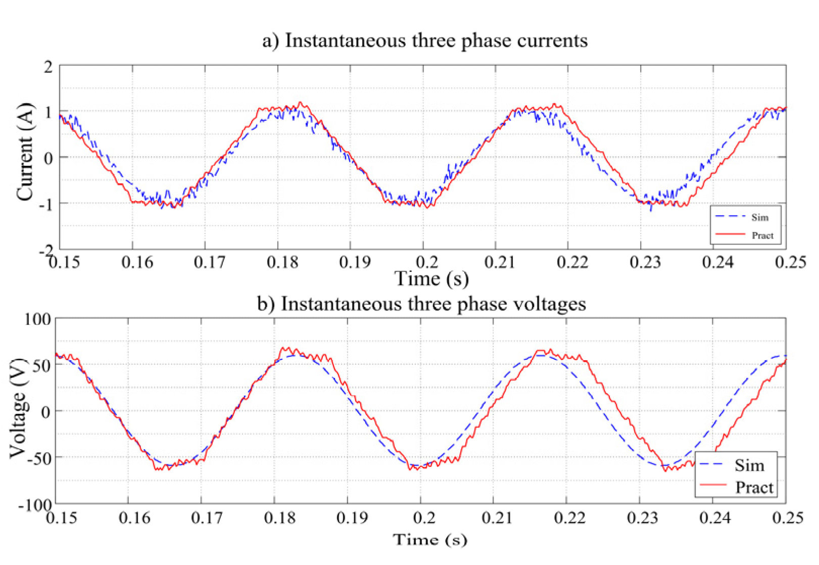
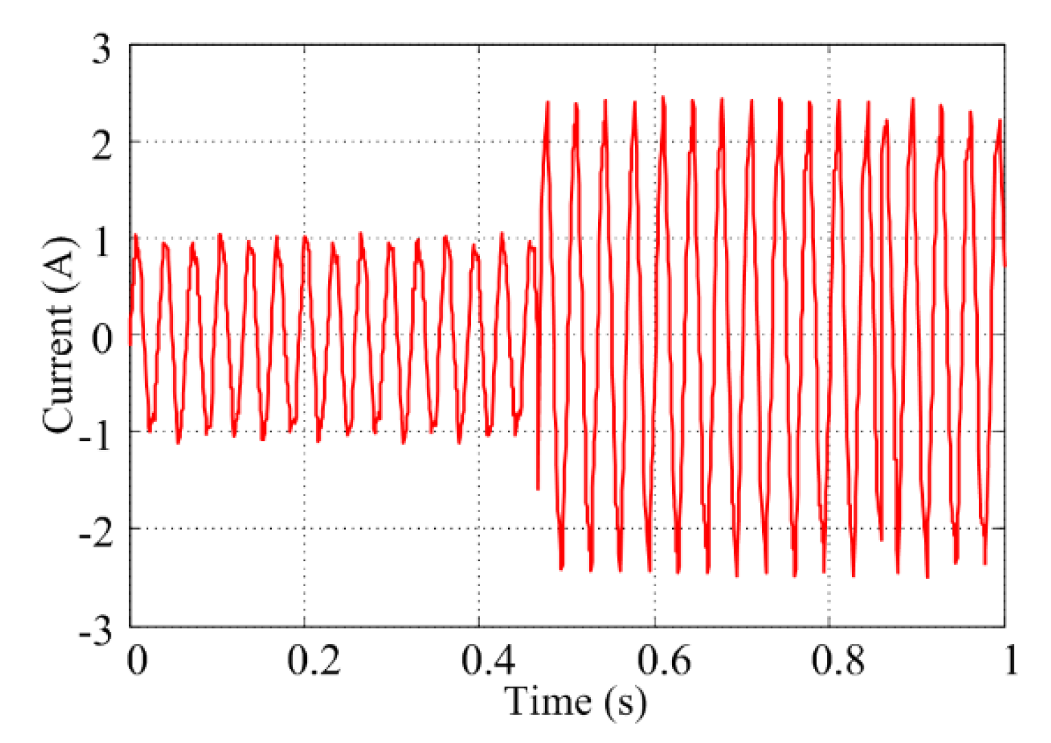
5.2. PMSG Test Output
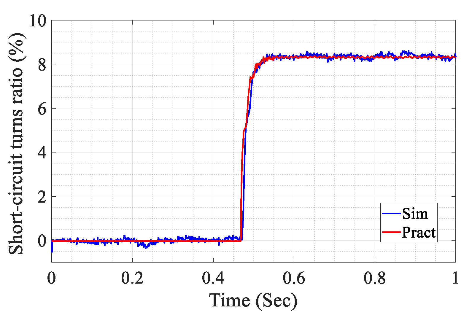
The next step was to compare the measured output voltages and currents of the PMSG used in a simulation of a healthy state. The value of the measured currents and voltages was found to be approximately the same as that in simulation, but with more measurement noise around a mean of 0.4; this will affect the dynamic response of EKF estimation in case of a fault. The output was measured in different load and frequency operating conditions and showed the same output as the simulation. Figure 21a,b show the instantaneous three-phase currents and voltages in the case of a healthy state of PMSG with a load current 0.72 A and frequency of 30 Hz.
Figure 22 shows the difference between the three-phase instantaneous currents and voltages in simulation and practical implementations. It can be seen that the experimental results appear noisier than that of the simulation. Accordingly, the parameter estimation responses will require more filtering action, which will cause a delay in the dynamic response.

5.3. EKF Response

The model of a faulty machine and the EKF model were implemented in the DSP, the input to the machine state-space model are the measured stator voltages in the dq-frame. The short circuit current was calculated from the measured dq stator load currents and is presented in the model as the feed-forward matrix D m . Therefore, the measured three-phase voltages and currents must be converted in dq-frame to make the EKF estimator work probably.
Indeed, the detection of electrical angular position θ is essential to use it in the abc to dq0 transformation. There are two suitable solutions for the detection of electrical angular position θ ; the first is to use an encoder sensor coupled directly to the machine shaft and uses its counts to calculate the mechanical angular position, and then calculates the electrical angular position. Nevertheless, this solution requires the addition of new hardware to the system. The second solution is to generate the electrical angular position θ from voltage signals through the three phases of the phased locked loop (PLL), this solution is more economical as extra sensing devices are not needed. Nevertheless, the angular position generated will be dependent on the nature of the measured voltage.
The machine works at a load current of 0.72 and a frequency of 30 Hz in a healthy state. The practical experiments tested the EKF estimation responses in different values of short circuit inter-turn to turn the ratio in all phases ( n A   s / c , n B   s / c & n C   s / c ) and in different operating points. The Q and R were tuned at τ = 20 ms to achieve the required fast response with a good filtering action.
Figure 23 display the response of EKF to estimate n A   s / c = 4 %   using these conditions. The parameter estimation showed an excellent response to this case when compared to the results of the simulation. Figure 24 display the estimated internal instantaneous currents in the presence of 4%, stator inter-turn short circuit in phase A at t = 0.5 s, respectively. The same response was noticed on the estimation of n A   s / c = 8 % in Figure 25 followed by the estimated internal instantaneous currents in phase A in Figure 26, respectively. Also, The same response was noticed on the estimation of n A   s / c = 12 % in Figure 27 followed by the estimated internal instantaneous currents in phase A in Figure 28, respectively. In addition, the estimation of the fault in n A   s / c = 16 % casein Figure 29 and it’s etimated internal current in Figure 30. It was noted that the current reached higher values when compared to the rated current of 0.72 A.

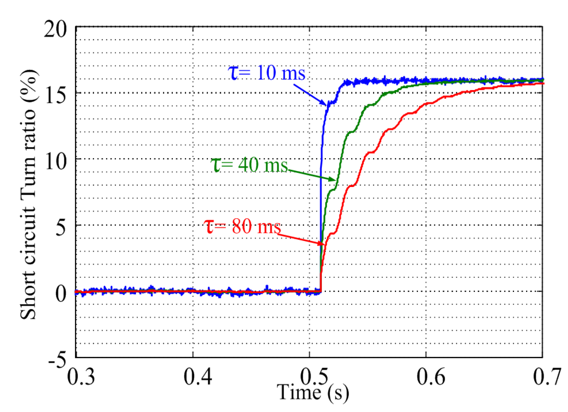
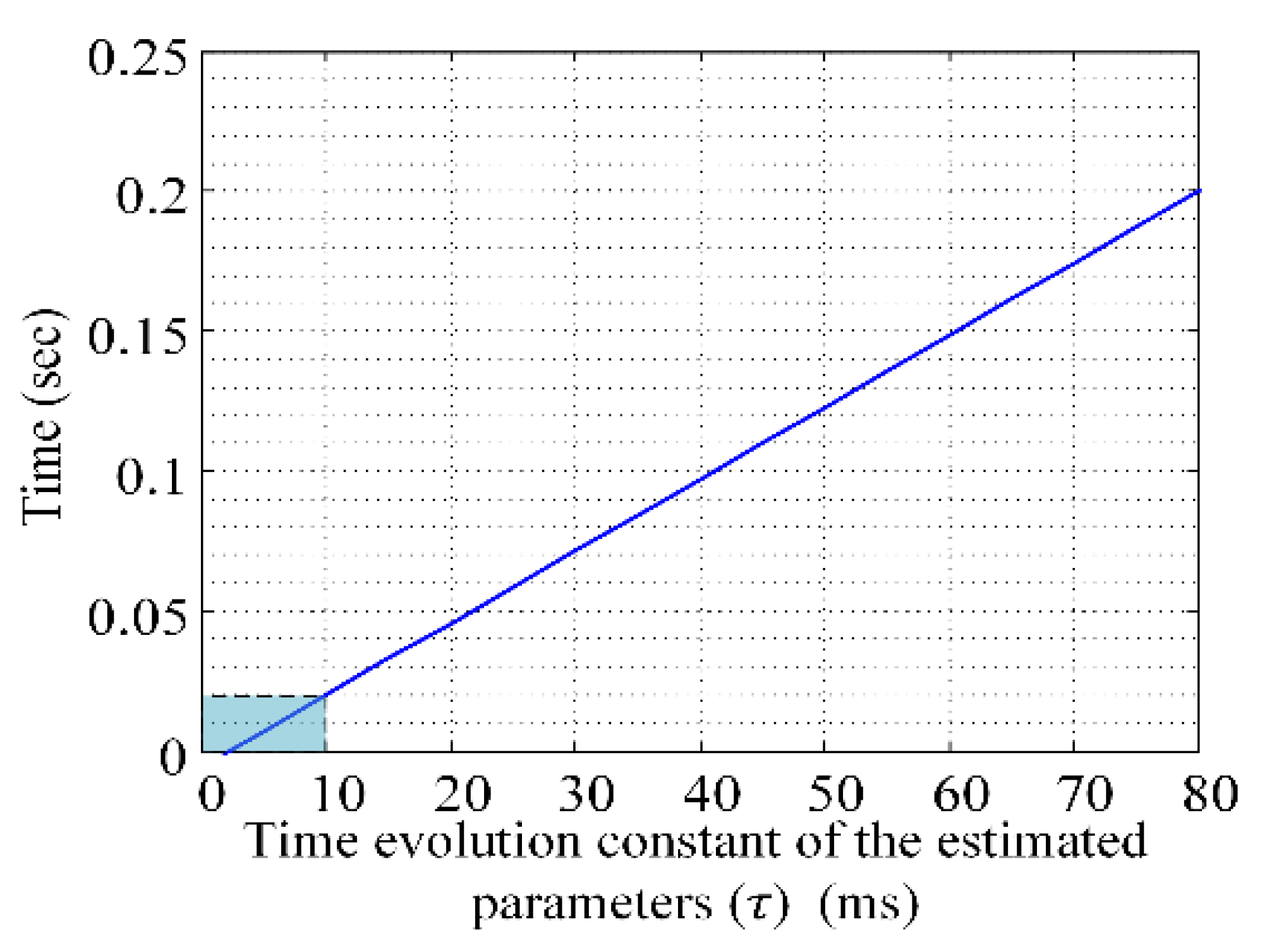
5.4. Tuning of Covariance Matrices

Figure 31 shows the dynamic estimation response with different values of evolution time constant of the estimated parameter (τ) in the presence of a 16% fault in phase A. The weighting matrices ( Q and R ) were chosen based on measuring the variance of input noise and the variance of output noise to achieve the required fast dynamic response for the estimation of the parameters at different operating conditions. However, the change in the weighting matrices caused changes in the nature of the estimation response.

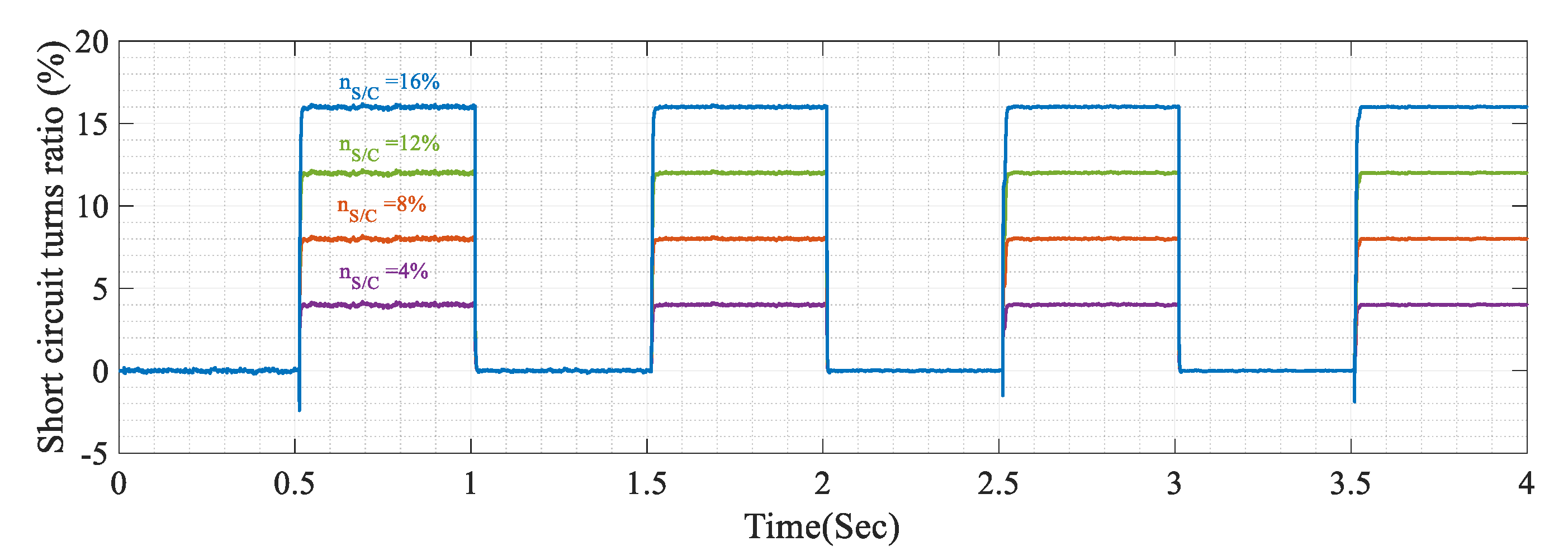
5.5. Robustness Test

As in the simulation, the machine was tested using different load conditions; this approach tested the parameter estimation response to various load conditions. The tests are listed as following:
Test 1: Variation of frequency from 20 Hz to 50 Hz with a 10 Hz step.
Test 2: Variation of load Current variation from 0.72 A to 2.25 A by 0.75 A step at a constant frequency of 30 Hz.
The EKF showed a constant response in assays with different frequencies (20 Hz, 30 Hz, 40 Hz and 50 Hz) in the presence of 4%, 8%, 12%, and 16% stator inter-turn fault in phase A, and a load current of 0.72 A in a healthy state (Table 2). This emphasized the robustness of this technique when there was a variation in frequency. Moreover, the results confirmed the simulation results for the same machine during the same operating and fault conditions.
Besides, the estimation response was tested when exposed to variations in the current (1.5 A and 2.25 A) and at a constant frequency of 30 Hz. Again, the response of the EKF technique showed a robust estimation in load current variation at a constant frequency, (Table 3). For safety conditions, it was not able to emulate short circuit inter turns fault more than 12% as the current in the faulty state went over 5 A; 5 A being the maximum load current for this machine.

5.6. Decision-Making Process

The decision was taken based on the estimated total internal current in all three phases of the machine. The loads were divided into two groups: critical loads and uncritical loads were connected through contactors K2 and K1, respectively. To prevent the propagation of internal inter-turn faults inside the machine, there are two proposed scenarios:
  • the disconnection of the machine;
  • load shedding.
Figure 32 shows the flowchart presenting the FDS EKF technique and the proposed scenarios based on the operator’s choice.

5.6.1. Scenario 1: The Disconnection of the Machine

This solution provides for the safety of the machine and prevents the propagation of the fault to other turns and phases. However, this solution affects the reliability of the operation, and it requires a backup for the disconnected generator.
This scenario is presented in the experimental work at RMS load current of 1.5 and 30 Hz frequency, in a healthy state the machine gives n A   s / c   = 0,   n B   s / c   = 0 and n C   s / c   = 0. At t = 0.5 s. A 4% inter-turn fault exists in phase A, the estimated parameter n A   s / c = 4.1% and the total estimated internal current reached an RMS value of 2.8 A. As the FDS works in parallel with the protection system of the machine, the disconnection of the machine will be based on the extremely inverse time (EIT) thermal characteristics curve of overcurrent relay based on IEEE standard [46], the expected time to disconnect the machine is 17 s, at TDS = 0.1 s. Figure 33b,c show the detection time and disconnection time of contactor K1 and contactor K2 after detecting the presence of a fault. An LCD was used to monitor the situation of the machine in both the healthy and faulty states; it also shows the expected disconnection time of both contactors and the position of the loads’ contactor to inform the operator about the situation.

5.6.2. Scenario 2: Load Shedding

The second scenario is the disconnecting of some uncritical loads (contactor K1) to decrease the total current of the machine allowing it to run under the fault condition. This solution offers the reliability for the process; the machine can continue running in the presence of a fault but with partial loading. This solution does not solve the main problem of internal fault, but it gives the operator a suitable time to take corrective action; the fault may propagate for other turns or phases, respectively, increasing the internal short circuit current, causing a severe fault.
This scenario was implemented at RMS load current of 1.5 A and 30 Hz frequency; at t = 0.5 s, 2% inter-turn fault was emulated in phase C, which caused an increase in the total estimated internal current to 2 A. The fault was indicated, and the first group of loads (the uncritical loads) connected through contactor K1 was disconnected (Figure 34a). The disconnection of K1 decreased the current in the machine, and the total current became 1.25 A, allowing the machine to return to its normal state for a definite time and consequently canceling the alarm indication. After a time, the fault percentage increased to 8%, causing an increase in the internal current. In this case, the right decision was to disconnect the machine to solve the internal fault problem. The machine was disconnected after the estimated time based on the EIT characteristics of the overcurrent relay.

6. Conclusions

The paper presents the detection and isolation of PMSG stator windings faults using the EKF and the UKF, which are model-based techniques. The model of the faulty machine was implemented in the state-space model using the machine equations in the dq-frame. The estimated states of the EKF and the UKF techniques were the short circuit turns ratio in each phase. It was noted that the proposed techniques have the following advantages:
  • a fast and accurate response in relation to the time needed to take action in real time;
  • a robust estimation, in the presence of process and measurement noises, in addition to load and frequency variations.
On the other hand, the UKF technique overcomes the EKF technique drawback of the inaccuracy of the technique in case of severe faults, as it is a nonlinear system and it was linearized around a definite operating point, and so the error of estimation increased as the value of the short circuit turn ratio increased.
Also, the tuning of the weighting matrices ( Q and R ) has a great impact on the estimated parameters. As indicated in the result, an increase in Q implies an acceleration of the dynamic response of the fault indicator with an increase in noise sensitivity, however, decreasing Q implies better filtering with a decrease in the dynamic response.
The results of this paper point to several exciting directions for future research work. The proposed technique can be used on FD of different types of faults such as bearing, eccentricity, and demagnetizations faults in machines. Moreover, other types of FD techniques may be used, such as artificial intelligence-based techniques and signal-based techniques, and comparing their results with the results of the EKF Technique. This result raises the ability to implement the fault tolerant control (FTC) technique in case of faults such as using the model predictive control (MPC) [47], which would increase the reliability of the machine safety-critical applications.

Author Contributions

Conceptualization, W.E.S., M.A.E.G. and A.L.; methodology, W.E.S. and M.A.E.G.; software, W.E.S.; validation, W.E.S., M.A.E.G. and A.L.; formal analysis, W.E.S., M.A.E.G. and A.L.; investigation, W.E.S., M.A.E.G. and A.L.; resources, W.E.S. and M.A.E.G.; data curation, W.E.S. and M.A.E.G.; writing—original draft preparation, W.E.S. and M.A.E.G.; writing—review and editing, W.E.S. and M.A.E.G.; visualization, W.E.S.; supervision, M.A.E.G. and A.L.; All authors have read and agreed to the published version of the manuscript.

Funding

This research received no external funding.

Conflicts of Interest

The authors declare no conflict of interest.

Nomenclature

L d Direct stator synchronous inductance.mH y m ( t ) Output vector.
L q Quadrature stator synchronous inductance.mH T s Sampling period.Sec
[ V s ] d q Direct and quadrature stator voltages.Volts I S / C Short-circuit current.Ampere
P ( θ ) dq transformation matrix. R S / C Short-circuit resistance.Ω
θ Electrical angular position.rad n S / C Short-circuited turns ratio.%
ω e Electrical angular velocityrad/s F ˜ k State equation of the discrete model.
[E]Electromotive forces vector.Volt A m State matrix.
[ Z s / c   ] Equivalent fault impedance.Ω Q State noises covariance matrix.
X ˜ e k Extended state vector. W m ( t ) State noises vector.
X ^ k | k Extended state vector. x m ( t ) State vector.
θ s c   Fault localization angle. [ I s ] d q Stator currents vector after variable change in dq-frame.Ampere
Q ( θ s c   k ) Fault localization matrix. [ I s ] d q Stator currents vector in dq-frame.Ampere
D m Feed forward matrix. R S Stator resistance.Ω
JInertiaKg.m2 L S Stator synchronous inductance.mH
B m Input matrix. PThe electromechanical powerWatts
u m ( t ) Input vector.- P k | k The error covariance matrix at time k
K k Kalman gain H ˜ k The output equations of the discrete linearized model.
T m Load torqueNm P k | k 1 The prior estimate of   P k  
R Measurement noises covariance matrix F ˜ K The state equations of the discrete linearized model.
V m ( t ) Measurement noises vector. τThe time constant of the estimated parameters.Sec
H k Output equation of the discrete model. σ u The variance of input signals noises.
C m Output matrix. σ y The variance of output signals noises.

References

  1. Zhang, Y.; Ji, T.Y.; Li, M.S.; Wu, Q.H.; Wu, Q.H. Application of Discrete Wavelet Transform for Identification of Induction Motor Stator Inter-turn Short Circuit. In Proceedings of the 2015 IEEE Innovative Smart Grid Technologies—Asia, ISGT ASIA 2015, Bangkok, Thailand, 3–6 November 2016. no. 51207058. [Google Scholar]
  2. Wang, H.; Yang, J.; Chen, Z.; Ge, W.; Ma, Y.; Xing, Z.; Yang, L. Model Predictive Control of PMSG—Based Wind Turbines for Frequency Regulation in an Isolated Grid. IEEE Trans. Ind. Appl. 2018, 54, 3077–3089. [Google Scholar] [CrossRef]
  3. Fakhari, M.; Arani, M. Assessment and Enhancement of a Full-Scale PMSG-Based Wind Power Generator Performance Under Faults. IEEE Trans. Energy Convers. 2016, 31, 728–739. [Google Scholar]
  4. Jiang, Y.; Zhang, Z.; Jiang, W.; Geng, W.; Huang, J. Three-phase current injection method for mitigating turn-to-turn short-circuit fault in concentrated-winding permanent magnet aircraft starter generator. IET Electr. Power Appl. 2018, 12, 566–574. [Google Scholar] [CrossRef]
  5. Gao, F.; Zheng, X.; Bozhko, S.; Hill, C.I.; Asher, G. Modal Analysis of a PMSG-Based DC Electrical Power System in the More Electric Aircraft Using Eigenvalues Sensitivity. IEEE Trans. Transp. Electrif. 2015, 1, 65–76. [Google Scholar]
  6. Sarigiannidis, A.; Kladas, A. High Efficiency Shaft Generator Drive System Design for Ro-Ro Trailer-passenger Ship Application. In Proceedings of the 2015 International Conference on Electrical Systems for Aircraft, Railway, Aachen, Germany, 3–5 March 2015. Ship Propulsion and Road Vehicles (ESARS). [Google Scholar]
  7. Wang, Z.; Yang, J.; Ye, H.; Zhou, W. A Review of Permanent Magnet Synchronous Motor Fault Diagnosis. In Proceedings of the 2014 IEEE Conference and Expo. Transportation Electrification Asia-Pacific (ITEC Asia-Pacific), Beijing, China, 31 August–3 September 2014; pp. 1–5. [Google Scholar]
  8. Ebrahimi, B.M.; Roshtkhari, M.J.; Faiz, J.; Khatami, S.V. Advanced eccentricity fault recognition in permanent magnet synchronous motors using stator current signature analysis. IEEE Trans. Ind. Electron. 2014, 61, 2041–2052. [Google Scholar] [CrossRef]
  9. Rosero, J.; Romeral, L.; Rosero, E.; Urresty, J. Fault Detection in dynamic conditions by means of Discrete Wavelet Decomposition for PMSM running under Bearing Damage. In Proceedings of the 2009 Twenty-Fourth Annual IEEE Applied Power Electronics Conference and Exposition, Washington, DC, USA, 15–19 Febuary 2009; pp. 951–956. [Google Scholar]
  10. Ebrahimi, B.M.; Faiz, J.; Roshtkhari, M.J. Static-, dynamic-, and mixed-eccentricity fault diagnoses in permanent-magnet synchronous motors. IEEE Trans. Ind. Electron. 2009, 56, 4727–4739. [Google Scholar] [CrossRef]
  11. Pacas, M.; Villwock, S.; Dietrich, R. Bearing Damage Detection in Permanent Magnet Synchronous Machines. In Proceedings of the 2009 IEEE Energy Conversion Congress and Exposition, San Jose, CA, USA, 20–24 September 2009; pp. 1098–1103. [Google Scholar]
  12. Soualhi, A.; Jean-monnet, U.; Lyon, U. Early Detection of Bearing Faults by the Hilbert-Huang Transform. In Proceedings of the 2016 4th International Conference on Control. Engineering & Information Technology (CEIT-2016), Hammamet, Tunisia, 16–18 December 2016; pp. 16–18. [Google Scholar]
  13. Rosero, J.; Romeral, J.L.; Cusido, J.; Ortega, J.A.; Garcia, A. Fault Detection of Eccentricity and Bearing Damage in a PMSM by Means of Wavelet Transforms Decomposition of the Stator Current. In Proceedings of the 2008 Twenty-Third Annual IEEE Applied Power Electronics Conference and Exposition, Austin, TX, USA, 24–28 Febuary 2008; pp. 111–116. [Google Scholar]
  14. Huang, T.; Fu, S.; Feng, H.; Kuang, J. Bearing Fault Diagnosis Based on Shallow Multi-Scale Convolutional Neural Network with Attention. Energies 2019, 12, 3937. [Google Scholar] [CrossRef] [Green Version]
  15. Zhang, H.; Zhang, S.; Yin, Y. A Novel Improved ELM Algorithm for a Real. Math. Probl. Eng. 2014, 2014. [Google Scholar] [CrossRef]
  16. Vinson, G.; Combacau, M.; Prado, T.; Ribot, P. Permanent Magnets Synchronous Machines Faults Detection and Identification. In Proceedings of the IECON 2012—38th Annual Conference on IEEE Industrial Electronics Society, Montreal, QC, Canada, 25–28 October 2012; pp. 3925–3930. [Google Scholar]
  17. Espinosa, A.G.; Rosero, J.A.; Cusidó, J.; Romeral, L.; Ortega, J.A. Fault detection by means of Hilbert-Huang transform of the stator current in a PMSM with demagnetization. IEEE Trans. Energy Convers. 2010, 25, 312–318. [Google Scholar] [CrossRef] [Green Version]
  18. Ruiz, J.R.R.; Rosero, J.A.; Espinosa, A.G.; Romeral, L. Detection of demagnetization faults in permanent-Magnet synchronous motors under nonstationary conditions. IEEE Trans. Magn. 2009, 45, 2961–2969. [Google Scholar] [CrossRef]
  19. Obeid, N.H.; Boileau, T.; Nahid-Mobarakeh, B. Modeling and diagnostic of incipient interturn faults for a three-phase permanent magnet synchronous motor. IEEE Trans. Ind. Appl. 2016, 52, 4426–4434. [Google Scholar] [CrossRef]
  20. Aubert, B.; Regnier, J.; Caux, S.; Alejo, D. Kalman-Filter-Based Indicator for Online Interturn Short Circuits Detection in Permanent-Magnet Synchronous Generators. Ind. Electron. IEEE Trans. 2015, 62, 1921–1930. [Google Scholar] [CrossRef]
  21. Chen, Y.; Liang, S.; Li, W.; Liang, H.; Wang, C. Faults and Diagnosis Methods of Permanent Magnet Synchronous Motors: A Review. Appl. Sci. 2019, 9, 2116. [Google Scholar] [CrossRef] [Green Version]
  22. Liang, H.; Chen, Y.; Liang, S.; Wang, C. Fault Detection of Stator Inter-Turn Short-Circuit in PMSM on Stator Current and Vibration Signal. Appl. Sci. 2018, 8, 1677. [Google Scholar] [CrossRef] [Green Version]
  23. Kościelny, J.M.; Syfert, M.; Sztyber, A. Advanced Solutions in Diagnostics and Fault Tolerant Control; Springer: New York, NY, USA, 2017. [Google Scholar]
  24. Duque-Perez, O.; del Pozo-Gallego, C.; Morinigo-Sotelo, D.; Godoy, W.F. Condition monitoring of bearing faults using the stator current and shrinkage methods. Energies 2019, 12, 3392. [Google Scholar] [CrossRef] [Green Version]
  25. Helal, A.H.; Badran, E.F.; Ashour, H.A. Synchronous Generator Stator Earth fault Classification and Location Using Wavelet Transform and ANFIS. In Proceedings of the 2017 Nineteenth International Middle East. Power Systems Conference (MEPCON), Menoufia University, Cairo, Egypt, 19–21 December 2017; pp. 19–21. [Google Scholar]
  26. Devi, N.R. Diagnosis and Classification of Stator Winding Insulation Faults on a Three-phase Induction Motor using Wavelet and MNN. IEEE Trans. Dielectr. Electr. Insul. 2016, 23. [Google Scholar] [CrossRef]
  27. Rosero, J.A.; Romeral, L.; Ortega, J.A.; Rosero, E. Short-circuit detection by means of empirical mode decomposition and Wigner-Ville distribution for PMSM running under dynamic condition. IEEE Trans. Ind. Electron. 2009, 56, 4534–4547. [Google Scholar] [CrossRef]
  28. Cempel, C. Descriptive parameters and contradictions in TRIZ methodology for vibration condition monitoring of machines. Diagnostyka 2014, 15, 51–59. [Google Scholar]
  29. Cempel, C. Generalized singular value decomposition in multidimensional condition monitoring of machines-A proposal of comparative diagnostics. Mech. Syst. Signal. Process. 2009, 23, 701–711. [Google Scholar] [CrossRef]
  30. Patan, K.; Witczak, M.; Korbicz, J. Towards robustness in neural network based fault diagnosis. Int. J. Appl. Math. Comput. Sci. 2008, 18, 443–454. [Google Scholar] [CrossRef] [Green Version]
  31. Skowron, M.; Orlowska-Kowalska, T.; Wolkiewicz, M.; Kowalski, C.T. Convolutional neural network-based stator current data-driven incipient stator fault diagnosis of inverter-fed induction motor. Energies 2020, 13, 1475. [Google Scholar] [CrossRef] [Green Version]
  32. Medoued, A.; Lebaroud, A.; Laifa, A.; Sayad, D. Feature form Extraction and Optimization of Induction Machine Faults Using PSO Technique. In Proceedings of the 3rd International Conference on Electric Power and Energy Conversion Systems, Istanbul, Turkey, 2–4 October 2013; pp. 1–5. [Google Scholar]
  33. Quiroga, J.; Liu, L.; Cartes, D.A. Fuzzy Logic Based Fault Detection of PMSM Stator Winding Short under Load Fluctuation Using Negative Sequence Analysis. In Proceedings of the American Control, Seattle, WA, USA, 11–13 June 2008; pp. 4262–4267. [Google Scholar]
  34. Mini, V.P.; Sivakotaiah, S.; Ushakumari, S. Fault Detection and Diagnosis of an Induction Motor Using Fuzzy Logic. In Proceedings of the IEEE Region 8 SIBIRCON-2010, Irkutsk Listvyanka, Russia, 11–15 July 2010; pp. 459–464. [Google Scholar]
  35. Korbicz, J.; Kowal, M. Neuro-fuzzy networks and their application to fault detection of dynamical systems. Eng. Appl. Artif. Intell. 2007, 20, 609–617. [Google Scholar] [CrossRef]
  36. Pazera, M.; Korbicz, J. A Process Fault Estimation Strategy for Non-linear Dynamic Systems Marcin. In Proceedings of the International Conference on Recent Trends in Physics (ICRTP 2016), Lille, France, 17–18 November 2016; Volume 755. [Google Scholar]
  37. Pazera, M.; Witczak, M.; Korbicz, J. Combined Estimation of Actuator and Sensor Faults for Non-linear Dynamic Systems. In Proceedings of the 2017 22nd International Conference on Methods and Models in Automation and Robotics, Miedzyzdroje, Poland, 28–31 August 2017; pp. 933–938. [Google Scholar]
  38. Khov, M.; Regnier, J.; Faucher, J. Monitoring of Turn Short-circuit Faults in Stator of PMSM in Closed Loop by On-line Parameter Estimation. In Proceedings of the 2009 IEEE Int. Symp. Diagnostics Electr. Mach. Power Electron. Drives, Cargese, France, 31 August–3 September 2009. [Google Scholar]
  39. Wafik, W.; El-geliel, M.A.; Lotfy, A. PMSG Fault Diagnosis in Marine Application. In Proceedings of the 2016 20th International Conference on System Theory, Control. and Computing (ICSTCC), Sinaia, Romania, 13–15 October 2016; pp. 626–631. [Google Scholar]
  40. Saad, W.W.; El-geliel, M.A.; Lotfy, A. IM Stator Winding Faults Siagnosis Using EKF. In Proceedings of the 2017 fifth Advanced Control Circuits and Systems (ACCS’017), Alexandria, Egypt, 5–8 November 2017; pp. 34–39. [Google Scholar]
  41. Lončarek, T.; Lešić, V.; Vašak, M. Increasing Accuracy of Kalman Filter-based Sensorless Control of Wind Turbine PM Synchronous Generator. In Proceedings of the 2015 IEEE International Conference on Industrial Technology (ICIT), Seville, Spain, 17–19 March 2015; pp. 745–750. [Google Scholar]
  42. Zawirski, K.; Janiszewski, D.; Muszynski, R. Unscented and extended Kalman filters study for sensorless control of PM synchronous motors with load torque estimation. Bull. POLISH Acad. Sci. Tech. Sci. 2013, 61, 793–801. [Google Scholar] [CrossRef]
  43. Kościelny, J.M.; Syfert, M.; Tabor, Ł. Application of Knowledge AboutResidual Dynamics for Fault Isolation and Identification. In Proceedings of the Conference on Control. and Fault-Tolerant Systems, SysTol, Nice, France, 9–11 October 2013; pp. 275–280. [Google Scholar]
  44. Sztyber, A.; Ostasz, A.; Koscielny, J.M. Graph of a process—A new tool for finding model structures in a model-based diagnosis. IEEE Trans. Syst. Man, Cybern. Syst. 2015, 45, 1004–1017. [Google Scholar] [CrossRef]
  45. Wan, E.A.; van der Merwe, R. The Unscented Kalman Filter for Nonlinear Estimation. In Proceedings of the IEEE 2000 Adaptive Systems for Signal. Processing, Communications, and Control. Symposium (Cat. No.00EX373), Lake Louise, AB, Canada, 4 October 2002; pp. 153–158. [Google Scholar]
  46. Electric, S. Extremely Inverse Time (EIT) Curves Current I / I s; Schneider Electric: Rueil-Malmaison, France, 2008; p. 3000. [Google Scholar]
  47. Witczak, P.; Luzar, M.; Witczak, M.; Korbicz, J. A Robust Fault-tolerant Model Predictive Control for Linear Parameter-varying Systems. In Proceedings of the 2014 19th International Conference on Methods and Models in Automation and Robotics (MMAR), Miedzyzdroje, Poland, 2–5 September 2014; pp. 462–467. [Google Scholar]
Figure 1. The equivalent circuit of healthy permeant magnet synchronous generator (PMSG) in the abc-frame.
Energies 13 02972 g001
Figure 2. The equivalent circuit of healthy PMSG in the dq-frame.
Energies 13 02972 g002
Figure 3. The short circuit turns ratio representation.
Energies 13 02972 g003
Figure 4. The equivalent circuit of the faulty state PMSG in the dq-frame.
Energies 13 02972 g004
Figure 5. Extended Kalman filter (EKF) algorithm equations.
Energies 13 02972 g005
Figure 6. Unscented Kalman filter (UKF) algorithm equations.
Energies 13 02972 g006
Figure 7. PMSG fault diagnosis on-line monitoring block diagram.
Energies 13 02972 g007
Figure 8. The instantaneous currents of phase A in case of inter-turn fault at 0.72 A load and 30 Hz frequency.
Energies 13 02972 g008
Figure 9. EKF estimation response in phase A at a load of 0.72 A and a frequency of 30 Hz.
Energies 13 02972 g009
Figure 10. Error Index of the estimated parameter n s / c .
Energies 13 02972 g010
Figure 11. Estimation of 16% short circuit turn ratio in phase B in case of different τ.
Energies 13 02972 g011
Figure 12. Index of the estimated parameters n s / c .
Energies 13 02972 g012
Figure 13. The instantaneous currents of phase A in case of fault at constant frequency of 30 Hz and current variation from 0.75 A to 3 A with step of 0.75 A.
Energies 13 02972 g013
Figure 14. Estimation response in phase A at a frequency of 50 Hz with load variation from 0.75 to 3 A and 7.5 A step.
Energies 13 02972 g014
Figure 15. Estimation response in phase A at a frequency of 50 Hz with load variation from 0.75 to 3 A and 7.5 A step.
Energies 13 02972 g015
Figure 16. The instantaneous currents of phase A in case of fault at 0.75 A load and 50 Hz frequency.
Energies 13 02972 g016
Figure 17. Estimation response in phase A at a load of 0.75 A with frequency variation from 20 to 50 Hz and 10 Hz step.
Energies 13 02972 g017
Figure 18. Estimation response in phase A at a load of 0.75 A with frequency variation from 20 to 50 Hz and 10 Hz step.
Energies 13 02972 g018
Figure 19. Test bench.
Energies 13 02972 g019
Figure 20. Connection diagram.
Energies 13 02972 g020
Figure 21. Instantaneous 3phase currents and voltages.
Energies 13 02972 g021
Figure 22. Simulation vs. Practical implementation 3phase currents and voltages.
Energies 13 02972 g022
Figure 23. Current in phase A at n A   s / c   =   4 % .
Energies 13 02972 g023
Figure 24. Estimation of 4% short circuit turns ratio in phase A.
Energies 13 02972 g024
Figure 25. Current in phase A at n A   s / c   =   8 % .
Energies 13 02972 g025
Figure 26. Estimation of 8% short circuit turns ratio in phase A.
Energies 13 02972 g026
Figure 27. Current in phase A at n A   s / c   =   12 % .
Energies 13 02972 g027
Figure 28. Estimation of 12% short circuit turns ratio in phase A.
Energies 13 02972 g028
Figure 29. Current in phase A at n A   s / c   =   16 % .
Energies 13 02972 g029
Figure 30. Estimation of 16% short circuit turns ratio in phase A.
Energies 13 02972 g030
Figure 31. Estimation response with different τ at a constant frequency of 30 Hz.
Energies 13 02972 g031
Figure 32. Decision-making process scenarios flowchart.
Energies 13 02972 g032
Figure 33. Scenario 1 Alarm indication and machine disconnection.
Energies 13 02972 g033
Figure 34. Scenario 2 Alarm indication and contactors disconnection.
Energies 13 02972 g034
Table 1. The PMSG parameters used.
ParameterSymbolValue
Nominal PowerP1500 W
Nominal current I s   5 A
Nominal Voltage V s   100 v
Nominal Frequencyf50 Hz
Stator resistance R s   1.2 Ω
Direct axis magnetizing inductance L d 4 mH
Quadrature axis magnetizing inductance L q 3 mH
Nominal Torque T m   9.7 Nm
Rotation speed N m   1500 rpm
Number of pole pairsp2
Total moment of system inertiaJ0.11 kgm2
Table 2. EKF estimation response with different frequencies at constant load current in phase A.
CaseFreq (Hz)ExactSimulationPractical
n A   s / c   ( % ) n A   s / c   ( % ) n A   s / c   ( % )
1202%2.151.94
2204%4.33.62
3208%8.37.52
42010%10.39.77
52012%12.2212.1
62016%15.916.5
7302%2.151.97
8304%4.33.8
9308%8.37.85
103010%10.39.81
113012%12.2211.8
123016%15.916.1
13402%2.21.97
14404%4.33.7
15408%8.57.53
164010%10.29.9
174012%12.312.3
18502%2.22.1
19504%4.14.1
20508%8.47.94
215010%10.210
225012%12.211.8
Table 3. EKF estimation response with different load currents in phase A at a constant frequency.
CaseLoad Current (A)ExactSimulationPractical
n A   s / c   ( % ) n A   s / c   ( % ) n A   s / c   ( % )
10.722%2.151.97
20.724%4.33.8
30.728%8.37.85
40.7210%10.39.81
50.7212%12.2211.8
60.7216%15.916.1
71.52%2.152
81.54%4.33.9
91.58%8.38.2
101.510%10.39.9
111.512%12.2212.1
122.252%2.21.97
132.254%4.33.85
142.258%8.57.9
152.2510%10.29.5
162.2512%12.312

