1. Introduction
Condition monitoring of electromechanical systems, mainly based on electric machines, is of paramount importance to ensure their safety, reliability, and continuous operation. The main goal of a monitoring system is in this context is to detect and to diagnose failures at an early stage [
1]. It has already been shown that the induction machines, according to their maturity and robustness, are widely used in different industrial sectors and are still considered as good candidates for the harvesting of renewable energies [
1,
2,
3].
In terms of failures, several previous statistical studies have clearly highlighted that bearings account for the most failing component in electric machines [
1,
4,
5]. This sensitive component should therefore be specifically monitored.
Failure diagnosis approaches can either be classified into the model-based or signal-based methods family. The model-based approach requires specific model development, where the diagnosis strategy is based on the measurement of deviations between the developed model output and the actual machine one, and then predicts a potential failure signature [
6,
7]. Compared to the model-based approach, the signal-based one does not require any a priori parametric knowledge about the machine, while the diagnosis process can be carried out without any knowledge about the machine operating conditions [
8,
9]. In this context, suitable captured signals are information-rich, and to define a representative model for each failure type, features extraction is performed on them to define the machine (bearings) state of health. Features can be extracted from signals using three main methods: time-domain, frequency-domain and time-frequency-domain [
10]. Time-domain analysis characterizes changes of the monitored signals (i.e., electric current, speed, torque, vibrations, etc.) when faults occur [
11] while frequency-domain feature extraction is mainly based on measured signals analysis [
12], and time–frequency-domain feature extraction is based on empirical methods such as the empirical mode decomposition (EMD) [
13] that uses a dataset containing captured signals without any assumption about data to extract useful information. It should be noted that vibration-based techniques are still commonly used in industry. Indeed, they have the potential to evaluate the entire structural performance, and thus they are global [
5].
According to the above-given context, the authors contribution has focused on clustering-based approaches. When the number of classes exceeds three, clustering becomes a non-deterministic polynomial-time (NP)-hard problem [
14]. Therefore, finding an optimal solution is not computationally cost-effective, and many efforts were made to design methods to find high-quality solutions, in bounded execution time, among an exponential number of possibilities, and looking for a good compromise between the execution time and the solution quality. In previous works, various methods were investigated. Pan et al. [
15] proposed a performance degradation assessment method based on fuzzy c-means (FCM) clustering to construct health indicators represented by the classes center for bearing monitoring. Yiakopoulos et al. [
16] used k-means clustering unsupervised feature in a learning process for bearing failures diagnosis. Ettefagh et al. [
17], hybridized k-means with a genetic algorithm (GA) to define the starting solution to be implemented in a bearing failure diagnosis process. Bearings performance degradation assessment method, based on k-medoids clustering, has been proposed in [
13]. It consists of extracting signal processes to obtain failure characteristic vectors using similarity measurements to train a k-medoid clustering model. GAs have also been used by Sleiman et al. [
18] but with deep neural networks (DNNs) for signals clustering to extract features for bearing failures diagnosis. Artificial neural networks were used in [
19] for the bearing failure diagnosis and in [
20] for prognosis to estimate bearings remaining useful life. Ant colony optimization (ACO) approaches have also been used for failure diagnosis. Indeed, Souahli et al. [
21] have proposed an improved ACO-based clustering was proposed for an induction machine failure detection and diagnosis. An improved FCM clustering, known as Gustafson Kessel (GK) was proposed in [
22] using the adaptive distance norm and covariance matrix to calculate the distance when FCM uses Euclidean distance. GK is applied for signals feature extraction. Xu et al. [
23] and Hou et al. [
24] used Gath–Geva clustering (GG) for bearing performance degradation assessment using fuzzy maximum likelihood estimation to calculate distance in order to construct health indicators. Wei et al. [
25] and Xu et al. [
26] proposed affinity propagation clustering for bearing performance degradation assessment. It consists of defining three bearing health states: normal, slight, and severe as classes, where each class center represents the health indicator. Khamoudj et al. [
27] proposed a new metaheuristic for image segmentation, known as CMO for classical mechanics-based optimization, was used for bearing failures diagnosis using vibration signals clustering. A variable neighborhood search (VNS) clustering-based diagnosis approach was proposed in [
28].
Clustering-oriented metaheuristics such as k-medoids [
13] and k-means [
16] are very sensitive to the initial solution. This issue has been addressed in [
17] by hybridizing k-means with a GA. In [
22,
23,
24,
25,
26], improvements on k-medoids were proposed to optimize the selection center class, but defining the initial solution remains the major problem.
Most of the carried-out researches in this field are based on GA. However, GAs have two main drawbacks: local search ability lack and premature convergence. In this context, trajectory methods, such as VNS, have shown potential to exploit promising regions in the search space with higher quality solutions. Nevertheless, it is still prone to premature convergence traps due to the limited exploration ability. Thus, it is a natural choice to consider the hybridization of metaheuristics [
29] to solve optimization problems [
30].
In this paper, we propose a three-phase approach, each designed to meet a specific objective to solve the bearings failure detection and diagnosis problem in induction machine. In the first phase, measured experimental platforms signals aggregation and data preparation is carried out. The second phase ensures failures diagnosis based on variable neighborhood search metaheuristic (VNS). It performs an unsupervised classification on the prepared data. Moreover, VNS is hybridized with a classical mechanics-inspired optimization (CMO) metaheuristic to balance global exploration and local exploitation, during the evolutionary process. The resulting VNS clustering allows class building and provides a graphical representation, in which each class represents a system health state. The third phase consists of a two-steps failure detection to set up a knowledge base containing different failure types to define a representative model for each failure type, using VNS clustering graphical representation as input image. In the learning step, different class features are extracted from the input learning images and dynamic coefficients are assigned to those features. In the decision step, the input test images are used to generate different failure type probabilities according to the knowledge base.
The rest of the paper is organized as follows: Problem introduction and formulation are given in
Section 2 The proposed metaheuristic-based failure detection and diagnosis approach description are given in
Section 3. Performance analysis and comparative experimental results are given in
Section 4. Finally,
Section 5 concludes this paper. For future applications and results reproducibility, the proposed metaheuristic-based fault detection and diagnosis approach codes are made available as Availability of Date and Materials.
2. Problem Description
The most frequent electric machine failures are at the bearings level because of their important role of ensuring rotor safe movement inside stator while minimizing friction to preserve energy. Bearing failures may occur on any of its components: outer ring, balls, cage, or inner ring [
1].
One way to maintain such system is using condition-based maintenance (CBM), which focuses on failures detection and diagnosis. The diagnosis of a given system consists of identifying its current operating mode. While failure detection consists of detecting and locating failures that occur on the system as well as identifying their causes [
31]. System diagnosis can be performed in two ways: using mathematical models (model-based methods) or measured signals (signal-based methods). Signal-based methods are based on artificial intelligence (AI) techniques such as learning to exploit signals by extracting and processing different features to define representative models for system diagnosis and failure detection.
In the case of induction machines, exploited bearing signals are non-stationary, nonlinear, and include noises [
7]. Moreover, diagnosing such systems based on large numbers of these signals becomes complex. Pre-processing is required to overcome the exploited signals nature and reduce the diagnosis complexity.
To diagnose and detect failures in induction machines, knowledge discovery from information-rich signals is performed. It consists to extract features, each one containing a set of relatively homogeneous signals. One of the classification techniques used is data clustering, that allows the unsupervised classification of data into similar classes to provide an image of the system operating mode.
Clustering becomes an NP-Hard combinatory problem when the number of classes exceeds three [
14]. To find the best combinations of assigning signals to classes, one must browse all possible partitions to find the optimal partitioning in
K classes of
n signals. However, there is no polynomial algorithm to solve such an NP-Hard combinatory problem, this is why there is a crucial need to apply artificial intelligence techniques to find a good solution in a bounded time.
3. Proposed Solving Approach
In this paper, we design an approach for induction machine bearings diagnosis and failure detection using vibration and temperature signals measured by experimental platforms. The proposed approach involves three phases: signals pre-processing, induction machine operating mode diagnosis and failure detection.
In the first pre-processing phase, vibration and temperature signals are aggregated over time intervals to reduce complexity and implicitly overcome the noises values. In the second phase, called diagnosis phase, a trajectory metaheuristic for data clustering is developed. The proposed variable neighborhood search (VNS) metaheuristic provides a graphical representation of the measured data, where each class represents an operating state of the induction machine. This graphical representation describes bearings degradation evolution over time. The last phase ensures bearing failures detection by making failure type decision. It is composed of two steps: learning and decision. The proposed learning algorithm uses the resulting VNS clustering graphical representation as image input to extract and process different class features. The extracted learning data are stored in a knowledge base that will be used for decision making. In the second step, the extracted features are used to calculate failure type probabilities.
Figure 1 describes the proposed approach workflow.
The following subsections discuss the details of each phase for solving the bearing failure detection and diagnosis problem in induction machines.
3.1. Pre-Processing Phase
Information-rich induction machines bearing signals are non-stationary and nonlinear, with irregular frequencies and amplitudes. They also include noises, which disadvantages the knowledge extraction from them. To be able to exploit these signals, many solutions are proposed in the literature, including a pre-processing step [
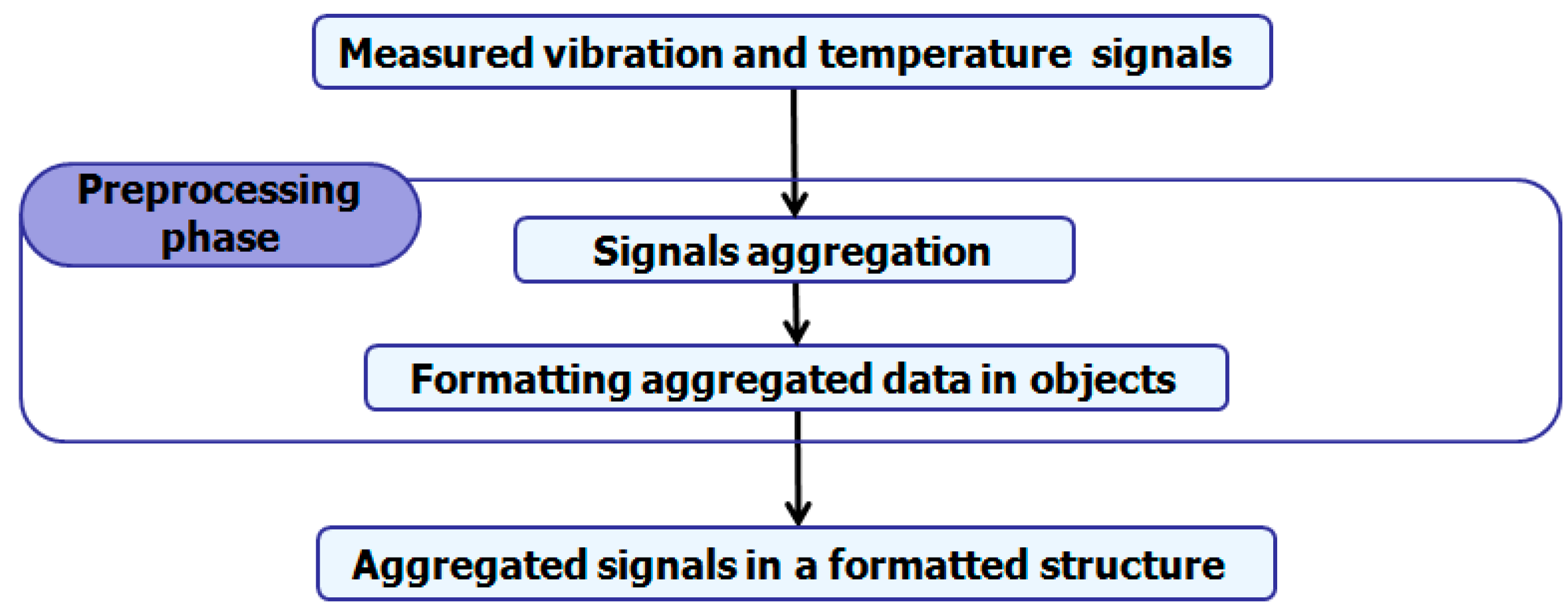
28]. These solutions unfortunately increased the computation cost. Therefore, in this paper, we propose a two-step pre-processing phase which is computationally cost-effective by reducing the problem complexity, which can be summarized as follows (
Figure 2):
This step consists of eliminating the measured signals noise, thus reducing the problem complexity. Firstly, the vibration and temperature signals are aggregated over a time interval then represented by a unique data computed by one of the aggregation functions: mean, variance, or standard deviation, selected as a parameter in the aggregation procedure. The main constraint is the time interval definition that should be at the same time small enough to avoid losing data knowledge and long enough to ensure algorithm complexity optimization and noise overcoming. If the algorithm complexity is C(n), where n is the measured signals number, the complexity then becomes C(m) after aggregation, where m= n/k and k is the measured signals number in a time interval. The time interval is selected according to the measured signals data structure.
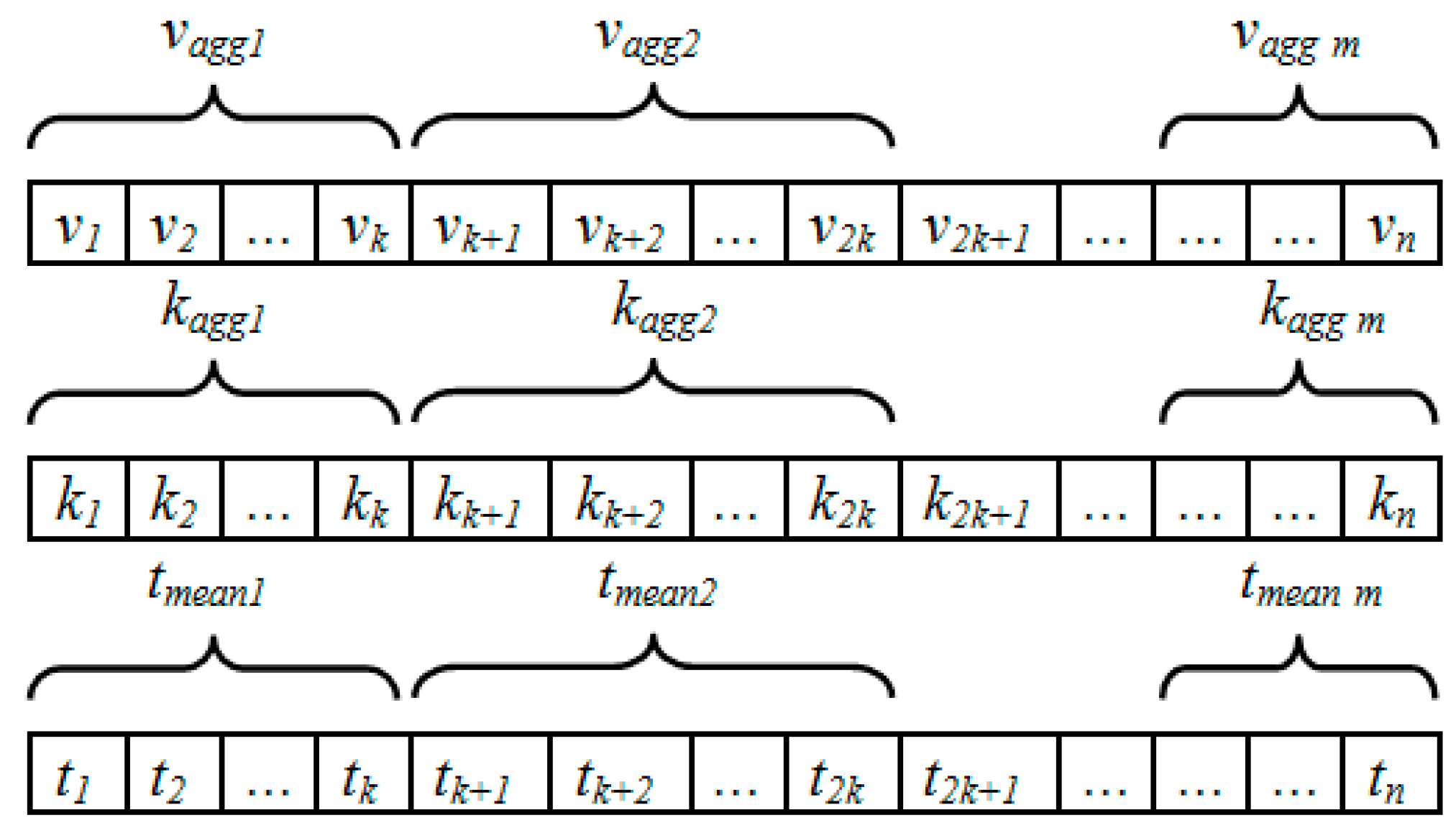
Given
V = (
v1,
v2, …,
vi, …,
vn) the measured vibration signals,
K = (
k1,
k2, …,
ki, …,
kn) the measured temperature signals, and
T = (
t1,
t2, …,
ti, …,
tn) the time vector, where
ti is the sampling time of
vi and
ki.
Figure 3 represents the signals aggregation process, where according to the selected aggregation function,
vaggi and
kaggi are, respectively, the aggregated vibration and temperature signals and
tmeani represents the average time value of the time interval
i.
This second step seeks to prepare the aggregated data in a formatted structure that can be used in the diagnosis phase. In this step, a data structure containing formatted objects O = (o1,o2, …, oi, …, om) is created, where each object oi(vaggi,kaggi,tmeani) contains the aggregated vibration and temperature signals vaggi and kaggi and the average time value tmeani.
The resulting data structure O can be represented in a three-dimensional space where each object oi contains three axis coordinates (vibration, temperature and time), which can be directly used in the diagnosis phase.
3.2. Diagnosis Phase
In this phase, we design first a VNS [
28] metaheuristic, which consists on measured vibration and temperature signals clustering for bearing failures diagnosis. Nonetheless, VNS, as a trajectory method, is still prone to premature convergence traps due to its limited exploration ability caused generally by the initial solution. Thus, it is hybridized with a CMO metaheuristic [
27], where VNS is used in a pipeline mode after CMO which generates the initial solution to balance between diversification (global exploration) and intensification (local exploitation), during the evolutionary process.
VNS has shown the potential to exploit promising regions in the search space with higher quality solutions [
32,
33,
34,
35,
36,
37,
38,
39,
40,
41]. The basic idea of VNS consists of systematically changing the neighborhood structures, thus enabling it to avoid trapping in local optima. It starts with an initial solution and then refines it through three main phases so-called neighborhood change, local search, and shaking until a stopping criterion is met [
32]. VNS is used to solve different combinatorial optimization problems such flowshop scheduling problem [
33] where the initial solution is constructed by a GA; in the vehicle routing problem [
34], the nearest neighborhood heuristic proposed in [
35] is applied to construct an initial solution; the workforce scheduling and routing problem [
36]; the course timetabling problem [
37] using a constructive heuristic to define the initial solution; the edge-ratio network clustering [
38] with a hierarchical divisive algorithm to construct the initial solution; the redundancy allocation problems [
39]; the cyclic bandwidth sum minimization problem [
40] and the labeling graph problems [
41] with a random initial solution.
To the best of our knowledge, VNS has not been applied alone nor hybridized with other methods for the bearing failures detection and diagnosis problem. This encouraged us to design a VNS to tackle this problem in induction machines by using the unsupervised classification of measured vibrations and temperature signals in classes.
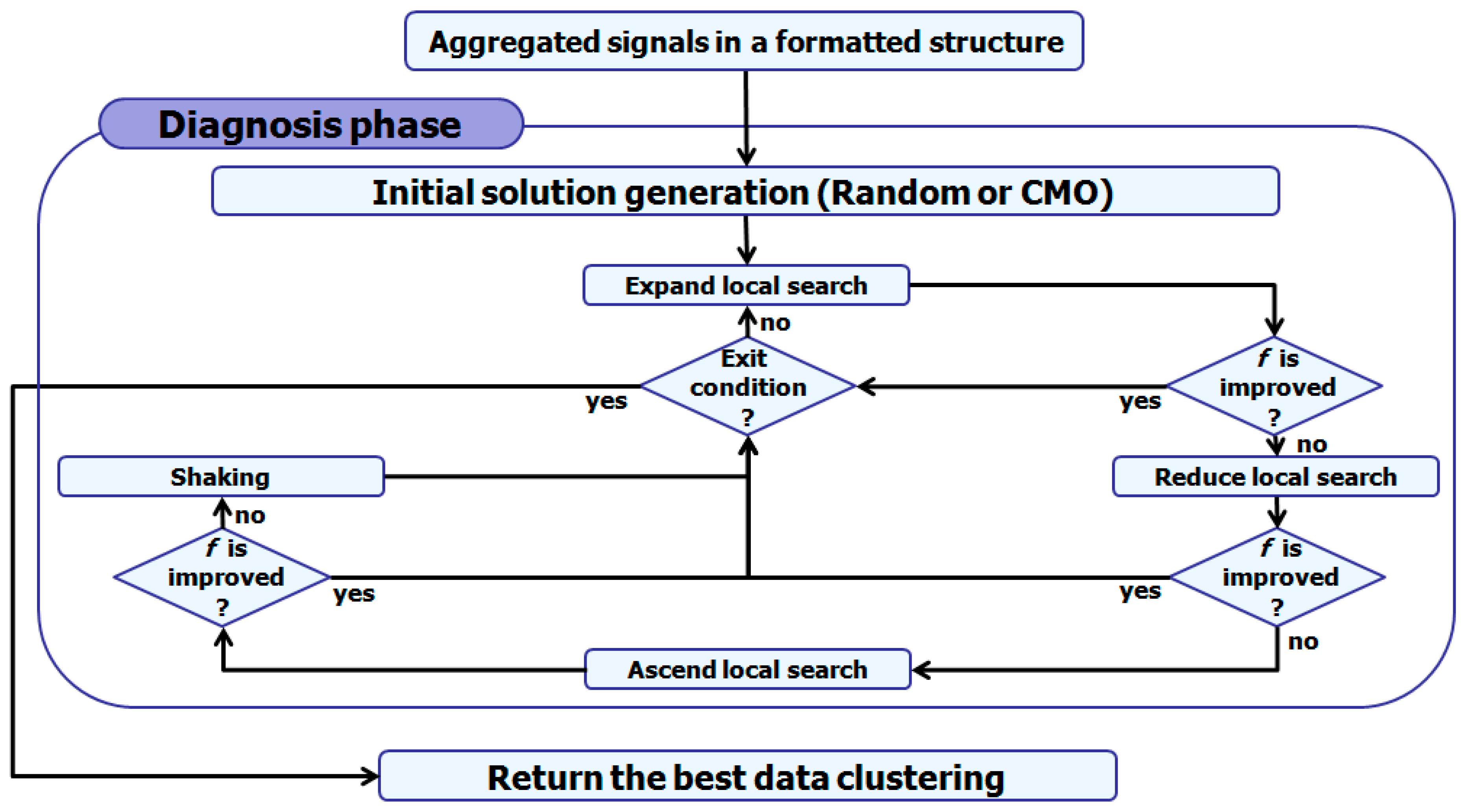
Algorithm 1 outlines the proposed VNS method [
28]. It follows a simple strategy for neighborhood change, which is performed deterministically. The search algorithm moves from one neighborhood to another when there is no possible improvement of the processed solution in the current neighborhood. After each improvement, the search process returns to the first neighborhood.
Figure 4 illustrates the diagnosis phase workflow:
In the following subsections, we give the specifications of the proposed VNS. First, the solution representation and the objective function, then the initial solution generation methods, neighborhood structures, local search procedures, and the shaking technique are discussed.
|
Algorithm 1. VNS Main Algorithm
|
| Input InputDataset, Exit_conditions |
| Begin |
| E = Pre-processing (InputDataset) |
| X0 = Generate_Initial_Solution(E) |
| Xbest = X0 |
| Xcurrent = X0 |
| i = 0 |
| Repeat |
| k = 1 |
| Stagnation = True |
| Xprev = Xcurrent |
| While k ≤ 3 Do// Neighborhood Search |
| Switch (k) |
| Case 1: Xcurrent = Expand_Local_Search (Xprev) |
| Case 2: Xcurrent = Reduce_Local_Search (Xprev) |
| Case 3: Xcurrent = Ascend_Local_Search (Xprev) |
| End Switch |
| Iff(Xcurrent)>f(Xprev) |
| Then k=1 |
| Stagnation = False |
| Else k = k + 1 |
| End If |
| End While |
| If(Stagnation) |
| ThenXcurrent = Shake (Xprev) // Shaking |
| i=i+1 |
| Elsei = 0 |
| End If |
| Iff(Xcurrent) > f(Xbest) Then Xbest = Xcurrent |
| UntilExit_conditions |
| Return Xbest |
| End. |
3.2.1. Solution Representation and Objective Function
To effectively solve the problem, it is important to select a proper solution representation. A candidate solution X (x1,x2, …, xi, …, xn) where n represents the class number, is a list of one-dimension array of objects, each array xi(xi1,xi2, …, xik), where k represents the class cardinal, represents one class containing all included data xij(vij,kij,tij), where each piece of data is an object containing the aggregated vibration and temperature signals vij and kij and the average time value tij.
In general, the objective function is defined by calculating inter-data distance in a same class in order to minimize the global intra-class distances. However, the purpose of clustering is to minimize the intra-class distances while maximizing the inter-class ones. It is therefore necessary to define a more consistent objective function to ensure the inter-class distance maximization, thus obtaining well-separated classes.
Given
ci the centroid of the class
xi in the solution
X. The objective function is computed as follows [
28]:
Calculate the inter-class distance
DInterClass:
Calculate intra-class distance
DIntraClass:
Class
xi average distance containing
k objects is:
For each class, the aim is to maximize the inter-class distance compared to the average one. Partial objective function for the class
xi is therefore given by:
The global objective function is given by:
The aim is to maximize the proposed objective function f(X), defined by dividing the inter-class distance by the sum of the intra-class distances. In a clustering configuration X, the inter-class distance represents the sum of distances between all the class centers (c1,c2, …, cn), while the intra-class distance for the class xi represents the sum of distances between all of its data(xi1,xi2, …, xik). By dividing the inter-class distance by the sum of all the intra-class distances, f(X) becomes directly proportional to the first and inversely proportional to the latter. Seeking to maximize f(X), means moving towards a clustering configuration where the inter-class distance is being maximized, meaning that the resulting classes are becoming distantly separated, while the intra-class distances are being minimized, meaning a strong data similarity inside each class.
3.2.2. Initialization Procedure
The dependency of VNS performance, as a trajectory method, on the initial solution as it is sequentially improved makes it important to focus on the initial solution generation strategy. In this paper, we propose two strategies to generate the initial solution: random generation or using the clustering oriented CMO metaheuristic. Consequently, two versions of VNS are designed: (1) RAN_VNS in case the initial solution is generated randomly, and (2) CMO_VNS in case the initial solution is generated using CMO.
This process consists of assigning objects to classes. The number of classes is increased in each iteration and varies in an interval from two to the predefined maximum number that defines the exit condition. In each iteration, classes centers are randomly selected according to the current classes number, then each data is assigned to its nearest class center. If the current iteration solution has the best objective function value, it becomes the best solution. The output is the data configuration that has the best objective function (Algorithm 2) [
28]. This procedure allows defining a dynamic number of classes because the number of resulting classes varies according to the best-found solution.
|
Algorithm 2. Random initial solution generation.
|
| Input Dataset B // measurement data |
| Begin |
| Initialize Max_Classes_Number |
| Repeat |
| k = 2 // Initialize k the classes number |
| While k ≤ Max_Classes_Number Do |
| Classes_center = Select_Class_Center(B,k) |
| Xk =Affect_Data(B,Classes_center) |
| Calculate f(Xk) |
| Iff(Xk) > f(Xbest) |
| ThenXbes t= Xk |
| End If |
| k = k + 1 |
| End While |
| UntilExit_conditions |
| ReturnXbest |
| End |
The main problem of the random generation is to define the classes number because it is a random technique for choosing the classes number and also for choosing the class centers.
CMO is a metaheuristic inspired by the natural phenomenon of a body’s movement in space [
42] proposed initially for image segmentation problem using pixels clustering to extract objects from a given image. CMO [
27] starts by transforming the preprocessed measured signals into a space body system. Then, its algorithm is executed in two successive steps:
- (1)
Find equilibrium of rotating satellites around planets by applying Earth–Moon system then group each planet with its satellites as one body after stabilization;
- (2)
Group formed bodies by applying Earth–Apple (system merging bodies according to the gravitational attraction force).
For the sake of concise presentation, CMO is briefly presented in
Section 3.3.
3.2.3. Neighborhood Structures
Since neighborhood structures play a key role in VNS, it should be rigorously chosen for efficiency purposes. Neighborhood structures are based on class solidity notion, which represents data dispersion degree. The class with the smallest data dispersion will represent the strongest class and the one with largest data dispersion will be considered the weakest class. The optimized data dispersion function for class
i is defined as follows:
where
ci represents class
i center and (
xi1,
xi2, …,
xik) represent the class data where the cardinal is
k.
The proposed neighborhood structures are [
28]:
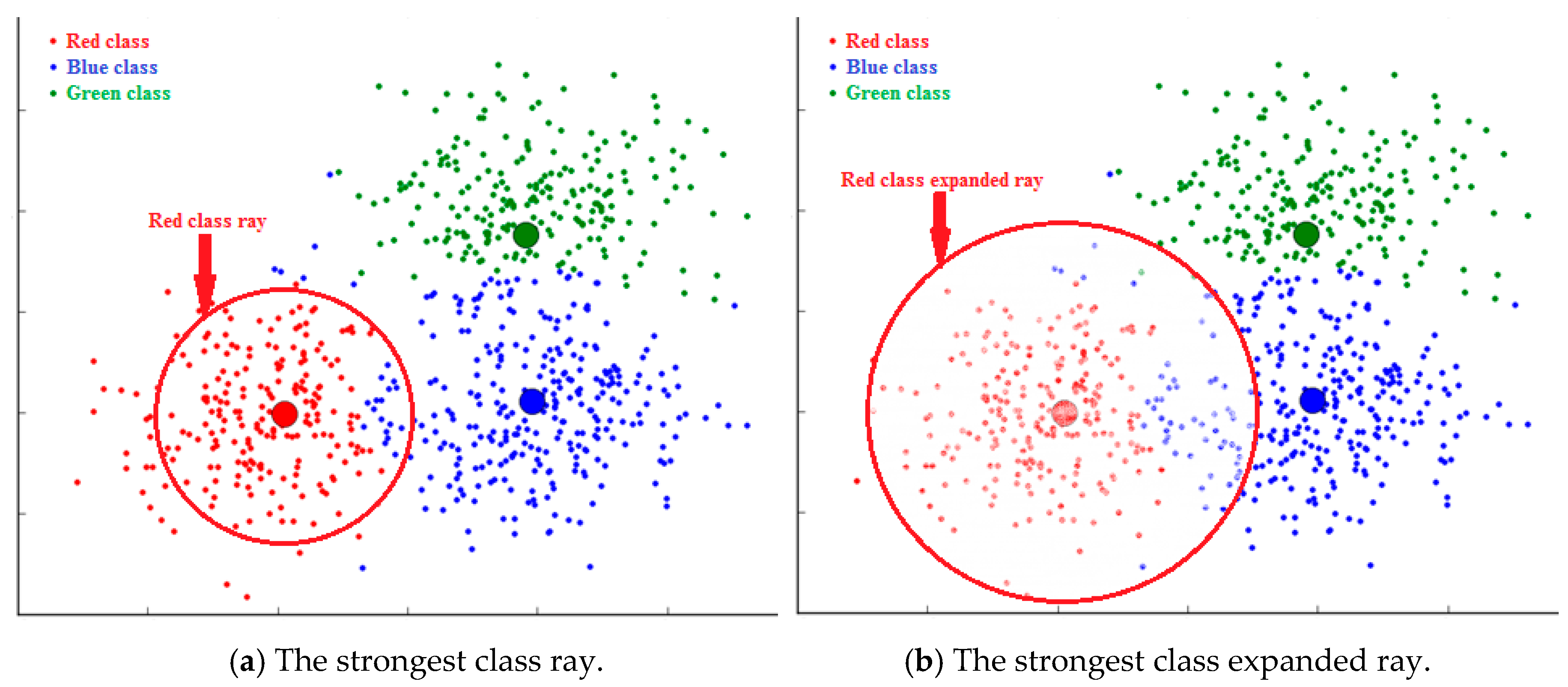
Expand. It consists of increasing the strongest class radius and then including all data located inside.
Figure 5 is an illustrative example where the red class is the strongest one. It will be expanded such that all data located inside the expanded ray will be assigned to it.
Reduce. It consists of decreasing the weakest class radius and then releasing the data located outside the new radius and assigning them to the nearest class. Let’s take the same example introduced in
Figure 5 where the blue class is the weakest one. The blue class will be reduced such that all blue data located outside the reduced ray will be assigned to the nearest class, as shown in
Figure 6.
3.2.4. Local Search Procedures
Each VNS method embeds three local search (LS) procedures: (1) Expand_Local_Search, (2) Reduce_Local_Search, and (3) Ascend_Local_Search described in what follows:
In this case, the algorithm receives the current solution as input and extracts the strongest class. Its radius will be increased according to the expand coefficient parameter. This class will afterward include all data located inside the new radius (Algorithm 3).
|
Algorithm 3. Expand_Local_Search(X)
|
| Begin |
| k = Get_Strongest_Class_Index(X) |
| Radius =Get_ Radius(Class(k)) |
| New_ Radius = Radius*Expand_Coef |
| n = Get_Clases_Number |
| Fori = 1 To n |
| m = Get_Objects_Number(class(i)) |
| For j = 1 To m |
| If Distance(X(i,j),Class_Center(k)) < New_Radius |
| Then Affect(X(i,j),Class(k)) |
| End If |
| Next j |
| Next i |
| Return X |
| End. |
In this case, the algorithm receives the current solution as input and extracts the weakest class. Its radius will be decreased according to the reduce coefficient parameter. This class will afterwards release all the data located outside the new radius. All released data will be assigned to the class with the nearest class center (Algorithm 4).
|
Algorithm 4.
Reduce_Local_Search (X)
|
| Begin |
| k = Get_Weakest_Class_Index(X) |
| Radius = Get_ Radius(Class(k)) |
| New_ Radius = Radius/Reduce_Coef |
| m = Get_Objects_Number(class(k)) |
| Fori = 1 To m |
| If Distance(X(k,i),Class_Center(k)) > New_ Radius |
| Then Affect(X(k,i),Nearest_Class) |
| End If |
| Next i |
| Return X |
| End. |
In this case, the algorithm receives the previous solution as input and then inverts the used LS procedure. For example, if the used LS in the previous iteration is Expand_Local_Search then it uses Reduce_Local_Search. Of course, this procedure cannot be applied in the first iteration (Algorithm 5).
|
Algorithm 5.
Ascend_Local_Search (X).
|
| Begin |
| NewX = Get_Previous_Solution(X) |
| Previous_Structure = Get_Previous_Structure(X) |
| IfPrevious_Structure = "Expand" |
| ThenReduce(NewX); |
| Return NewX |
| Else IfPrevious_Structure="Reduce" |
| Then Expand(NewX); |
| Return NewX |
| Else If Previous_Structure = "Ascend" |
| Then Shake(X); |
| Return X |
| End If |
| End If |
| End If |
| End. |
3.2.5. Shaking Procedure
The shaking procedure objective is to disrupt the current solution by switching to another local neighborhood (diversification) when all visited did not improve the current solution. This procedure aims to provide a wide exploration of the search space in order to avoid local optima. The proposed shaking procedure consists of swapping the most distant object from the class center to the closest class one. This perturbation is applied if the previously used structure is the third one (Ascend) to avoid looping (Algorithm 6) [
28].
|
Algorithm 6.
Shake(X).
|
| Begin |
| n = Get_Class_Number |
| Fori = 1 To n |
| k = Get_Furthest_Index_Object(X(i)) |
| Affect(X(i,k),Nearest_Class) |
| Nexti |
| ReturnX |
| End. |
3.3. Detection Phase
To ensure failure detection, VNS-clustering graphical representation is used to extract features and build a knowledge base in the learning step, which will then be used to calculate failure type probabilities in the decision step. At the end of both steps, a dynamic knowledge update is performed to ensure continuous learning and enhance the algorithm decision making. To perform this, learning and decision algorithms based on CMO metaheuristic are proposed.
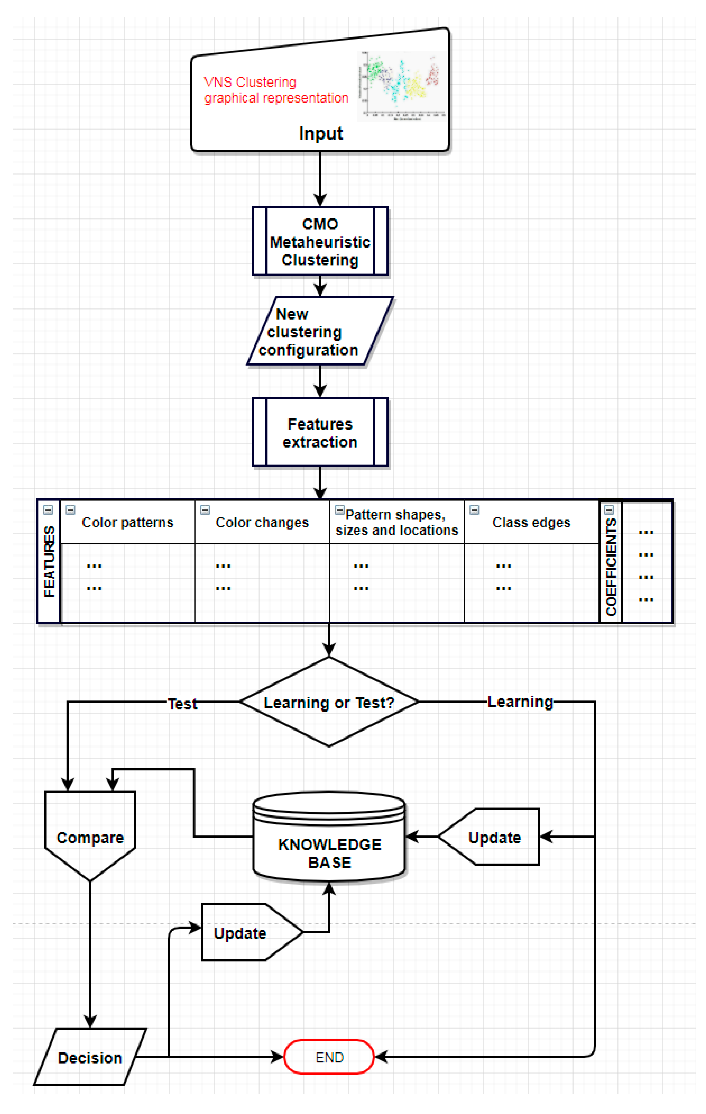
The general block diagram of the detection phase is illustrated by
Figure 7. In what follows, we first present an example to illustrate our detection approach. Further, we present briefly the CMO metaheuristic. For a more detailed description of CMO, we refer the interested reader to the seminal papers in [
27,
42]. Then, we will proceed to detailing the learning step and the detection step.
Figure 8 introduces an illustrative example for the detection phase, where learning datasets are processed during the learning step to provide patterns for different bearings failure types. These patterns are defined by their distinctive features which are inserted in the knowledge base. During the test step, test datasets are processed, and their features are extracted and matched with the knowledge base to make failure type decision.
In this example, CMO metaheuristic is applied in both learning and test steps on the input VNS-clustering graphical representation image (
Figure 9) to make clustering containing new bearings health state configuration (
Figure 10).
Each class representing a health state is processed at pixel level to extract its defining features for a given failure type: color patterns which represent a dominant health states model, color changes which represent a bearing transition model from an operating mode to another, the class edges which represent the classes shape model, as well as pattern shapes, sizes, and locations, which represent a classes shape model.
3.3.1. CMO Metaheuristic
The CMO metaheuristic is based on the classical mechanics laws to simulate the natural phenomenon of bodies movement in space [
27,
42]. The proposed CMO uses the VNS-clustering graphical representation as 2-dimensional image input (
Figure 9) which represents the degradation evolution over time according to the measured vibration signals. Each class represents a system health state that contains a set of measured vibration signals during a given health state and is represented in a distinctive random color. In each input image, different system health states are gathered into separated classes using CMO metaheuristic (
Figure 10). The main purpose is to define a representative model for each failure type by browsing each resulting cluster at pixel level to extract its defining features and converting them into stored data in the knowledge base.
CMO starts by transforming the preprocessed measured signals into a space body system. Then, its algorithm is executed in two successive steps (Algorithm 7): applying Earth–Moon system equilibrium then grouping formed bodies and applying Earth–Apple system equilibrium.
|
Algorithm 7.
Classical Mechanics-based Optimization (CMO).
|
| Input B // Diagnosis phase: B represents preprocessed measured signals |
| //Detection phase: B represents the VNS clustering graphical representation image |
| Begin |
| Calculate (m) // calculate the planet number according the formatted objects number |
| Calculate (n) // calculate the satellite number |
| Calculate (DistanceRatio) |
| Find the Earth-Moon system equilibrium (B) |
| Find the Earth-Apple system equilibrium (B) |
| End. |
To create planets and satellites, we regularly select m objects P = (p1,p2, …, pm) as planets from the input set of objects O = (o1,o2, …, ok), where k represents the objects number. In the diagnosis phase, each object oi(vi,ki,ti) contains the aggregated vibration and temperature signals vi and ki and the average time value ti. In the detection phase, each object oi(xi,yi,ci) contains a pixel in the input image where xi and yi represent its coordinates and ci represents its color. The remaining n objects (n = k - m) will be considered as the satellite set S = (s1,s2, …, sm).
After transforming the input data into a space body system, each body represents one class, which contains its included satellites. Each class center is its corresponding planet. Each class has two gravitation fields calculated according to its mass, which correspond to an attraction force applied. The first field is applied on the Earth–Moon system to keep the satellites in rotation around planets using the input data; the second one is applied on the Earth–Apple system, causing some bodies to fall on others applying the greatest attraction force.
In the earth–moon system equilibrium step, each class c1 exerts an attraction force Fc1s on a satellite, which is rotating around another planet p2 with an applied force Fc2s. If Fc1s > Fc2s, then the satellites leave its path around p2 and follows a new path around p1. This step is repeated until an Earth-Moon system equilibrium is reached, resulting in no more possible object displacements between classes.
In the earth-apple system equilibrium step, all the bodies in each planet-moon class are fused together as one body after the earth-moon system stabilization. Each class situated in the gravitational field of another one falls on it (classes fusion). After each fusion, classes gravitational fields (Earth–Apple system) are calculated. The two previous steps are repeated until the overall system is stable and no more class fusion is possible.
3.3.2. Learning Step
The learning algorithm (Algorithm 8) uses the VNS-clustering graphical representation as two-dimensional image input. It processes different classes features from the image input to build a knowledge base containing the learning data for each failure type. The used features are:
Color patterns: This feature is represented by data that describes the different main colors in a class, their appearance patterns and sequences, the way they are distributed as well as the condensation of each one compared to the dominant color which represents the most appearing color in the class, which represents each class dominant operating mode model for a given failure type.
Color changes: Defines the transition model of color changes inside the class, indicating the way the color transition is made in different parts of the class, which represents a bearing transition model from an operating mode to another for a given failure type.
Pattern shapes, sizes, and locations: A model that defines how a class is constructed from different parts, each one having a shape and size and is located in a specific zone inside the class, which represents each class structure model for a given failure type.
The class edges: A rather more general model that describes the overall shape of the class by extracting its edges and normalizing them to a predefined size to be able to cross check them with any other shape even when one or both of the compared shapes is irregular, which represents the classes shape model for a given failure type.
Inside each class image, the algorithm searches for the particular occurrences of the said features and the way they appear in a class define how it is constructed. Every health state in the knowledge base has its own feature coefficients configuration that the algorithm updates after every iteration to keep track of the importance of each feature to differentiate a given class.
For each class, the algorithm passes by three major steps:
CMO metaheuristic data clustering: to define a new clustering configuration of the input image. Each resulting new class can contain multiple colored parts from the original classes in the input image as part of its defining features.
Extraction of each new class features that are processed and transformed to numeric data ready to be stocked in the knowledge base.
Inserting the new data in the knowledge base and updating the coefficients according to the importance of each feature in defining the class, based on the matching between the decision extracted feature and the one already existing in the knowledge base. During the first learning session, the algorithm analyses the resulting information and assigns a default coefficient to each feature based on their degree of variation, thus the more regular a feature is, the bigger the coefficient it receives.
|
Algorithm 8.
Learning
|
| Input LearningSet |
| Begin |
| E0 = VNS(LearningSet) //E0 represents the VNS clustering graphical representation pixel matrix |
| of the LearningSet |
| E = CMO(E0) // E represents the new data configuration with CMO |
| FC = ProcessCFeatures(E) //FC represents the matrix containing the color features of each class |
| FCC = ProcessCCFeatures(E) //FCC represents the matrix containing the color changes features of each class |
| FSSL = ProcessSSLFeatures(E) //FSSL represents the matrix containing the size, shape and location features |
| of each class |
| FE = ProcessEFeatures(E) //FE represents the matrix containing the edge features of each class |
| Coeff = CalculateFeatureCoefficients //Coeff represents the array containing the updated feature coefficients |
| LearningStructure = Assemble(FC, FCC, FSSL, FE, Coeff) //Create a new structure containing |
| all the features matrix |
| ReturnLearningStructure |
| End. |
3.3.3. Decision Step
The decision algorithm (Algorithm 9) is used to detect the failure type from an input image of a given test dataset VNS-clustering graphical representation, it also shares the same first two data processing steps with the learning algorithm: the CMO metaheuristic data clustering step and the extraction step of the color patterns, color changes, the class edges and pattern shapes, sizes, and locations features. After the features are extracted, the algorithm uses them to calculate matching probabilities with the knowledge base, where during each matching the test image colors are normalized according to a learning images colors degradation over time, a failure type decision is then taken according to the highest probability. Finally, the algorithm performs cognitive feedback by comparing the detected failure type original features and coefficients in the knowledge base with the ones extracted from the input image to enhance the knowledge data and optimize the coefficients. The steps taken by the decision algorithm are:
CMO metaheuristic data clustering results in a new clustering configuration.
Extraction of each new class features.
Computing the feature matching probabilities with every failure type in the knowledge base. In this step, the probability is decreased by the differences between the extracted features and a given knowledge failure type, taking into consideration the importance coefficient of each feature. The failure type detection decision is then taken according to the highest matching probability.
Updating the knowledge base by comparing the extracted features with the detected failure type features stored in the knowledge base. In this step, the algorithm also optimizes the feature coefficients taking in consideration the contribution of each feature in pointing the resulting probability towards a correct decision.
|
Algorithm 9.
Decision
|
| Input TestSet, KnowledgeBase |
| Begin |
| E0 = VNS(TestSet) //E0 represents represents the VNS clustering graphical representation pixel matrix of the |
| TestSet |
| E = CMO(E0) // E represents the new data configuration with CMO |
| FC = ProcessCFeatures(E) //FC represents the matrix containing the color features of each class |
| FCC = ProcessCCFeatures(E) //FCC represents the matrix containing the color changes features of each class |
| FSSL = ProcessSSLFeatures(E) //FSSL represents the matrix containing the size, shape and location features |
| of each class |
| TestStructure = Assemble(FC, FCC, FSSL, FE, Coeff) //Create a new structure containing all the features |
| matrix |
| Probabilities = CalculateProbabilities(TestStructure, KnowledgeBase) //Matching according to the knowledge |
| base |
| UpdateKnowledge(Probabilities) //Cognitive feedback to update the knowledge base |
| ReturnProbabilities |
| End. |
4. Validation on Experimental Data
The aim of this section is testing how effective is the proposed three-phase approach for solving induction machines bearing failures detection and diagnosis problem. The algorithms have been implemented on MATLAB 2015 and C# .NET 2015 and run experiments on 64 bits operating system PC with 8 Gb of installed memory and i7 processor @ 2.00GHz. To ensure results, stability algorithms have been independently run 10 times on each dataset. The experiments are classified into two sets of tests of which each is dedicated to each phase of the proposed approach.
In what follows, we will first describe the used datasets and data pre-processing. Then, we evaluate the different features of our newly proposed VNS algorithm. Finally, experimental results are analyzed and discussed.
4.1. Datasets
PRONOSTIA experimental platform vibration and temperature data have been used for validation of the proposed failures diagnosis approach [
43,
44] (
Figure 11). PRONOSTIA is an experimentation platform devoted to test and validate bearings failure diagnosis and prognosis approaches [
10,
17,
26]. It provides datasets obtained by run-to-failure experiments that stop at total bearing failure, resulting in measuring a vibration maximum value (20 g). In this platform, two accelerometers measure the bearing horizontal and vertical vibrations and a thermocouple measures its temperature. The vibration and temperature signals were sampled at 25.6 and 10Hz, respectively. Files containing the signals measured during 10 min intervals are generated inside each experiment folder.
In terms of data management, they have been stored in a database using an MS-SQL-Server system where pre-processing and data storage are developed with VB.Net 2015. Details on data management and used sets for training and testing can be found in [
43,
44]. PRONOSTIA data sets are summarized in
Table 1.
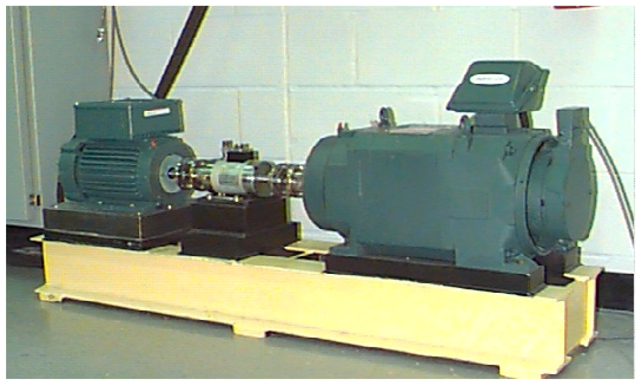
CWR vibration data were provided by the Case Western Reserve University Bearing Data Center [
45]. It is an experimentation platform devoted to test and validate bearings failure detection approaches (
Figure 12). Practical details on the experimental platform and bearing specific failure data can be found in [
45,
46]. For the evaluation of the failure detection performances, the CWR measured vibration signals are used. Two different sets of experimentations were performed on all failure types. The first set collected all the failure types data at a sampling time of 12,000 samples/second and the second one at 48,000 samples/second. In this work, all the dataset collected at 12,000 samples/second are used as learning datasets and the ones collected at 48,000 samples/second are used as test datasets. CWR learning and test datasets are summarized in
Table 2 and
Table 3, respectively.
The measured experimental vibrations and temperature signals first go through the preprocessing phase. In the resulting data objects, the temperature signals have very large values compared to the vibration ones. Consequently, temperature can have a larger influence on the clustering. This is true for time data, which has very large values with respect to vibrations and temperatures. This is why data normalization is a mandatory step that aims to put the different data on the same range to be able later correctly giving a relative impact to a given vector by using corresponding coefficients. This is important to ensure that all handled data have the same influence on clustering.
In the aggregated data structure O = (o1,o2, …, oi, …, om), given V = (v1,v2, …, vi, …, vm) the aggregated vibration vector, K = (k1,k2, …, ki, …, km) the aggregated temperature vector and T = (t1,t2, …, ti, …, tm) the average time vector of the interval values. Vaverage, Kaverage, and Taverage represent the averages of V, K, and T, respectively. The new normalized vectors become:
Vnormalized = V.Taverage.Kaverage.Coeffvibration
Knormalized = K.Vaverage.Taverage.Coefftemperature
Tnormalized = T.Vaverage.Kaverage.Coefftime
where Coeffvibration, Coefftemperature, and Coefftime represent the relative impact coefficients.
Example: giving two vectors x={0,2,4} and y={100,200,300}, the normalization here gives x’= {0,400,800} and y’={200,400,600}, i.e., multiply the vector x by the average value 2 of the vector y and multiply the vector y by the average value 200 of the vector x.
4.2. Pre-Processing
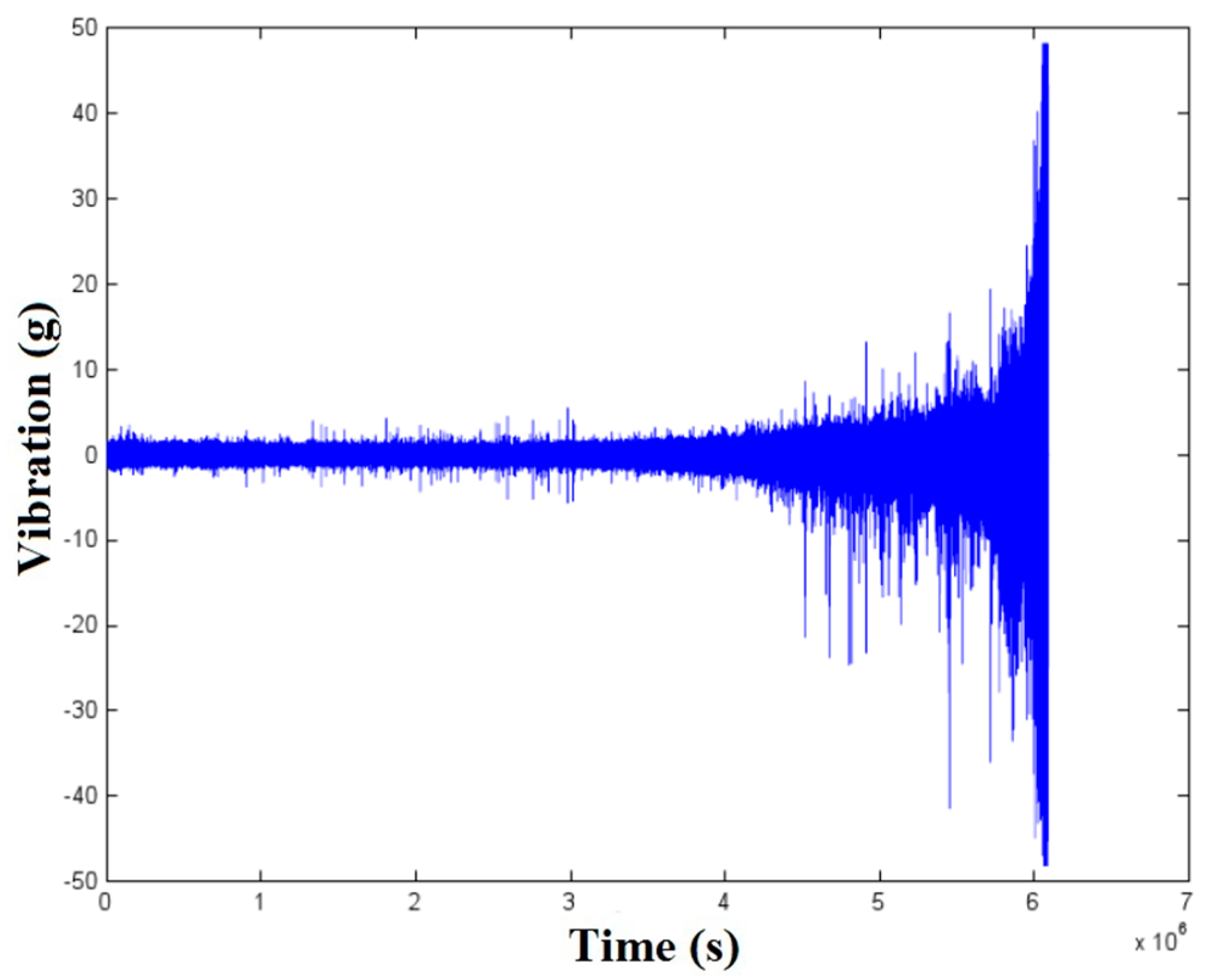
In PRONOSTIA platform, each data file contains the measured signals for 10 min with a sampling frequency of 25.6Hz for temperature signals and 10Hz for vibration signals. To optimize the algorithm progressing time, measurements have been aggregated per file considering the aggregated file as a single signal measurement using a standard deviation function. In this context, each signal measurement file becomes a single datum. After the data aggregation step, fair data normalization is applied to vibration, temperature signals, and time.
An example of a vibration raw signal from a PRONOSTIA platform experiment is shown in
Figure 13.
4.3. Diagnosis Phase Using VNS Clustering
The two proposed VNS versions (RAN_VNS and CMO_VNS) are applied and tested with each neighborhood structure Expand and Reduce separately before combining them, to evaluate the performance of the proposed approaches.
After the pre-processing phase, newly aggregated and normalized data is obtained. The first way to define an initial solution is a random generation where the selected solution has the best objective function and the class number is auto-selected according to the best solution. The obtained random initial solution for the learning set B1_1,using the variance aggregation function and by applying fair relative impact coefficients for normalization, is shown in
Figure 14. The obtained number of random generation classes is big, and the classes are not well-separated which will influence VNS convergence.
The second way to define an initial solution is by using CMO metaheuristic. The obtained result for the learning set B1_1 is shown in
Figure 15. The classes number of the obtained CMO results is not big and the classes are well-separated. This will be helpful to the VNS convergence.
Using CMO initial solution generation, we will first separately test the performance of each neighborhood structure expand and reduce before combining them. The third local search consists of inverting the last used structure between the first neighborhood structure and the second one, so it is not possible to test it separately.
At each iteration in the expand neighborhood, the strongest class radius is expanded. However, it will not lead to the single class configuration that contains all data, because the assigned data make the strongest class weaker when running the next iterations. The obtained results are shown in
Figure 16. The obtained result for learning set B1_1 using only the Expand neighborhood shows only two classes, the healthy mode and the faulty one.
At each iteration in the reduce neighborhood, the weakest class radius is reduced. However, it will not lead to a configuration when each class contains only one data, because the loosed distant data make the weakest class stronger when running the next iterations. The obtained results are shown in
Figure 17. The obtained result for learning set B1_1 by using only the reduce neighborhood shows three classes, two classes for the healthy mode and one for the faulty one.
The results obtained by separately applying Expand and Reduce neighborhood structures show a data clustering with separated classes. We can now use them as different local search procedures for the proposed VNS.
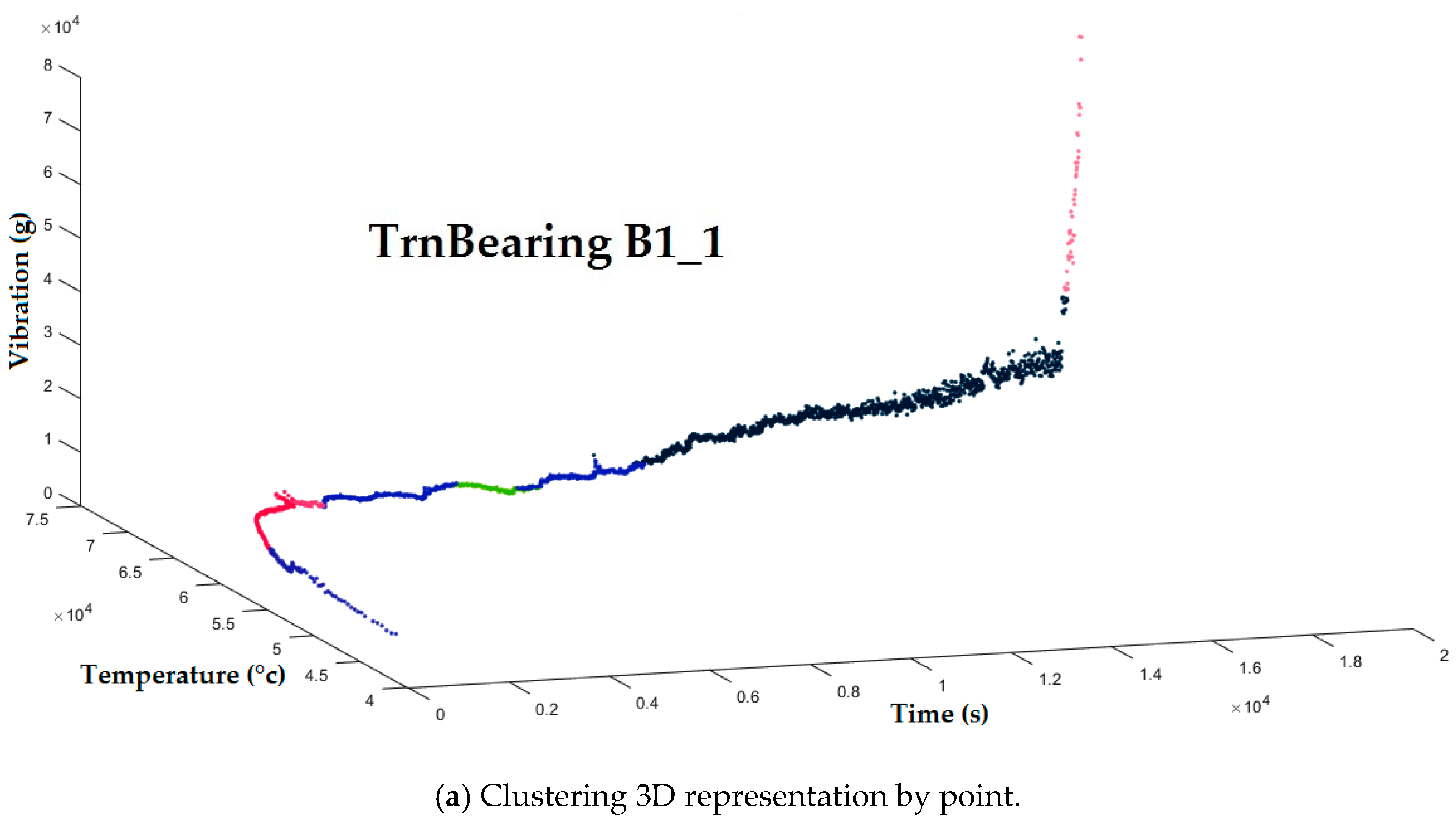
In the following, we will present tests of VNS-clustering application on PRONOSTIA datasets where CMO is used to generate the initial solution with the three proposed local search procedures Expand_Local_Search, Reduce_Local_Search, and Ascend_Local_Search for the solution space exploitation, and the shaking procedure for the solution space exploration. The results are shown in
Figure 18.
Each class in the resulting clustering represents an induction machine (bearing) operating state. The achieved results clearly show the proposed VNS-clustering high performance, where bearing degradation is highlighted over time. Indeed, for each experiment, several classes are obtained. It should then be concluded that the proposed metaheuristic-based approach is an effective tool to monitor the induction machine bearings health state until failure.
4.4. Detection Phase Performance Analysis on CWR Bearing Data Center
Since PRONOSTIA platform does not provide detection datasets, to assess the performance of the failures detection phase we used CWR Bearing Data Center datasets for all bearing failure types [
45], as detailed in (
Table 2 and
Table 3), fifteen datasets are used for the learning step and thirteen are used for the testing step. After the pre-processing phase, VNS-clustering is applied to CWR datasets. The resulting clustering contains different classes representing the system health state as shown in
Figure 19, using the variance aggregation function and by applying fair relative impact coefficients for normalization. The proposed learning algorithm processes these classes to extract the learning dataset features and insert them in the knowledge base (
Table 4). During the decision step, the VNS algorithm processes the test sets to construct data clustering and then the decision algorithm ensures failure detection by processing the resulting clustering to extract features and matching them with the knowledge base. The obtained results for bearing failure detection using the learning algorithm are summarized in
Table 5.
Prob_1, Prob_2, and Prob_3 represent failure type probabilities, the results show the three probable failures in descending order for each test set detection result where the final decision taken by the algorithm is the most probable failure detection and having a probability ofProb_1. Only one learning session was performed for every failure type, according to the platform provided learning datasets. Among 13 tests, the failure detection decision probability Prob_1 for 10 tests exceeded 50%, and despite the fact that the decision probabilities of the remaining three tests were below 50%, they were correct and had a decision probability that is way higher than the next two probable failure types Prob_2 and Prob_3, meaning that the algorithm decisions were conclusive for all the 13 cases. The relatively low probabilities of some decisions were caused either by the algorithm performance, especially under the condition of ongoing only one learning session, or by the reliability of the VNS-clustering input images themselves. The obtained results show that the algorithm has made the right decision for all the datasets with an average probability of 58%.
4.5. Comparison Study
k-medoids [
13], FCM [
15], k-means [
16], GK [
22], GG [
23,
24], and AP [
25,
26] were used in a diagnostic approach based on vibration signals clustering where class centers represent the health indicators. The differences between them are the way in which the class centers are represented, a virtual calculated point for k-means and FCM and the well-placed point for k-medoid, GK, GG, and AP. The second difference is the methods in which distances are calculated, where FCM uses Euclidean distance, GK uses a covariance matrix, GG uses the maximum likelihood estimation, and AP is based on the confidence value concept which represents the dissimilarity between the point representing the class center compared to the new candidates points to be class center. These methods are based on the evaluating performance degradation notion by the vibration signals clustering into three classes, which represent normal, slight and severe health state and the classes centers represent the health indicators.
Xu et al. [
26] applied k-means, k-medoids, FCM, GK, GG, and AP clustering on PRONOSTIA datasets [
44] to diagnoses bearing failures. After empirical mode decomposition of signals, a singular value decomposition is applied to obtain SV1 (Singular Value 1) and SV2 (Singular Value 2), the cluster center points of the three states (normal, slight, and severe) are found according to SV1 and SV2. Xu et al. achieved results are given in
Figure 10 [
26].
Compared to the proposed VNS-clustering results (
Figure 18) on the same dataset, we observe that for k-means, k-medoids, FCM, and AP clustering results (
Figure 10) [
26] give well-separated classes, but they have almost the same results because they are based on the same initial solution and are sensitive to the latter. Moreover, the slight class center is not well centered which can give a very advanced deterioration alert, so they could not effectively track the early stages of severe class. For GK clustering (
Figure 10) [
26] the resulting slight and severe classes are in the wrong order, making the clustering inaccurate. A single class representing the severe health state resulted from the GG clustering (
Figure 10) [
26] for all the datasets, meaning that the different health states cannot be diagnosed [
26].
The advantage of the proposed VNS is the use of an objective function that simultaneously respects both parts of the clustering definition, the first part consists of minimizing the intra-class distance and the second one consists of well separating classes by maximizing the inter-class distance, using data similarity measure (distance). Using CMO, a clustering-oriented metaheuristic, to generate an initial solution helps in effectively VNS. As a consequence, the obtained classes do not only represent the induction machine healthy or faulty modes, but they represent the machine (bearings) state evolution (bearings degradation) over time.
5. Conclusions and Future Work
This paper has proposed a three-phase metaheuristic-based approach for induction machine bearing failure detection and diagnosis. The first phase ensures the complexity and noise reduction by aggregating the measured signals, as well as preparing a formatted data structure for the clustering. The second phase ensures failures diagnosis based on a variable neighborhood search metaheuristic. The initial solution was defined in two ways: random generation or a classical mechanics-inspired optimization metaheuristic. The used neighborhood structures are Expand and Reduce, which are based on the distance notion. To ensure classes clear separation, an objective function was proposed to simultaneously minimize intra-class distances and to maximize inter-class distances. The third phase ensures failure detection using the resulting VNS-clustering to extract class features and update the knowledge base.
The proposed metaheuristic-based failure detection and diagnosis approach was evaluated using PRONOSTIA and CWR Bearing Data experimental platforms vibration and temperature measurements. The achieved results clearly demonstrate the failure detection and diagnosis efficiency and effectiveness of the VNS/CMO-based metaheuristic approach. On one hand, high performance clustering is clearly highlighted, leading to increased failure diagnosis accuracy. On the other hand, the metaheuristic ability has been shown not only for bearing failure diagnosis but also for tracking its evolution over time. Despite running only one learning session, the obtained results were encouraging and can be improved by performing more learning sessions.
Further investigations will be carried out in terms of failure prognosis. The obtained VNS-clustering will be deeply analyzed for prognosis (remaining useful life estimation) based on the resulting clustering graphical representation.


 and
and 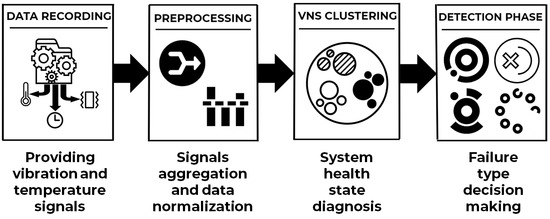


