Effect of Complex Natural Fractures on Economic Well Spacing Optimization in Shale Gas Reservoir with Gas-Water Two-Phase Flow

Abstract

At present, investigation of the effects of natural fractures on optimal well spacing of shale gas reservoirs from an economic perspective has been lacking. Traditional frameworks of fracture characterization, such as local grid refinement, make it unfeasible and inaccurate to study these effects of high-density natural fractures with complex geometries on well spacing. In this study, the non-intrusive EDFM (embedded discrete fracture model) method was presented to characterize fractures fast and accurately. The non-intrusiveness of EDFM removed the necessity of accessing the codes behind reservoir simulators, which meant it could simply create associated keywords that would correspondingly modify these fracture properties in separate files without information regarding the source codes. By implementing this powerful technology, a field-scale shale gas reservoir model was set up, including two-phase flow. The effective properties of hydraulic fractures were determined from the history matching process, and the results were entered into the well spacing optimization workflow. Different scenarios of natural fracture (NF) distributions and well spacing were designed, and the final economic analysis for each case was explored based on simulated productions. As a result, one of the findings of this study was that optimal well spacing tended to increase if more natural fractures were presented in the reservoir.

1. Introduction

Assessment for optimal well spacing is critical to efficiently develop shale gas reservoirs whose economic production has been boosted by the advanced technologies of multiple horizontal wells and multi-stage hydraulic fracturing. In that sense, the historical deployment of technology to address well spacing optimization in North America in the last decade has been significant. Moreover, the U.S. Energy Information Administration (EIA) estimated that dry shale gas production (715.8 billion cubic meters, or 25.28 trillion cubic feet) accounts for around 75% of total U.S. dry natural gas production in 2019 [1]. Likewise, according to a statistic shared by Schlumberger [2], 70% of new wells drilled in the US are infills. However, current oil and gas low-price market conditions attempt to undermine standard completions strategies and limit the industry’s capability to find techniques that make operations more rigorous and efficient in terms of profitability of the placement of new wells. The optimization of this initial stage of well spacing plays a vital role on the potential of shale gas reservoirs in order not only to prevent leaving resources undrained but also to avoid adding unnecessary costs, such as drilling infill wells in areas where gas recoveries do not exhibit significant differences when developing the field.

In these unconventional reservoirs, the economic equation also needs to take into account the impact of natural fractures and well interference through fracture communication due to the fact that space among fractured wells is getting tighter and tighter. Tighter spacing connects more preexisting fractures, which leads to the generation of complex fracture networks during the hydraulic fracturing process [3]. These “fracture hits” occurrences have been observed and predicted by many studies through wellbore image logs correlation, pressure transient analysis, pressure interference tests, and microseismic event patterns [4,5,6]. Fiallos et al. [4] exposed a field case in which these fracture hits could extend up to 1067 m (3500 ft) after a multi-well field characterization model from image logs correlations. Morales et al. [5] presented another field case, whose interwell fracture communication was clearly identified through monitoring and quantifying neighboring-wells pressure responses that overlapped the microseismic events. Similarly, Xiong et al. [6] developed a field case study, which included the frac-hit probability estimation on well spacing decisions. Furthermore, complex fracture propagation models have provided strong evidence of how complex fracture networks can be favorable to maximize shale gas production, thanks to a larger fracture surface area [6,7,8,9]. For instance, Xiong et al. [6] acknowledged that the resulted fracture network, if tight enough, could effectively drain and deplete the reservoir since the larger fracture surface area might increase the initial production rate and the ultimate recovery. Albeit there exist several recent reservoir simulation studies for well spacing optimization in shale gas reservoirs [10,11,12,13], the influence of natural fractures on well spacing decisions has been obviated. Natural fractures can significantly affect the success of hydraulic fracturing treatment. Therefore, a better understanding of the effects of natural fracture on fracture-driven interaction plays an important role in the well spacing optimization of shale gas reservoirs.

Currently, the availability of tons of information attracts to the use of data-driven approaches for reveling some uncertainties of well spacing optimization [14,15]. However, this should not be a standalone approach but rather used as a complement to advanced numerical reservoir simulation, which can accurately model the physics behind shale-gas reservoirs in order to be able to predict behavior dynamics [16]. Likewise, physics-based reservoir simulation can provide misleading results if the complexity of natural and hydraulic fracture configurations and complex two-phase flow physics are not incorporated [16,17]. In that sense, common-use reservoir fracture frameworks, such as local grid refinement (LGR) or unstructured gridding methods, might weaken the capability of modeling complex fractures explicitly [6,10,16,17,18,19]. For instance, LGR might not capture complex fracture geometries, while unstructured grids can demand too high computational resources, such as advanced parallel computing power, whose access can become a new challenge. On the other hand, the non-intrusive EDFM (embedded discrete fracture model) method provides efficient solutions to model very complex and natural fractures in terms of reliability, flexibility, and simulation run time, as exposed in different studies [20,21,22]. As a consequence, this innovative EDFM technology works in conjunction with any third-party reservoir simulator to overcome the limitations of existing methods.

In this study, economic analysis for well spacing optimization was introduced after employing the non-intrusive EDFM technology in conjunction with a third-party reservoir simulator as a solution to simulate shale gas (gas and water) production of multiple wells configurations efficiently. This research started by creating the reservoir models that would be appraised in three different well spacing scenarios (200 m, 300 m, and 400 m or 656 ft, 984 ft, and 1312 ft) and three setups of natural fracture (NF) distributions (no NF, 274 NFs, 1196 NFs). Next, one well with available field production data was subjected to AHM (automatic history matching) process [23,24,25,26] in order to match their bottomhole pressure and water flow rate record under the gas flow rate constraint, so that some representative realizations of hydraulic fracture and reservoir parameters could be achieved. Subsequently, the history-matched reservoir model with effective fracture properties was extended to include two horizontal wells with three different well spacing values of 200 m, 300 m, and 400 m (656 ft, 984 ft, and 1312 ft). In addition, the impacts of different numbers of natural fractures on multiple shale-gas wells’ performance were investigated. The effect of natural fracture density on well spacing optimization and pressure distribution was discussed. Finally, an economic evaluation was carried out by estimating the highest attainable NPV (net present value).

2. Methodology

The non-intrusive EDFM method was applied to explicitly and efficiently model complex hydraulic fractures and natural fractures, which was developed by Xu et al. [27,28], as shown in Figure 1. The non-intrusive EDFM method could be conveniently applied with the third-party reservoir simulator without modifying its source code to handle any complex fracture networks. Fractures with any shape and angles could be directly embedded into simple matrix grids without the need for local grid refinement, which increased the number of grid blocks near the fracture regions. Based on the intersections between fractures and matrix grids, the fractures were discretized in regard to each matrix grid block that was intersected by the fracture. Next, extra grid blocks called “fracture cells” were assigned for every fracture segment in the physical domain, which were described by non-neighbor connections (NNCs) in the computational domain. The flowing mechanism was connected in the physical domain between different mediums (four types described in the next sentences), but they were discontinuous in the computational domain. To solve this problem, NNC modeled fluid flow and mass transfer between fracture and matrix grid blocks based on calculations of transmissibility factors between different mediums. In particular, EDFM considered four types of connections among fractures, matrix, and well [27,28]. These connections included the NNC between matrix grid blocks and the corresponding fracture segments, NNC between fracture segments (same single fracture), NNC between intersecting fracture segments (two different crossing fractures), and NNC between the fractures and the wellbore. The flow rate ($q_l$) of phase $l$ between NNC grids was calculated by the following equation:

$$q_l={\lambda }_l{T}_{NNC}\Delta p_l,$$

(1)

where ${\lambda }_l$ represents relative mobility of phase $l$, $\Delta p_l$ represents pressure difference between NNC grids, $T_{NNC}$ represents transmissibility factor of NNC grids. In addition, these added grid blocks not only contained the transmissibility information of the NNCs but also included important petrophysical properties of the fractures compiled in separated data files, such as fracture porosity, fracture permeability, fracture relative permeability, fracture water saturation, and so on. All of these properties could then be included in the input file in the format of a line specifying the name of any of these files in the corresponding input section. For more information regarding EDFM, [27] and [28] provide full-scale demonstrations of the EDFM concept and its application on different types of fractures.

The EDFM technology is much more efficient against the cumbersome local grid refinement method [29,30,31,32,33]. An example comparison based on a field case with 307 hydraulic fractures for a 40-year production simulation [30] has proven the powerful efficiency of EDFM versus LGR: 1763 s versus 33,619 s (19.1 times more efficient). In this investigation, the computational processing unit time for the well spacing of 200 m (656 ft) with no natural fracture, 274 natural fractures, 1196 natural fractures was 1169 s, 2069 s, and 12,995 s, respectively. This would be almost impossible to model using the traditional local grid refinement method, especially given a large amount of natural fractures present in the model.

Although automatic history matching was not the main focus of this study, and this methodology with its application has already been thoroughly discussed in [35], and it was still necessary to briefly introduce the concept of AHM, as shown in Figure 2. First, an initial sampling process called Latin Hypercube experiment design was performed over the interested uncertainty parameters (such as matrix permeability, fracture half-length, fracture heights, etc.) to form 50 combinations of these parameters. Then, these combinations were inputted into a reservoir simulator to obtain the response parameters, such as gas flow rate, water flow rate, and bottomhole pressure, etc. A wide range of these uncertainties should be given so that the simulated response parameters cover the actual historical values for these responses. Then, 11 more iterations were run with 25 cases within each iteration. For each iteration, neural networks (NN) were built upon the existing uncertainty combinations (1 iteration 50 samples, 2 iterations 75 samples, etc.) to predict the response parameters. Then, the Markov Chain Monte Carlo (MCMC) process was carried out, and the Metropolis Hasting algorithm was used to obtain the most representative combinations. The 13 combinations with lowest global errors (calculated by weighted average error against actual history), along with 12 farthest samples based on the Euclidean distances calculated, were then selected to be run in the simulator in this iteration. As the iteration number increased, neural networks performance should improve because more samples were fed into the neural networks. In addition, biases were minimized because half of the samples within each iteration explored the uncertainty space, avoiding trapping issues of the local minimum. For more details regarding AHM, please refer to [35].

After history matching work was finished, the matched realizations with the lowest global errors (or so-called “best match”) could be directly utilized to perform well spacing optimization. This matching result was sought to be a representative of the reservoir. Two types of history matching results were obtained. One of them was the scenario without natural fracture, and another one was the scenario with natural fractures included. A total of three solutions with the lowest global error was selected, with one solution (best match) from no natural fracture scenario and another two solutions (best match and the solution with most natural fractures) from natural fracture included scenario. To further constraint the model and study the effects of natural fractures on optimal well spacing, the properties of hydraulic fractures were kept the same for these three solutions. Then, these three solutions were then inputted in the reservoir model, and two wells with three different spacings were assigned (200 m/656 ft, 300 m/984 ft, 400 m/1312 ft), along with three natural fracture distribution scenarios (0, 274, 1196 natural fractures), making the total case of 9. Each of these 9 cases was subjected to bottomhole flowing pressure constraint: first following the production history provided, and then dropped to 1000 psi (6.9 MPa) after the history period until 20 years. The estimated ultimate recovery (EUR) was then collected, and the economic analysis was performed for each of the 9 cases. Because it would be computationally impractical to model all the spacing possibilities between 200 m to 400 m, a second-degree polynomial fit was performed on the calculated economic measure of the three designed well spacing and thus interpolated the optimal well spacing based on the maximum value on the interpolated curve. Three interpolated optimal well spacing for three different natural fracture distributions could then provide insights regarding natural fractures’ effects on the well spacing problem.

3. Well Spacing Optimization-Field Application

3.1. Reservoir Model

In order to study the effects of natural fractures on well spacing thoroughly, three different scenarios of natural fracture distributions and three cases of well placements were incorporated in this study. Different natural fracture distributions scenarios were based on a different number of natural fractures presented in the model. The first design contained no natural fractures as a base case to be the reference. The number of natural fractures in the second and third designs was determined from the best match of the history matching and the history matching solution with a maximum number of natural fractures in its uncertainty combination. The numerical values of these numbers were 274 and 1196, respectively. The well spacing in the three well placement cases was 200 m/656 ft, 300 m/984 ft, 400 m/1312 ft. The associated reservoir models of these nine scenarios are provided in Figure 3, Figure 4 and Figure 5. It was expected that the pressure interference would have a profound impact on the design with 200 m (656 ft) spacing, while the drainage efficiency was suboptimal for well spacing of 400 m (1312 ft).

The information below contains the simulation related properties that were employed in this investigation. For all scenarios, the simulation model size was 1670 m × 945 m × 20 m (5480 ft × 3100 ft × 65 ft), with a number of grid blocks as 137 × 31 × 1. Thus, the grid cell size for the model was 12 m × 30 m × 20 m (40 ft × 100 ft × 65 ft). The total simulated time for the production forecast considered 20 years. The initial reservoir pressure was 61 MPa (8847 psi), reservoir temperature was 102 °C (215 °F), and the reservoir depth was 3200 m (10499 ft). It was assumed that the information regarding water saturation was given, and its value was fixed at 0.39. The residual water saturation was 0.2, total compressibility was 4.35 × 10⁻⁴ MPa⁻¹ (3 × 10⁻⁶ psi⁻¹), with the reference pressure at 0.101 MPa (14.67 psi). The total horizontal section of the well had a length of 1500 m (4921 ft). There were 54 designed hydraulic fractures arranged in 18 stages, with average cluster spacing of 20.4 m (67 ft) and stage spacing of 44 m (145 ft). This information was compiled in detail, as shown in

Table 1. Basic reservoir and fracture properties used in the field-scale shale-gas models.

Properties	Value	Unit
Model dimension (x × y × z)	1670 m × 945 m × 20 m (5480 × 3100 × 65)	m (ft)
Number of grid blocks (x × y × z)	137 × 31 × 1	-
Grid cell size (x × y × z)	12 m × 30 m × 20 m (40 × 100 × 65)	m (ft)
Initial reservoir pressure	61 (8847)	MPa (psi)
Reservoir temperature	102 (215)	°C (°F)
Reservoir depth	3200 (10499)	m (ft)
Matrix water saturation	0.39	-
Residual water saturation	20%	-
Total compressibility	4.35 × 10−4 (3 × 10−6)	MPa−1 (psi−1)
Reference pressure for compressibility	0.101 (14.67)	MPa (psi)
Total number of clusters	54	-
Total number of stages	18	-
Average cluster spacing	20.4 (67)	m (ft)
Stage spacing	44 (145)	m (ft)

.

Starting from this basic information of the reservoir, automatic history matching was then performed to obtain the representative realizations of this field-scale reservoir model. The detailed work of the history matching process is covered in-depth in previous work [35]. A total of 13 uncertainty parameters were inputted, including matrix permeability, fracture height, fracture half-length, fracture conductivity, fracture water saturation, gas exponent, end-point water relative permeability, water exponent, fracture aperture, porosity, number of natural fractures, length of natural fractures, and conductivity of natural fractures. The gas rate was utilized as the constraint, and the best matching results, along with the pressure distribution of the matrix blocks after the production history, could be visualized in Figure 6. The match for water flow rate at the early period was not optimal due to the frequent choke changes to manage and control water production. However, it was clearly observed that the flowing bottomhole pressure (BHP) had a satisfactory match. Therefore, it was reliable enough for these matching results to be applied to the well spacing optimization application.

The properties of hydraulic fractures and the matrix were kept the same for all nine scenarios because a controlled experiment was desired and because the automatic history matching could reliably give us the most representative realization of the reservoir as these were considered target uncertainties, as mentioned above. To summarize the best match information, the matrix permeability of 455 nd, hydraulic fracture height of 14.3 m (47 ft), hydraulic fracture half-length of 119.5 m (392 ft), fracture conductivity of 50 md-m (164 md-ft), fracture water saturation of 0.735, fracture width of 0.11 m (0.368 ft), and porosity of 6.95% were adopted.

Table 2. Reservoir and fracture properties used in all nine investigated scenarios based on the best match solution from automatic history matching work.

Properties	Value	Unit
Matrix permeability	455	nd
Hydraulic fracture height	14.3 (47)	m (ft)
Hydraulic fracture half-length	119.5 (392)	m (ft)
Hydraulic fracture conductivity	50 (164)	md-m (md-ft)
Hydraulic fracture water saturation	0.735	-
Hydraulic fracture width	0.11 (0.368)	m (ft)
Matrix porosity	6.95	%

compiles all relevant information for the nine reservoir models constructed.

The relative permeability parameters that were used for well spacing optimization applications were taken from the best match of the history matching work [35] and are shown in Figure 7. The numerical values for water exponent, the end-point relative permeability of water, and gas exponent were 3.09, 0.76, and 2.86, respectively. In addition, the gas desorption effect and pressure-dependent fracture conductivity effect were considered using the data from the best match of the history matching work [35]. The flowing bottomhole pressure constraints schedule for the actual production history time (first 511 days) was adopted from the best match solution, while the flowing bottomhole pressure for a time after the production history was set to 6.9 MPa (1000 psi) to simulate maximum drawdown, as shown in Figure 8.

3.2. Simulation Results

The nine designed models were then fed into the EDFM fracture modeling simulator, and both hydraulic fractures and natural fractures were modeled accurately and efficiently using this method. Then, the EDFM was coupled with a third-party reservoir simulator to obtain the desired production variables from the simulations. In Figure 9, simulation results for 200 m (656 ft) well spacing scenarios were gathered, and all three natural fracture distribution scenarios were plotted on the same graph for comparison purposes. The four most important properties were selected, namely, the gas flow rate, cumulative gas production, water flow rate, and cumulative water production.

It was clearly observed that the two-phase flow rates all increased to a secondary peak value of around 1.5 years, reflecting the drawdown of BHP to 6.9 MPa (1000 psi) from the end of the history period was taking effect. In addition, the two-phase flow rates did not drop rapidly for the case with most natural fractures, and the secondary peaks of the flow rates had higher numerical values than the other two cases, implying that a large amount of natural fractures both greatly eased the fluid flow and sustained the reservoir pressure due to their contributions to the equivalent reservoir conductivity. Furthermore, a clear increase of cumulative gas and water was observed when comparing the case without natural fracture and the case with 274 natural fractures. Going from 245.2 million cubic meters [or 8.66 billion cubic feet (Bcf)] to 300.4 million cubic meters (or 10.61 Bcf) for the 20-year cumulative gas production, there was a percentage increase of 22%. However, when the case with 274 natural fractures was compared with the 1196 natural fractures case, the 20-year cumulative gas production only rose to 432.7 million cubic meters (MMm³) (15.28 Bcf), and similar phenomena held for the cumulative water production. It was suspected that the sole increase of natural fractures was not the main reason that caused the rise of production, but rather it was the increasing intersections between hydraulic fractures and natural fractures that improved the overall conductivity and thus helped with the 20-year gas recovery.

Figure 10 shows the simulation results for the well spacing of 300 m (984 ft). The cumulative gas and water production after 20 years were 279.2, 364.2, 532.6 MMm³ (9.86, 12.86, 18.81 Bcf); 4186.2, 5502.3, 7511.7 tonnes [35.75, 46.99, 64.15 thousand stock tank barrels (MSTB)], respectively. These values were all higher than the well placement scenario of 200 m (656 ft), implying that the severity of inter-well pressure interference was lessened in this scenario. Furthermore, the percentage increases between the three natural fracture distribution scenarios were also greater for the well spacing of 300 m (984 ft) than those of the 200 m (656 ft) case (46%, 30% vs. 44%, 22% for gas; 37%, 31% vs. 35%, 24% for water), further confirming the previous statement that the role of natural fracture-hydraulic fracture intersections was the main factor contributing to the ultimate recovery. By increasing the well spacing, more natural fractures could have intersections with the engineered hydraulic fractures. This was especially true in the scenario design since the well placement with a well spacing of 200 m (656 ft) had some hydraulic fractures overlapping issues, meaning the hydraulic fractures of one well was growing into the spaces between the hydraulic fractures of the second well.

Figure 11 shows the simulation results for the well spacing of 400 m (1312 ft). The cumulative gas and water production after 20 years were 257, 342, 515 MMm³ (9.08, 12.08, 18.19 Bcf); 3928.6, 5251.8, 7382.9 tonnes (33.55, 44.85, 63.05 MSTB), respectively. These values were slightly lower than the case with well spacing of 300 m (984 ft), inferring that the stimulated rock volume, in this case, was slightly lower than the 300 m (984 ft) well spacing case. The wells in this scenario were placed too far away, and thus the drainage efficiency was not optimized due to the no-flow boundaries effect. Therefore, the optimal well spacing obtained would be 300 m (984 ft).

Table 3. Summary of all nine scenarios’ cumulative productions and their relative change in each well placement case with respect to the previous natural fracture distribution case.

Scenario	20-year Cumulative Gas Production (MMm3/Bcf)	20-year Cumulative Water Production (tonnes/MSTB)	Relative Change (Gas/Water) (%)
200 m, no natural fractures	245.2/8.66	3676.8/31.40	-
200 m, 274 natural fractures	300.4/10.61	4559.7/38.94	22/24
200 m, 1196 natural fractures	432.7/15.28	6162.8/52.63	44/35
300 m, no natural fractures	279.2/9.86	4186.2/35.75	-
300 m, 274 natural fractures	364.2/12.86	5502.3/46.99	30/31
300 m, 1196 natural fractures	532.6/18.81	7511.7/64.15	46/37
400 m, no natural fractures	257.1/9.08	3928.6/33.55	-
400 m, 274 natural fractures	342/12.08	5251.8/44.85	33/34
400 m, 1196 natural fractures	515/18.19	7382.9/63.05	51/41

Bcf = billion cubic feet; MSTB = thousand stock tank barrels.

tabulates all the cumulative production information and the relative change of each of these natural fracture distribution scenarios in their respective well placement cases.

3.3. Visualizations of Pressure Distributions

In order to further gain insights regarding the detailed effects of natural fractures on the well spacing, the most straightforward method was to visualize the pressure distributions at the end of the simulated production period. In Figure 12, both the pressure distributions in the matrix (left column) and fractures (right column) were plotted for the well spacing of 200 m (656 ft) and all three natural fracture distribution scenarios. It was easily observed that the pressure at the tips of the hydraulic fractures at the overlapping ends was very low, meaning severe well interference was happening at this well spacing. In addition, the pressure in the natural fractures that did not intersect with hydraulic fractures was still high, implying that these fractures did not necessarily contribute to the flow of hydrocarbons, further substantiating the earlier conclusion that only intersecting natural fractures would have an influence on the total production and thus optimal well spacing.

Figure 13 reveals the matrix and fracture pressure distributions for the well spacing of 300 m (984 ft). The fracture pressures could be directly visualized, and there was a difference between this case and the case with tighter well spacing. The pressures at the tip of the hydraulic fractures that propagated to the inner direction were not relatively low when compared to the previous scenario, suggesting that the effects of pressure interferences were much less pronounced. Similar observation could be made also for the scenario with well spacing of 400 m (1312 ft), as shown in Figure 14. Nevertheless, the case with 300 m (984 ft) of well spacing had higher cumulative productions because its drainage efficiency was maximized.

3.4. Economic Analysis

To authors’ knowledge, not much rigorous economic analysis is carried out in previous work regarding well spacing optimization in shale gas reservoir, especially with the consideration of natural fractures’ effect. Although there is a great analysis conducted by Yu and Sepehrnoori [36] on the well spacing optimization and NPV analysis in Barnett Shale, they lack in-depth investigations on the effects of natural fractures on the optimal well spacing. The robust economic analysis in this study, coupled with the effects of natural fracture distributions and pressure interferences, could provide profound insights regarding the optimal well spacing and also the economic performances of different well placement designs.

In order to prove the previous statement that the optimal well spacing was approximately 300 m (984 ft), the economic analysis was performed for all of the nine scenarios. For example, the NPV after 20 years for the scenario with well spacing of 656 ft was calculated by the following equations:

$${\left(NPV\right)}_{656ft}=2WC+{{\displaystyle \sum }}_{t=1}^{240}\left[\left(P_G{V}_G^t-WDC-TC\right)\times \frac{1}{{\left(1+DR\right)}^{\frac{t}{12}}} \right]$$

(2)

where ${\left(NP\mathrm{V}\right)}_{656\mathrm{ft}}$ represents the net present value for any of the 200 m (656 ft) well spacing scenario, $WC$ represents the total well cost, $P_G$ represents the current gas price per thousand cubic feet, $V_G^t$ represents gas production at month $t$, $WDC$ is the water disposal cost and is obtained by the product between water production at that month and the unit disposal cost, $TC$ is the tax cost and is calculated by the product between $P_G{V}_G^t$ and total tax rate for gas, DR is the yearly discount rate. The detailed information regarding numerical values for these parameters is tabulated in

Table 4. Relevant economic parameters used for economic analysis of the shale gas reservoir.

Economic Parameters	Value	Unit
Total well cost	7.5	Million dollars
Gas price	1.8	Dollars per Mscf
Unit water disposal cost	0.5	Dollars per STB
Total tax rate	12	%
Annual discount rate	10	%

Mscf = 10³ standard cubic feet.

.

The results for all well placement scenarios were then calculated, grouped together, and plotted. Based on these three points, a second-degree polynomial curve fit was then performed to give a rough estimate about the optimal spacing associated with that natural fracture scenario. This was done by extrapolating and finding the maximum NPV on the fitted curve, as shown in Figure 15, along with the fitting equations. The same calculations were repeated for all the natural fracture distribution scenarios, and all economic analysis results are summarized in

Table 5. Summarized economic performance and interpolated optimal well spacing of all natural fracture distribution scenarios with well spacing designs of 200 m, 300 m, 400m (656 ft, 984 ft, and 1312 ft).

Scenario	NPV (Million USD)	Interpolated Optimal Well Spacing (m/ft)	Interpolated Maximum NPV (Million USD)
200 m, no natural fractures	11.46	303.6/996	15.15
300 m, no natural fractures	15.14
400 m, no natural fractures	11.92
200 m, 274 natural fractures	18.77	316.7/1039	25.73
300 m, 274 natural fractures	25.59
400 m, 274 natural fractures	22.14
200 m, 1312 natural fractures	34.89	335.6/1101	47.47
300 m, 1312 natural fractures	46.61
400 m, 1312 natural fractures	44.59

NPV = net present value.

. In Figure 15, the optimal well spacing, for all three natural fracture distribution scenarios, was 303.6; 316.7; 335.6 m (996; 1039; 1101 ft), with the interpolated NPV of 15.15; 25.73; 47.47 million dollars, respectively. Furthermore, as the number of natural fractures increased, the optimal well spacing also increased. This observation was reasonable because natural fractures acted as the additional conduits for hydrocarbon flows, and as more natural fractures were presented in the reservoir, the wells could be placed farther apart because natural fractures would contribute to a larger stimulated rock volume, especially for regions in-between the wells, given that the properties of hydraulic fractures were fixed (or natural fractures did not impact the effectiveness of hydraulic fractures). The observed optimal spacing value was also matching closely with the field experience, which was about 305 m (1000 ft) for this shale gas reservoir.

It was clearly seen in Figure 15 that as the number of natural fractures increased, the total NPV increased due to the fact that enhanced equivalent conductivity could improve the ultimate recovery after 20 years, and the effect was very pronounced when the number was increased from 274 to 1196. In addition, another observation was obtained from the equations of the fitted curves; that is, the value of the coefficient in front of the second-degree term was becoming larger for more natural fracture cases. This implied that the curvature was greater, and the curve was becoming steeper. Put it in other words, the change of NPV was greater if 300 m (984 ft) spacing was moved to very tight or very loose spacing for more natural fracture cases than the scenario with a less natural fracture. From this observation, it could be implied that the effects of pressure/production interferences were more severe in situations where there were lots of natural fractures.

4. Conclusions

The non-intrusive EDFM technology was applied along with a third-party reservoir simulator to perform shale gas two-phase flow simulations. The impact of natural fractures on the gas recovery of two wells with varying well spacing was investigated based on history matching results of an actual shale-gas well. The following conclusions could be drawn from this study:

(1)

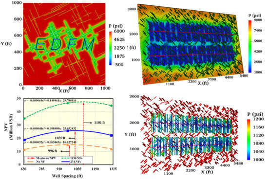
The effect of natural fractures on two shale-gas well performance did not increase linearly with the increasing number of natural fractures. For example, the natural fractures contributed to the incremental gas recovery after 20 years of 22% and 58% for the well spacing of 300 m (984 ft) with a fracture number of 274 and 1196 compared to the no natural fractures case.

(2)

The well interference effect was very dominant at a tight, suboptimal well spacing of 200 m (656 ft), as suggested by the straightforward visualizations of matrix/fracture pressure distributions after 20 years. This effect was also posing severe impacts on the economic performance of the well, especially at a larger number of natural fractures and suboptimal designs of well spacing.

(3)

A greater well spacing was suggested as optimal when the shale-gas reservoir had a larger number of natural fractures. The relative changes of the optimal spacing for 274 natural fractures case and 1196 natural fractures case, when compared to no natural fractures case, were 4.32% and 10.52%.

(4)

Based on maximum NPV estimation, optimal well spacing was technically suggested after appraising multiple scenarios of the number of natural fractures and resolving efficiently myriads of reservoir and fracture uncertainty parameters. However, the company’s final decisions might also consider business financial constraints and objectives out of the scope of this work.

References

1. U.S. Energy Information Administration. Available online: https://www.eia.gov/tools/faqs/faq.php?id=907&t=8 (accessed on 12 March 2020).
2. Jacobs, T. To solve frac hits, unconventional engineering must revolve around them. JPT 2019, 27–31. [Google Scholar] [CrossRef]
3. Rodriguez, A. Inferences of two dynamic processes on recovery factor and well spacing for shale oil reservoir. In Proceedings of the SPE Liquids-Rich Basins Conference-North America, Odessa, TX, USA, 7–8 November 2019. [Google Scholar] [CrossRef]
4. Fiallos Torres, M.X.; Yu, W.; Ganjdanesh, R.; Kerr, E.; Sepehrnoori, K.; Miao, J.; Ambrose, R. Modeling Interwell Interference due to Complex Fracture Hits in Eagle Ford using EDFM. In Proceedings of the International Petroleum Technology Conference, Beijing, China, 26–28 March 2019. [Google Scholar] [CrossRef]
5. Morales, A.; Zhang, K.; Gakhar, K.; Marongiu Porcu, M.; Lee, D.; Shan, D.; Malpani, R.; Pope, T.; Sobernheim, D.; Acock, A. Advanced Modeling of Interwell Fracturing Interference: An Eagle Ford Shale Oil Study-Refracturing. In Proceedings of the SPE Hydraulic Fracturing Technology Conference, The Woodlands, TX, USA, 9–11 February 2016. [Google Scholar] [CrossRef]
6. Xiong, H.; Liu, S.; Feng, F.; Liu, S.; Yue, K. Optimize Completion Design and Well Spacing with the Latest Complex Fracture Modeling & Reservoir Simulation Technologies—A Permian Basin Case Study with Seven Wells. In Proceedings of the SPE Hydraulic Fracturing Technology Conference, The Woodlands, TX, USA, 5–7 February 2019. [Google Scholar] [CrossRef]
7. Tang, J.; Wu, K.; Zuo, L.; Xiao, L.; Sun, S.; Ehlig-Economides, C. Investigation of rupture and slip mechanisms of hydraulic fractures in multiple-layered formations. SPE J. 2019, 24, 2292–2307. [Google Scholar] [CrossRef]
8. Xie, J.; Huang, H.; Ma, H.; Zeng, B.; Tang, J.; Yu, W.; Wu, K. Numerical investigation of effect of natural fractures on hydraulic-fracture propagation in unconventional reservoirs. J. Nat. Gas Sci. Eng. 2018, 54, 143–153. [Google Scholar] [CrossRef]
9. Tang, J.; Wu, K.; Li, Y.; Hu, X.; Liu, Q.; Ehlig-Economides, C. Numerical investigation of the interactions between hydraulic fracture and bedding planes with non-orthogonal approach angle. Eng. Fract. Mech. 2018, 200, 1–16. [Google Scholar] [CrossRef]
10. Balan, H.O.; Gupta, A.; Georgi, D. Optimization of Well and Hydraulic Fracture Spacing for Tight/Shale Gas Reservoirs. In Proceedings of the SPE/AAPG/SEG Unconventional Resources Technology Conference, San Antonio, TX, USA, 1–3 August 2016. [Google Scholar] [CrossRef]
11. Chen, Z.; Liao, X.; Zeng, L. Pressure transient analysis in the child well with complex fracture geometries and fracture hits by a semi-analytical model. J. Pet. Eng. 2020, 191, 107–119. [Google Scholar] [CrossRef]
12. Liang, Y.; Sheng, J.; Hildebrand, J. Dynamic permeability models in dual-porosity system for unconventional reservoirs: Case studies and sensitivity analysis. In Proceedings of the SPE Reservoir Characterization and Simulation Conference and Exhibition, Abu Dhabi, UAE, 8–10 May 2017. [Google Scholar] [CrossRef]
13. Tang, H.; Hasan, R.; Killough, J. Development and application of a fully implicitly coupled wellbore/reservoir simulator to characterize the transient liquid loading in horizontal gas wells. SPE J. 2018, 23, 1615–1629. [Google Scholar] [CrossRef]
14. Abivin, P.; Vidma, K.; Xu, T.; Boumessouer, W.; Bailhy, J.; Ejofodomi, E.; Sharma, A.; Menasria, S.; Mikhailov, M. Data Analytics approach to Frac Hit Characterization in Unconventional Plays: Application to Williston Basin. In Proceedings of the International Petroleum Technology Conference, Dhahran, Saudi Arabia, 13–15 January 2020. [Google Scholar] [CrossRef]
15. Rahman, M.; Sankaran, S.; Molinari, D.; Yuxing, B. Determination of Stimulated Reservoir Volume SRV during Fracturing. A Data-Driven Approach to Improve Field Operations. In Proceedings of the SPE Hydraulic Fracturing Technology Conference, The Woodlands, TX, USA, 4–6 February 2020. [Google Scholar] [CrossRef]
16. McClure, M.; Picone, M.; Fowler, G.; Ratcliff, D.; Kang, C.; Medam, S.; Frantz, J. Nuances and Frequently Asked Questions in Field-Scale Hydraulic Fracture Modeling. In Proceedings of the SPE Hydraulic Fracturing Technology Conference, The Woodlands, TX, USA, 4–6 February 2020. [Google Scholar] [CrossRef]
17. Fowler, G.; McClure, M.; Cipolla, C. A Utica Case Study: The Impact of Permeability Estimates on History Matching, Fracture Length, and Well Spacing. In Proceedings of the SPE Annual Technical Conference and Exhibition, Calgary, AB, Canada, 30 September–2 October 2019. [Google Scholar] [CrossRef]
18. Morales, A.; Holman, R.; Nugent, D.; Wang, J.; Reece, Z.; Madubuike, C.; Flores, S.; Berndt, T.; Nowaczewski, V.; Cook, S.; et al. Case Study: Optimizing Eagle Ford Field Development through a Fully Integrated Workflow. In Proceedings of the SPE Annual Technical Conference and Exhibition, Calgary, AB, Canada, 30 September–2 October 2019. [Google Scholar] [CrossRef]
19. Yu, W.; Sepehrnoori, K. Simulation of gas desorption and geomechanics effects for unconventional gas reservoirs. Fuel 2014, 116, 455–464. [Google Scholar] [CrossRef]
20. Yu, W.; Sepehrnoori, K. Shale Gas and Tight Oil Reservoir Simulation, 1st ed.; Elsevier: Cambridge, MA, USA, 2018; ISBN 978-0-12-813868-7. [Google Scholar]
21. AITwaijri, M.; Xia, Z.; Yu, W.; Qu, L.; Hu, Y.; Xu, Y.; Sepehrnoori, K. Numerical study of complex fracture geometry effect on two-phase performance of shale-gas wells using the fast EDFM method. J. Pet. Sci. Eng. 2018, 164, 603–622. [Google Scholar] [CrossRef]
22. Miao, J.; Yu, W.; Xia, Z.; Zhao, W.; Xu, Y.; Sepehrnoori, K. A simple and fast EDFM method for production simulation in shale reservoirs with complex fracture geometry. In Proceedings of the 2nd International Discrete Fracture Network Engineering Conference, Seattle, WA, USA, 20–22 June 2018. [Google Scholar]
23. Dachanuwattana, S.; Jin, J.; Zuloaga-Molero, P.; Li, X.; Xu, Y.; Sepehrnoori, K.; Yu, W.; Miao, J. Application of proxy-based MCMC and EDFM to history match a Vaca Muerta shale oil well. Fuel 2018, 220, 490–502. [Google Scholar] [CrossRef]
24. Dachanuwattana, S.; Xia, Z.; Yu, W.; Qu, L.; Wang, P.; Liu, W.; Miao, J.; Sepehrnoori, K. Application of proxy-based MCMC and EDFM to history match a shale gas condensate well. J. Pet. Sci. Eng. 2018, 167, 486–497. [Google Scholar] [CrossRef]
25. Yu, W.; Tripoppoom, S.; Sepehrnoori, K.; Miao, J. An automatic history-matching workflow for unconventional reservoirs coupling MCMC and non-intrusive EDFM methods. In Proceedings of the SPE Annual Technical Conference and Exhibition, Dallas, TX, USA, 24–26 September 2018. [Google Scholar] [CrossRef]
26. Tripoppoom, S.; Yu, W.; Sepehrnoori, K.; Miao, J. Application of assisted history matching workflow to shale gas well using EDFM and neural network-Markov Chain Monte Carlo algorithm. In Proceedings of the SPE/AAPG/SEG Unconventional Resources Technology Conference, Denver, CO, USA, 22–24 July 2019. [Google Scholar] [CrossRef]
27. Xu, Y.; Cavalcante Filho, J.S.A.; Yu, W.; Sepehrnoori, K. Discrete-fracture modeling of complex hydraulic-fracture geometries in reservoir simulators. SPE Reserv. Eval. Eng. 2017, 20, 403–422. [Google Scholar] [CrossRef]
28. Xu, Y.; Yu, W.; Sepehrnoori, K. Modeling dynamic behaviors of complex fractures in conventional reservoir simulators. In Proceedings of the SPE/AAPG/SEG Unconventional Resources Technology Conference, Austin, TX, USA, 24–26 July 2017. [Google Scholar] [CrossRef]
29. Moinfar, A.; Varavei, A.; Sepehrnoori, K. Development of an efficient embedded discrete fracture model for 3d compositional reservoir simulation in fractured reservoirs. SPE J. 2014, 19, 289–303. [Google Scholar] [CrossRef] [Green Version]
30. Xu, Y.; Yu, W.; Li, N.; Lolon, E.; Sepehrnoori, K. Modeling well performance in Piceance Basin Niobrara formation using embedded discrete fracture model. In Proceedings of the SPE/AAPG/SEG Unconventional Resources Technology Conference, Houston, TX, USA, 23–25 July 2018. [Google Scholar] [CrossRef]
31. Yu, W.; Miao, J.; Sepehrnoori, K. A revolutionary EDFM method for modeling dynamic behaviors of complex fractures in naturally fractured reservoirs. In Proceedings of the 2nd International Discrete Fracture Network Engineering Conference, Seattle, WA, USA, 20–22 June 2018. [Google Scholar]
32. Yu, W.; Xu, Y.; Weijermars, R.; Wu, K.; Sepehrnoori, K. A numerical model for simulating pressure response of well interference and well performance in tight oil reservoirs with complex-fracture geometries using the fast embedded-discrete-fracture-model method. SPE Reserv. Eval. Eng. 2018, 21, 489–502. [Google Scholar] [CrossRef]
33. Xu, F.; Yu, W.; Li, X.; Miao, J.; Zhao, G.; Sepehrnoori, K.; Li, X.; Jin, J.; Wen, G. A fast EDFM method for production simulation of complex fractures in naturally fractured reservoirs. In Proceedings of the SPE/AAPG Eastern Regional Meeting, Pittsburgh, PA, USA, 7–11 October 2018. [Google Scholar] [CrossRef]
34. Yu, W.; Wu, K.; Zuo, L.; Miao, J.; Sepehrnoori, K. Embedded discrete fracture model assisted study of gas transport mechanisms and drainage area for fractured shale gas reservoirs. In Proceedings of the Unconventional Resources Technology Conference, Denver, CO, USA, 22–24 July 2019. [Google Scholar] [CrossRef]
35. Tripoppoom, S.; Xie, J.; Yong, R.; Wu, J.; Yu, W.; Sepehrnoori, K.; Miao, J.; Chang, C.; Li, N. Investigation of different production performances in shale gas wells using assisted history matching: Hydraulic fractures and reservoir characterization from production data. Fuel 2020, 267, 117097. [Google Scholar] [CrossRef]
36. Yu, W.; Sepehrnoori, K. Optimization of multiple hydraulically fractured horizontal wells in unconventional gas reservoirs. In Proceedings of the SPE Production and Operations Symposium, Oklahoma City, OK, USA, 23–26 March 2013. [Google Scholar] [CrossRef]
Figure 1. The non-intrusive embedded discrete fracture model (EDFM) technology in conjunction with the third-party reservoir simulator to efficiently model fractures in any complex geometry [34]: (a) Sample case with only hydraulic fractures; (b) Sample case with hydraulic (EDFM) and natural fractures.
Energies 13 02853 g001
Figure 2. The workflow for automatic history matching coupling artificial neural network, Markov chain Monte Carlo (MCMC) algorithm, EDFM preprocessor, and reservoir simulator [26].
Energies 13 02853 g002
Figure 3. A field-scale shale gas model, including two horizontal wells with well spacing of 200 m (656 ft) and multi-stage hydraulic fractures and complex natural fractures (NFs): (a) No NF; (b) 274 NFs; (c) 1196 NFs.
Energies 13 02853 g003
Figure 4. Field-scale shale gas model, including two horizontal wells with well spacing of 300 m (984 ft) and multi-stage hydraulic fractures and complex natural fractures: (a) No NF; (b) 274 NFs; (c) 1196 NFs.
Energies 13 02853 g004
Figure 5. A field-scale shale gas model, including two horizontal wells with well spacing of 400 m (1312 ft) and multi-stage hydraulic fractures and complex natural fractures: (a) No NF; (b) 274 NFs; (c) 1196 NFs.
Energies 13 02853 g005
Figure 6. Comparison of flowing BHP and gas and water flow rates between filed data and simulation results: (a) Flowing BHP; (b) Gas flow rate; (c) Water flow rate; (d) Matrix pressure distribution after production history of 511 days.
Energies 13 02853 g006aEnergies 13 02853 g006b
Figure 7. Two-phase relative permeability curves used for the well spacing optimization application.
Energies 13 02853 g007
Figure 8. Flowing bottomhole pressure constraints for 20-year shale gas simulation.
Energies 13 02853 g008
Figure 9. Comparison of well performance with well spacing of 200 m (656 ft): (a) Gas flow rate; (b) Cumulative gas production; (c) Water flow rate; (d) Cumulative water production.
Energies 13 02853 g009
Figure 10. Comparison of well performance with well spacing of 300 m (984 ft): (a) Gas flow rate; (b) Cumulative gas production; (c) Water flow rate; (d) Cumulative water production.
Energies 13 02853 g010
Figure 11. Comparison of well performance with well spacing of 400 m (1312 ft): (a) Gas flow rate; (b) Cumulative gas production; (c) Water flow rate; (d) Cumulative water production.
Energies 13 02853 g011aEnergies 13 02853 g011b
Figure 12. Detailed visualizations of reservoir pressure distributions in both matrix (left column) and fractures (right columns) with two wells, a well spacing of 200 m (656 ft), multi-stage hydraulic fractures, and complex natural fractures: (a) Matrix with no NF; (b) Only hydraulic fractures; (c) Matrix with 274 NFs; (d) Hydraulic fractures and 274 NFs; (e) Matrix with 1196 NFs; (f) Hydraulic fractures and 1196 NFs.
Energies 13 02853 g012
Figure 13. Detailed visualizations of reservoir pressure distributions in both matrix (left column) and fractures (right columns) with two wells, a well spacing of 300 m (984 ft), multi-stage hydraulic fractures, and complex natural fractures: (a) Matrix with no NF; (b) Only hydraulic fractures; (c) Matrix with 274 NFs; (d) Hydraulic fractures and 274 NFs; (e) Matrix with 1196 NFs; (f) Hydraulic fractures and 1196 NFs.
Energies 13 02853 g013
Figure 14. Detailed visualizations of reservoir pressure distributions in both matrix (left column) and fractures (right columns) with two wells, a well spacing of 400 m (1312 ft), multi-stage hydraulic fractures, and complex natural fractures: (a) Matrix with no NF; (b) Only hydraulic fractures; (c) Matrix with 274 NFs; (d) Hydraulic fractures and 274 NFs; (e) Matrix with 1196 NFs; (f) Hydraulic fractures and 1196 NFs.
Energies 13 02853 g014aEnergies 13 02853 g014b
Figure 15. Calculated net present value (NPV) associated with all nine scenarios, along with interpolated optimal well spacing, maximum NPV, and the curve-fitting equations of well spacing-NPV relationship.
Energies 13 02853 g015