Effect of Fins on the Internal Flow Characteristics in the Draft Tube of a Francis Turbine Model

Abstract

Undesirable flow phenomena in Francis turbines are caused by pressure fluctuations induced under conditions of low flow rate; the resulting vortex ropes with precession in the draft tube (DT) can degrade performance and increase the instability of turbine operations. To suppress these DT flow instabilities, flow deflectors, grooves, or other structures are often added to the DT into which air or water is injected. This preliminary study investigates the effects of anti-cavity fins on the suppression of vortex ropes in DTs without air injection. Unsteady-state Reynolds-averaged Navier–Stokes analyses were conducted using a scale-adaptive simulation shear stress transport turbulence model to observe the unsteady internal flow and pressure characteristics by applying anti-cavity fins in the DT of a Francis turbine model. A vortex rope with precession was observed in the DT under conditions of low flow rate, and the anti-cavity fins were confirmed to affect the mitigation of the vortex rope. Moreover, at the low flow rate conditions under which the vortex rope developed, the application of anti-cavity fins was confirmed to reduce the maximum unsteady pressure.

1. Introduction

Since hydropower technology has a low impact on the natural environment, there is significant potential for its efficient application in power generation. Traditionally, hydroelectric power generated by hydro turbines has been used to provide electrical energy during times of peak load. However, as solar and wind power technologies with intermittent power generation have recently been developed and added to the grid, the requirement for large and flexible energy adjustments for these instabilities has increased. Consequently, hydro turbines are used over range with off-design operating conditions to provide a base load to maintain a constant frequency and provide a stable power supply. However, because of variations in operating conditions, existing hydro turbines must operate with significant fluctuations in flow rates; this results in both the failure of the turbine systems and a reduction in service lifespan. Particularly, those operations under conditions of low flow rates generate a complicated flow in the draft tube (DT) as a vortex rope, resulting in severe noise and vibration [1,2,3].

Francis turbines exhibit the undesirable phenomenon of a vortex rope with precession, which induces pressure fluctuations in the DT under low flow rate conditions. A pressure fluctuation frequency close to the natural frequency of the system causes a resonance that seriously undermines the stability of the turbine system [4,5].

To examine these influences on turbine systems, many studies have attempted to investigate the flow mechanisms and characteristics of the vortex rope in the DT. Susan-Resiga et al. [6] used an axisymmetric flow model to numerically study a methodology for analyzing the swirling flows of a vortex rope. This axisymmetric flow solver provides a circumferential averaged flow field. Nicolet et al. [7] conducted an experimental investigation of pressure fluctuations with vortex ropes at the upper-part load; they used high-speed camera visualization with synchronized measurement of pressure fluctuations in a Francis turbine model with high specific speed. Zuo et al. [8] used a Francis turbine model to assess the stability of a vortex rope in a DT under different operating conditions; via unsteady simulations, they observed the relationships between the induced hydraulic instabilities and the characteristics of the vortex rope. Favrel et al. [5] explored the influence of flow rate on the structure and parameters of vortex ropes. The intensity of the excitation source was observed for the vortex rope dynamics using PIV measurements in a Francis turbine operating at part load.

To suppress the flow instabilities associated with the vortex rope in the DT, several previous studies have modified the tube’s internal flow; modifications have included injecting air or water or adding internal flow deflectors or grooves to the DT’s cone. Aeration and water injection are well-established control methods for suppressing pressure fluctuations within the DT. These injections work to decrease the turbulence intensity of the swirl flow by increasing the momentum of axial flow in the central region, thereby stabilizing the operation of the hydro turbine system [9].

Altimemy et al. [9] conducted a large eddy simulation at the design and partial loading stages of the Francis turbine to examine the influence of water injection on pressure fluctuations and flow behavior in the DT. Susan-Resiga et al. [10] performed an investigation to mitigate the severe flow fluctuations induced by the vortex rope in a Francis turbine operating at part load by numerically determining a method for injecting a water jet from the crown tip of the runner. WF et al. [11] applied numerical analyses to reduce pressure fluctuations by simulating the unsteady flow in the DT of a Francis turbine and incorporating air and water injections and flow deflectors within the DT. Feng et al. [4] conducted a numerical analysis to decrease the pressure fluctuations caused by the vortex rope in the DT of a Francis turbine by applying extended runner cones, damping gates, and flow deflectors in the DT. Anup et al. [12] numerically calculated the four different depths of the J-Grooves in the DT to minimize vortex rope characteristics and flow instabilities. Chen and Choi [13] used both experimental and numerical approaches to investigate the effects of the J-Groove on the DT wall in suppressing cavitation in the DT of a Francis turbine.

Anti-cavity fins with air injection are often applied to aid the suppression and minimization of the vortex rope by the DT wall. However, the effects of DT anti-cavity fins on the internal flow and the unsteady pressure characteristics without air injection have not been systematically elucidated under low flow rate conditions in a Francis turbine.

Therefore, this study preliminarily investigates the effects of anti-cavity fins for suppressing the vortex characteristics in the DT in a Francis turbine. Anti-cavity fins without air injection were applied in the DT of a Francis turbine model, and the internal flow and unsteady pressure characteristics at low flow rates were assessed. The investigation performs unsteady-state Reynolds-averaged Navier–Stokes (RANS) equations using a scale-adaptive simulation shear stress transport (SAS-SST) turbulence model to observe the unsteady internal flow and pressure fluctuation characteristics in the presence of vortex rope and anti-cavity fins under conditions of low flow rate. The research compares the magnitudes and locations of the vortex rope via the application of anti-cavity fins under low flow rate conditions, and the results are discussed concerning the effects of the fins. Furthermore, to investigate the unsteady pressure fluctuations induced by the vortex ropes with precession, pressure measurement points were applied on the wall of the DT to analyze the unsteady flow.

2. Francis Turbine Model and Anti-Cavity Fins

This study conducted three-dimensional (3-D) unsteady-state numerical analyses of a Francis turbine model with a specific speed of 270-class [m, kW, min⁻¹]. The model’s specific speed was calculated using Equation (1). Figure 1 presents a 3-D model of the DT of the Francis turbine model, which shows the locations of the anti-cavity fins. The fins comprised two short fins and two long fins; the two short fins were the same length (0.7 D₂) and were arranged to face each other, whereas the two long fins also faced each other but were of different lengths (1.09 and 1.3 D₂, respectively). Here, D₂ is defined as the outlet diameter of the runner. The anti-cavity fins with the air injection outlet (the dotted red circles in Figure 1a) were located at 0.2 D₂ on the wall of the DT’s cone, and the air injection outlet protruded from the anti-cavity fins. This study considered the shapes of the air injection outlets in the analysis domain to accurately reflect the shape of the DT without considering the effects of the air injection. The specifications of the Francis turbine model are listed in

Table 1. Francis turbine model specifications.

Specification	Value
Speed factor, nED (–)	0.48
Discharge coefficient, QED (–)	0.33
Energy coefficient, EnD (–)	4.35
Diameter of runner outlet, D2 (m)	0.35
Number of runner blades	12
Number of stay vanes	20
Number of guide vanes	20

and include the speed factor, discharge factor, and energy coefficient. These coefficients and factors are applied along with Equations (2)–(4) and are defined by IEC Standard 60193 [14].

$$N_s=\frac{N\sqrt{P}}{H^{\frac{5}{4}}}$$

(1)

$$n_{ED}=\frac{nD}{\sqrt{gH}}$$

(2)

$$Q_{ED}=\frac{Q}{D^2{E}^{0.5}}$$

(3)

$$E_{nD}=\frac{gH}{n^2{D}^2}$$

(4)

3. Numerical Analysis Methods

This study used ANSYS CFX-19.1 commercial software [15] to analyze the 3-D internal flow field of the Francis turbine model in terms of the unsteady-state calculations. The numerical grids for the runner and vane components were generated using the software’s TurboGrid function, whereas the numerical grids of the spiral casing (SC) and DT were produced using the ANSYS Meshing and ICEM-CFD functions. The boundary conditions for the numerical analysis were set using CFD-Pre, and to solve the governing equations and to conduct the post-processing of the results, CFX-Solver and CFX-Post were used, respectively. The unsteady-state RANS equations for the incompressible flow behavior of the Francis turbine model were calculated using governing equations (Equations (5) and (6)), which were discretized via the finite volume method.

$$\frac{\partial \rho }{\partial t}=\frac{\partial \left(\rho u_i\right)}{\partial x_i}=0$$

(5)

$$\frac{\partial \left(\rho u_i\right)}{\partial t}+\frac{\partial \left(\rho u_i{u}_j\right)}{\partial x_j}=-\frac{\partial p}{\partial x_i}+\frac{\partial }{\partial x_j}\left(\mu \frac{\partial u_i}{\partial x_j}\right)+\frac{\partial {\tau }_{ij}}{\partial x_j}$$

(6)

where ${\tau }_{ij}=-\rho \overline{u_i{u}_j}$ is known as the Reynolds stress. To ensure the physical boundaries, the discretizations of the high-resolution and second-order backward Euler schemes were solved for the advection and transient schemes.

The numerical grids of the Francis turbine model are presented in Figure 2. The computational domains of the SC and DT were constructed using tetrahedral-type grids, whereas hexahedral-type grids were applied for the construction of the computational domains of the stay vanes (SVs), guide vanes (GVs), and runner blades. In the runner domain, O-type grids were used on the surface of the runner blade, and the y+ value for the first runner grid point was kept below five. The grid convergence index method was applied to select the optimum grids among the three observed grids to estimate the numerical uncertainty due to discretization error [16,17,18]. Figure 3 presents a comparison between the efficiency and flow rates for the three observed numerical grids. The $GC{I}_{fine}^{21}$ values of the efficiency and flow rates were calculated to be about 0.0022 and 0.0458, respectively, for the optimum grids of 14.74 × 10⁶, as shown in

Table 2. Calculation of discretization error for the Francis turbine model.

	ϕ = Efficiency	ϕ = Flow Rate
N1, N2, N3	14.74 × 106, 7.05 × 106, 3.59 × 106
r21	1.28
r32	1.25
ϕ1	1	1
ϕ2	0.9952	0.9841
ϕ3	0.9808	0.9618
p	5.20	1.51
$GC{I}_{fine}^{21}$	0.0022	0.0458

. These values were subsequently chosen for the numerical analyses [19].

The boundary conditions for numerical analyses are listed in

Table 3. Boundary conditions of the Francis turbine model.

Boundary Conditions
Working fluid	Water and vapor at 25 °C
Cavitation model	Rayleigh-Plesset
Inlet	Total pressure (Level of upper reservoir)
Outlet	Static pressure (Level of lower reservoir)
Turbulence model	SAS-SST model
Interface condition	Transient rotor-stator
Unsteady calculation conditions	Total time: 8 revolutions of runner Time step: 1.5° of runner Loops coefficient: 5

. The working fluids (water and water vapor) were set at 25 °C to consider the cavitation phenomena using the Rayleigh–Plesset equation, which describes the growth and collapse of vapor bubbles in a liquid as a homogeneous model [20]. Here, the mean diameter of the cavitation bubble was established as 2.0 × 10⁻⁶ m, and the water saturation pressure was set to 3169.9 Pa. The values for area-averaged total pressure and static pressure were established with consideration of the water levels of the upper and lower reservoirs at the inlet and outlet, respectively. To accurately calculate the influence of the flow separation phenomena, the SAS-SST turbulence model was employed, which provides the scale resolving simulation mode to the unsteady SST turbulence model. This is developed by including the von Karman length scale into the turbulence scale equation [21,22]. The transient rotor–stator condition was used to connect the interface between the rotating and stationary domains. Unsteady-state numerical analyses were performed at intervals of 1.5° over a total of eight revolutions of the runner at a time step of 0.0002272 s and a total time of 0.4364 s. To improve the convergence, the coefficient for the number of loops was set at 5. Finally, to investigate the time-averaged values and to avoid initial numerical noise, the values for the period of the runner’s last three revolutions were averaged after a total of five revolutions.

Figure 4 presents the pressure measurement points in the Francis turbine model. To investigate the unsteady pressure characteristics caused by the vortex and internal flow phenomena, these measurement points were applied at regular intervals of 0.1 D₂ on the DT wall. The pressure measurement points (p1–p4 in Figure 4) were located at the same height on the DT wall.

4. Results and Discussion

4.1. Validation of the Numerical Analysis Results

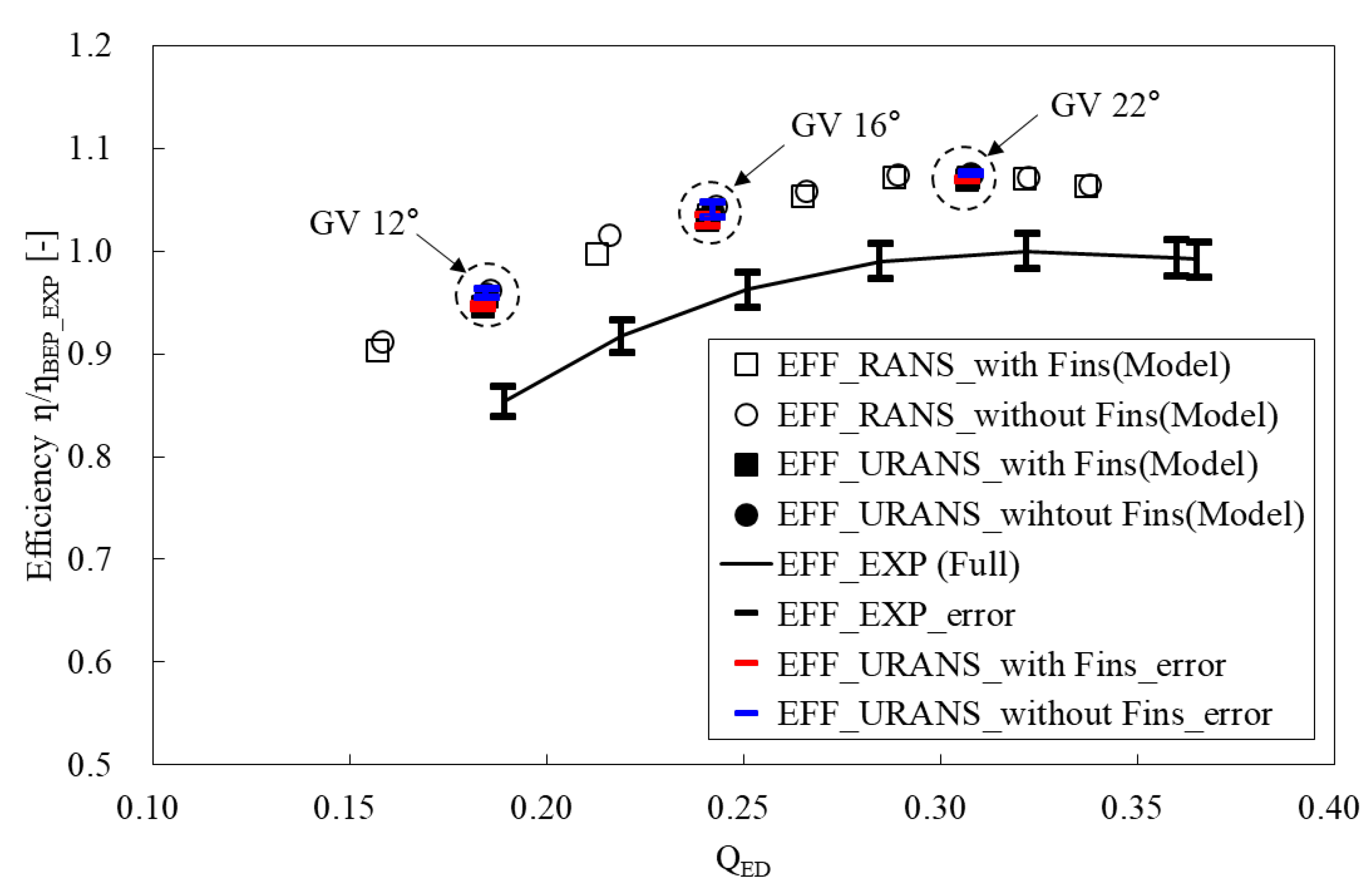
To validate the unsteady-state numerical analysis results of the Francis turbine model, this study compared the results of the steady and unsteady-state RANS equations with the experimental results of the full-scale Francis turbine, as shown in Figure 5. The efficiencies were normalized by the maximum value of experimental efficiency. In the unsteady-state numerical analyses, two low flow rate conditions with GV angles at 16° and 12° were selected as the observed low flow rate conditions based on the best efficiency point (BEP) with a GV at 22°. The full-scale Francis turbine investigations were conducted using the pressure–time method with a measurement error of ±1.74% [23]. To compare the efficiencies between the model and the full-scale Francis turbine, the scale-up conversion of the hydraulic efficiency defined by IEC Standard 60193 was applied to the results of the Francis turbine model’s analysis for both steady and unsteady-state RANS [14]. Equations (7)–(9) were applied as the formulae for scaling up the hydraulic efficiency, whereas Equation (7) was considered as the loss efficiency due to the model’s geometrical scale. The equations of loss efficiency were calculated as a function of the Reynolds number along with Equations (8) and (9), as follows:

$${\eta }_P={\eta }_M+{\left(\Delta \eta \right)}_{M \to P}$$

(7)

$${\left(\Delta \eta \right)}_{M \to P}={\delta }_{ref}\left[{\left(\frac{R{e}_{ref}}{R{e}_M}\right)}^{0.16}-{\left(\frac{R{e}_{ref}}{R{e}_P}\right)}^{0.16}\right]$$

(8)

$${\delta }_{ref}=\frac{1-{\eta }_{opt.M}}{{\left(\frac{R{e}_{ref}}{R{e}_{opt.M}}\right)}^{0.16}-\frac{1-V_{ref}}{V_{ref}}}$$

(9)

where the subscripts of M and P indicate the model and the full-scale Francis turbine, respectively, and $R{e}_{ref}$ = 7 × 10⁶, $V_{ref}$ = 0.7 are the reference values of a radial turbine defined by IEC Standard 60193 [14]. The results of the unsteady-state numerical analyses were averaged during the last three revolutions of the runner to enable an efficiency comparison.

The comparisons between the experimental and the conversed numerical results demonstrate a slight variation for each efficiency. However, the tendencies of the conversed efficiencies of the numerical analyses were similar to those exhibited by the experimental efficiencies; these variations in efficiency comparisons can be interpreted as the neglect of the mechanical loss and the surface roughness in the numerical analyses. Consequently, this study considered the numerical analysis results for the Francis turbine model to be valid. However, the addition of anti-cavity fins decreased the efficiencies across the entire range of observed flow rates. Particularly, in the unsteady-state analyses, the efficiencies of the GVs at 22°, 16°, and 12° decreased by 0.5%, 0.8%, and 1.0%, respectively, depending on the anti-cavity fins applied.

4.2. Internal Flow Characteristics Relative to the Anti-Cavity Fins in the Draft Tube

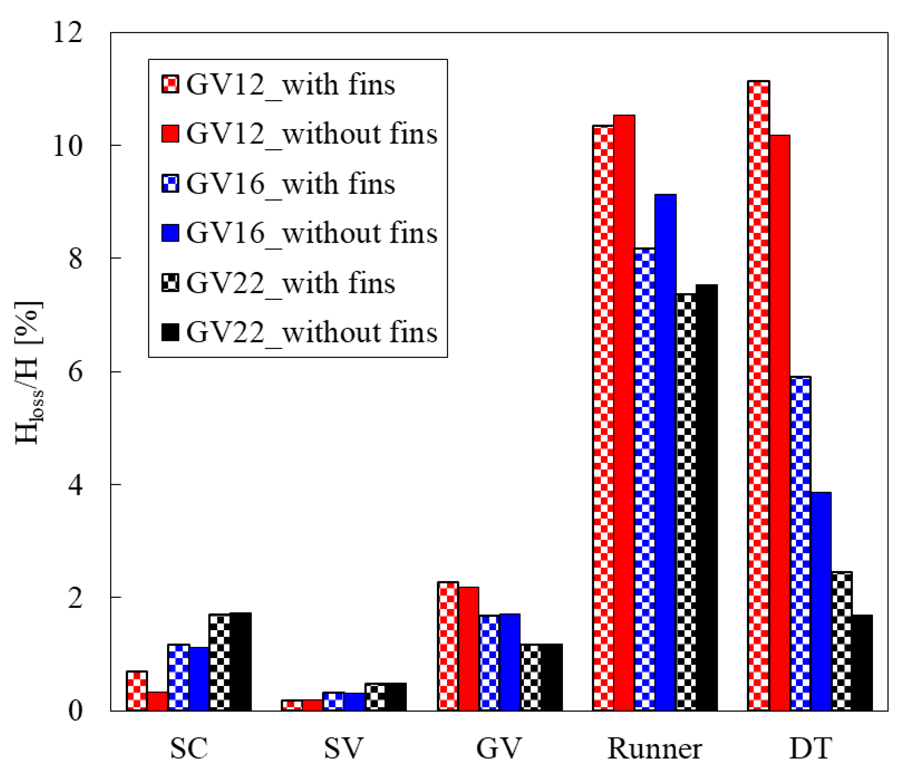
This study investigated the performance characteristics concerning the anti-cavity fins in the DT and the flow rate conditions by calculating the head losses of the main components of the Francis turbine model, as presented in Figure 6. The model’s head losses were calculated using Equation (10) for the SC, SV, GV, and DT, whereas Equation (11) was applied to calculate the head loss of the runner [24].

$$H_{loss}=\frac{\Delta p_{total}}{\rho g}$$

(10)

$$H_{loss runner}=\frac{\Delta p_{total}-\frac{T\omega }{Q}}{\rho g}$$

(11)

Here, H_loss represents the value of loss by a head, ∆p_total is the total pressure difference through each component, which was calculated with time-averaged total pressure in this study, ρ is the water density, and g is the acceleration due to gravity. In the H_{loss runner}, T is the torque of the runner, which was measured by the force caused by a rotating axis, and ω is the angular velocity.

Similar head loss distributions were exhibited from the SC to the GV regions both with and without anti-cavity fins, whereas the inclusion of anti-cavity fins caused slight decreases in the runner’s head losses. However, the application of anti-cavity fins in the DT increased the head losses; these losses were comparatively greater than the decreases in head loss in the runner region. In particular, the difference in head loss in the DT region due to the addition of anti-cavity fins was about 2.0% with a GV at 16°, which was relatively the highest under observed conditions of flow rate.

To investigate the qualitative effect of anti-cavity fins to the magnitude of vortex rope in DT according to the flow rate conditions, Figure 7, Figure 8 and Figure 9 show the vortex rope in the DT by the iso-surface distributions of pressure during the last revolution of the runner for investigating the internal flow structures of GVs at 22°, 16°, and 12°. The iso-surface of pressure was determined as the relative water saturation pressure considering the water level of the lower reservoir. As Figure 7b reveals, with a GV at 22°, the vortex rope in the low-pressure region was not generated in the DT without anti-cavity fins. 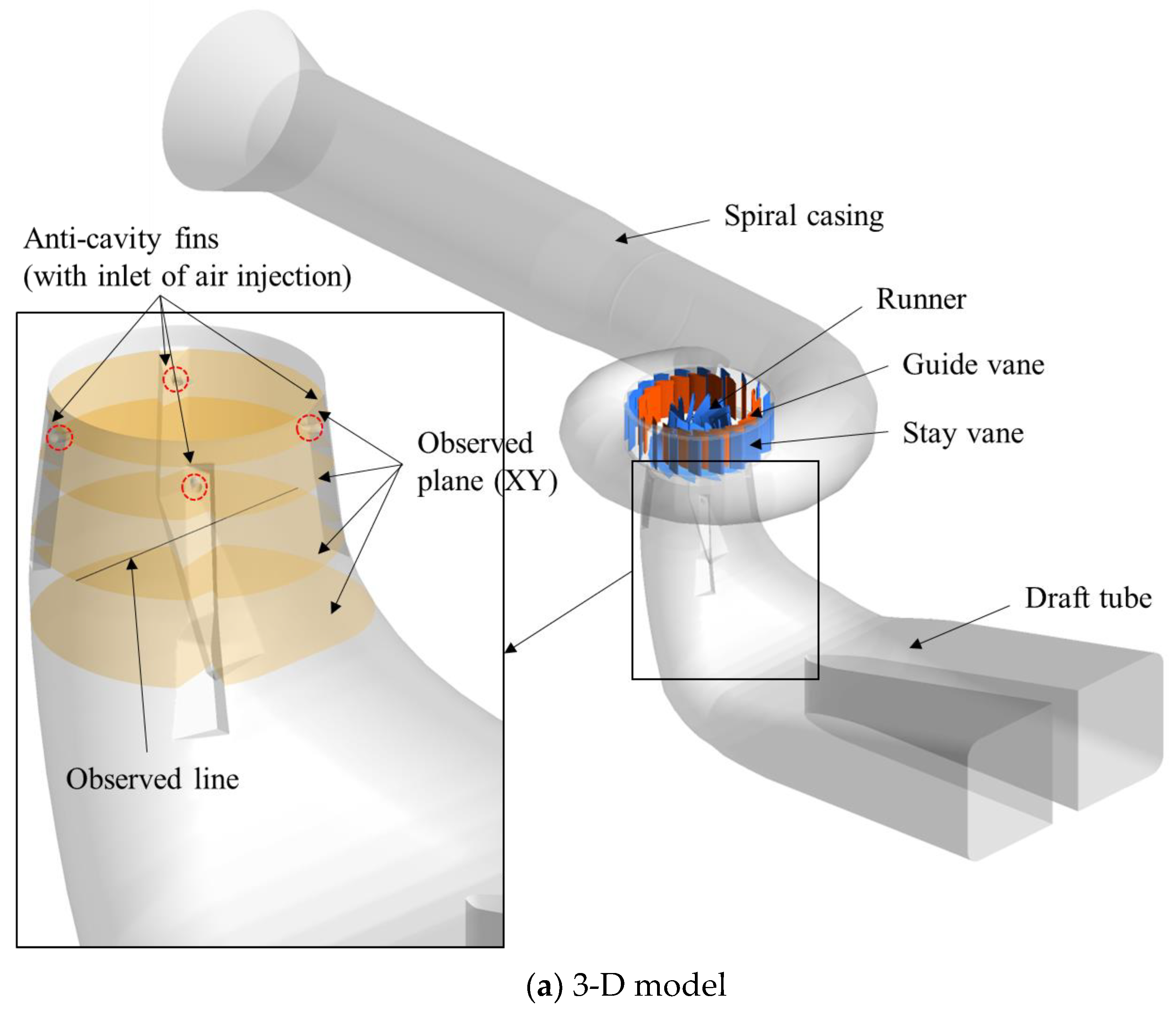However, as can be seen in Figure 7a, the application of anti-cavity fins produced low-pressure regions in the DT. Due to the protrusion of the air injection outlets on the anti-cavity fins, the low-pressure regions occurred on the anti-cavity fins near the inlet of the DT (as detailed in Figure 1). Therefore, it is believed that inducing flow resistance at the sites of the air injection outlets generated the low-pressure regions. 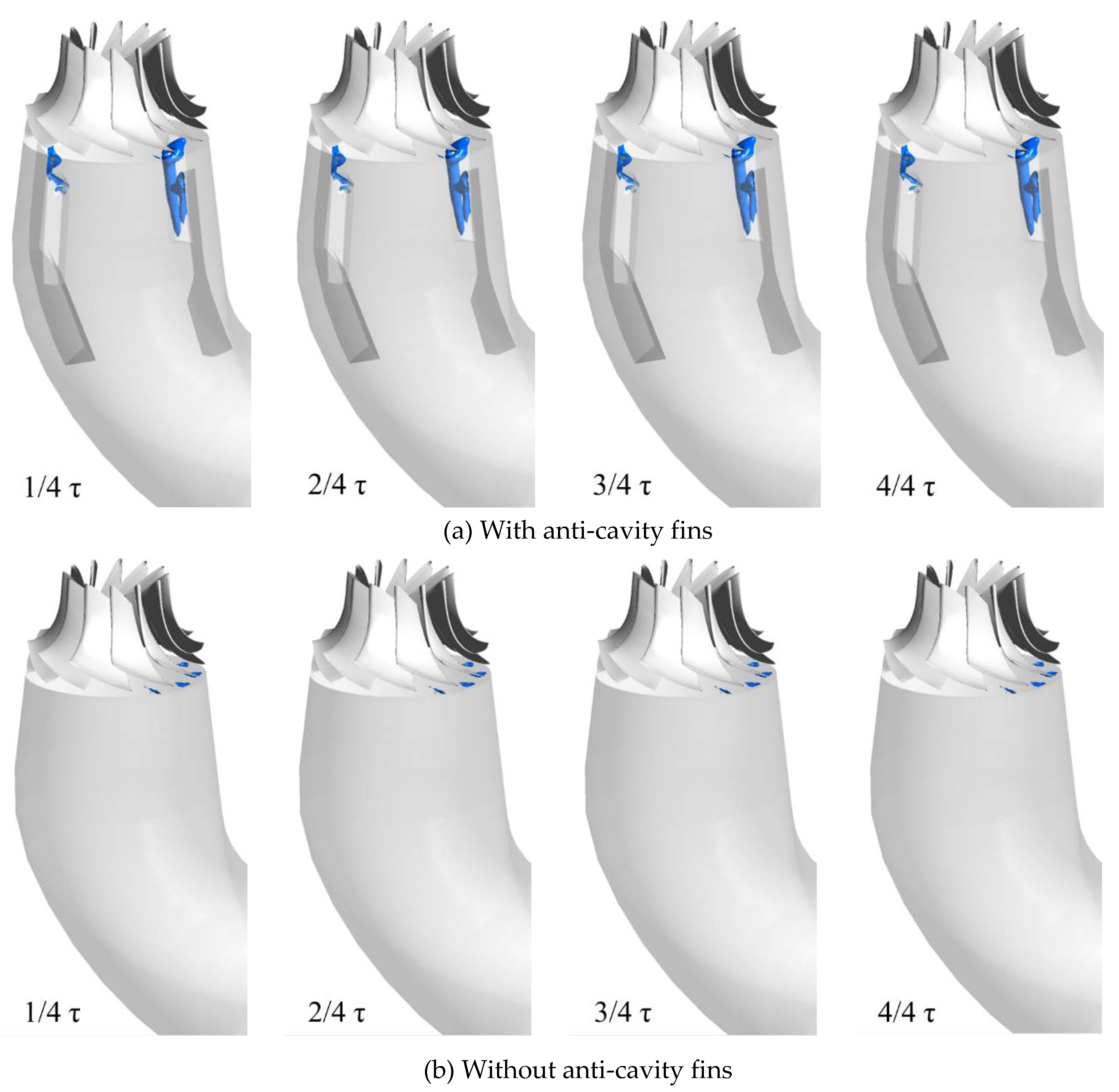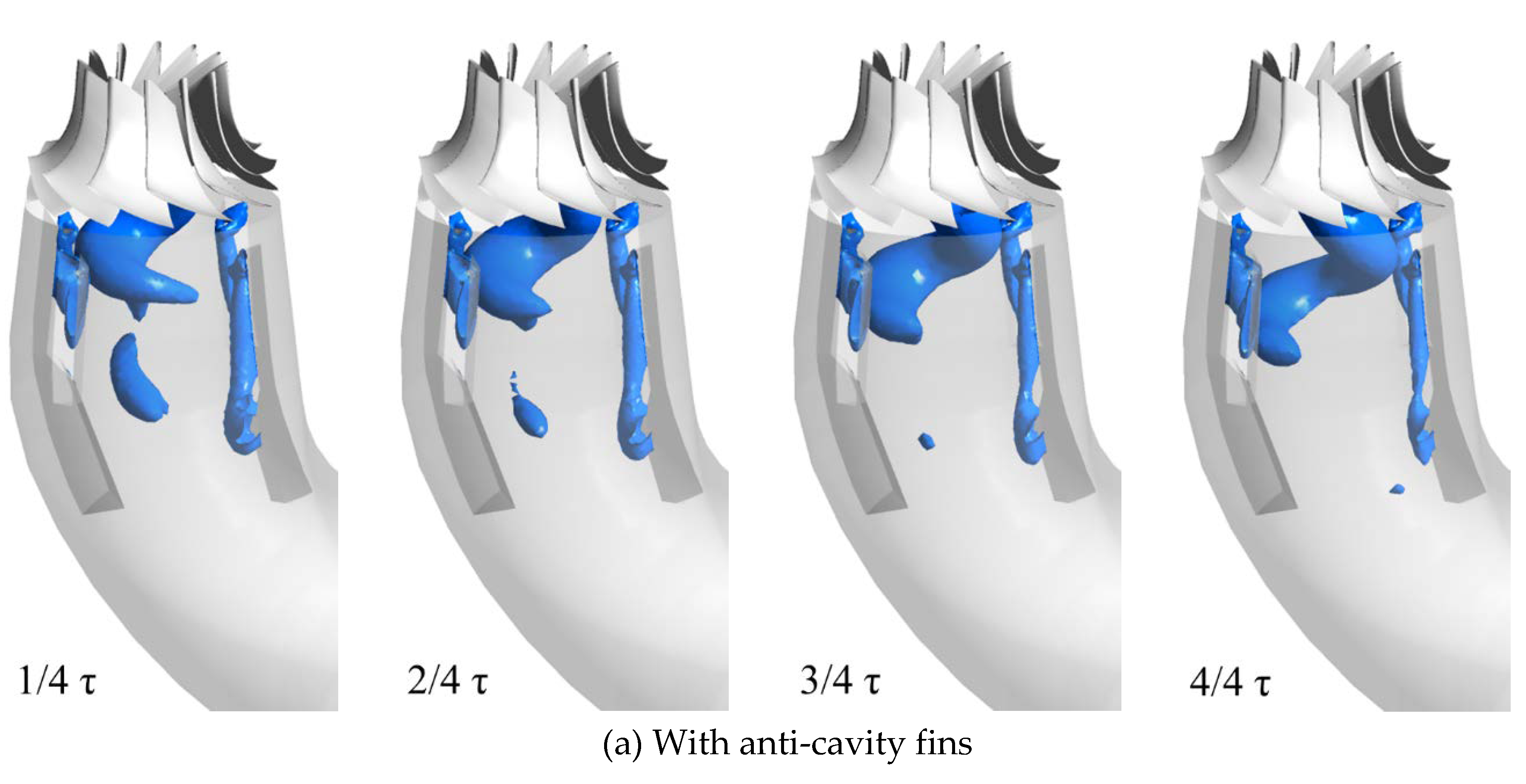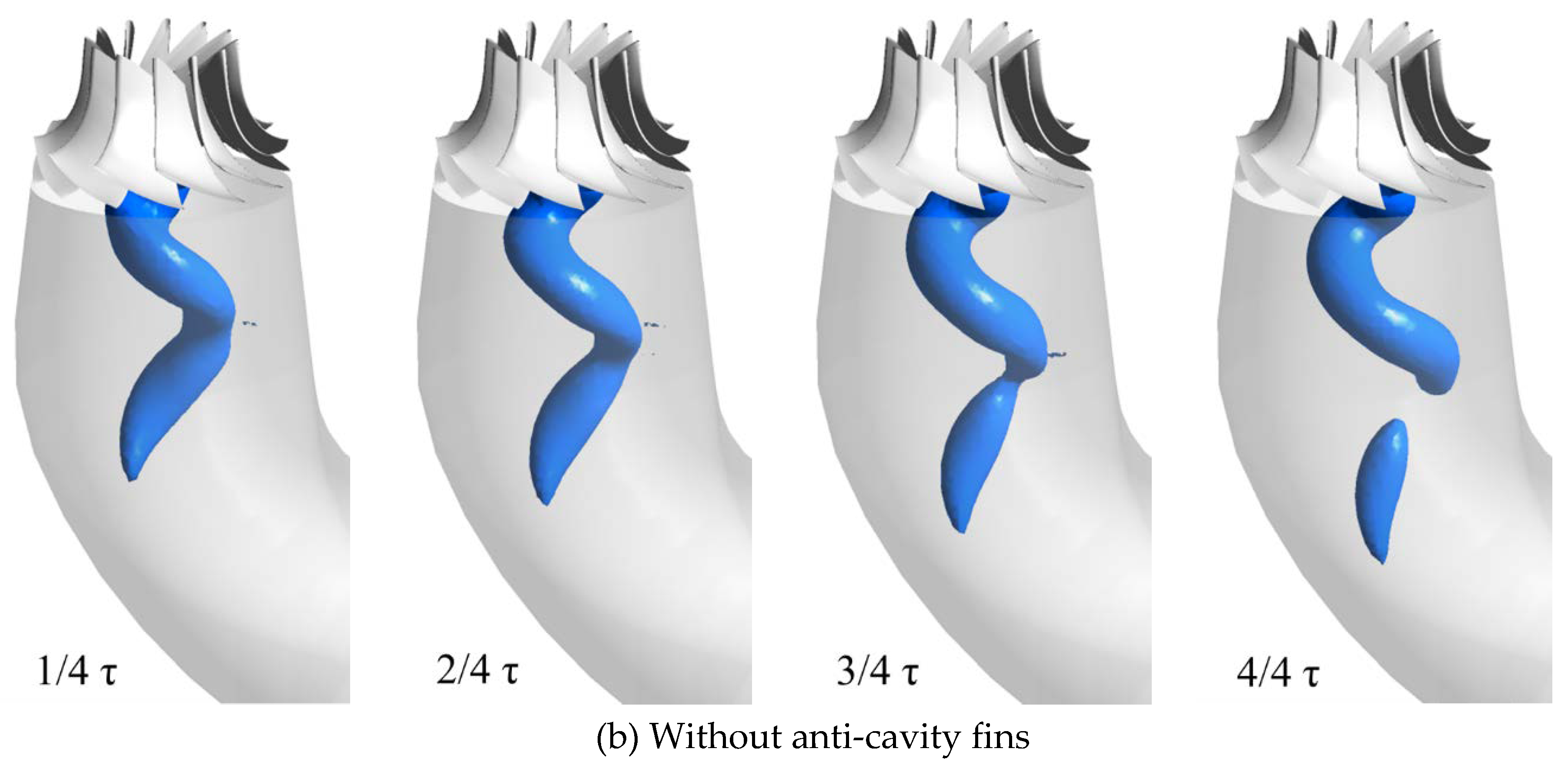Figure 8 shows that the vortex rope was clearly developed in the DT with a GV at 16° (0.78 Q_BEP). The application of anti-cavity fins in the DT significantly decreased the vertical length of the vortex rope. Additionally, the low-pressure regions were found to occur near the anti-cavity fins. Figure 9 shows the condition of the GV at 12° (0.59 Q_BEP). Here, and similar to that shown in Figure 7a, without the addition of anti-cavity fins, no low-pressure regions in the DT were generated. However, Figure 9a reveals that the low-pressure regions were developed on the anti-cavity fins rather than those with a GV at 22° as the difference under both conditions of GV. In this way, the anti-cavity fins in the DT show the effect of reducing the vertical length of the vortex rope, but the shape itself, such as in the air injection outlets, acts as the factor that induces the low-pressure regions and impedes the flow in the DT. It can be regarded as the cause of the increased head loss by application of the anti-cavity fins in the DT, as shown in Figure 6.

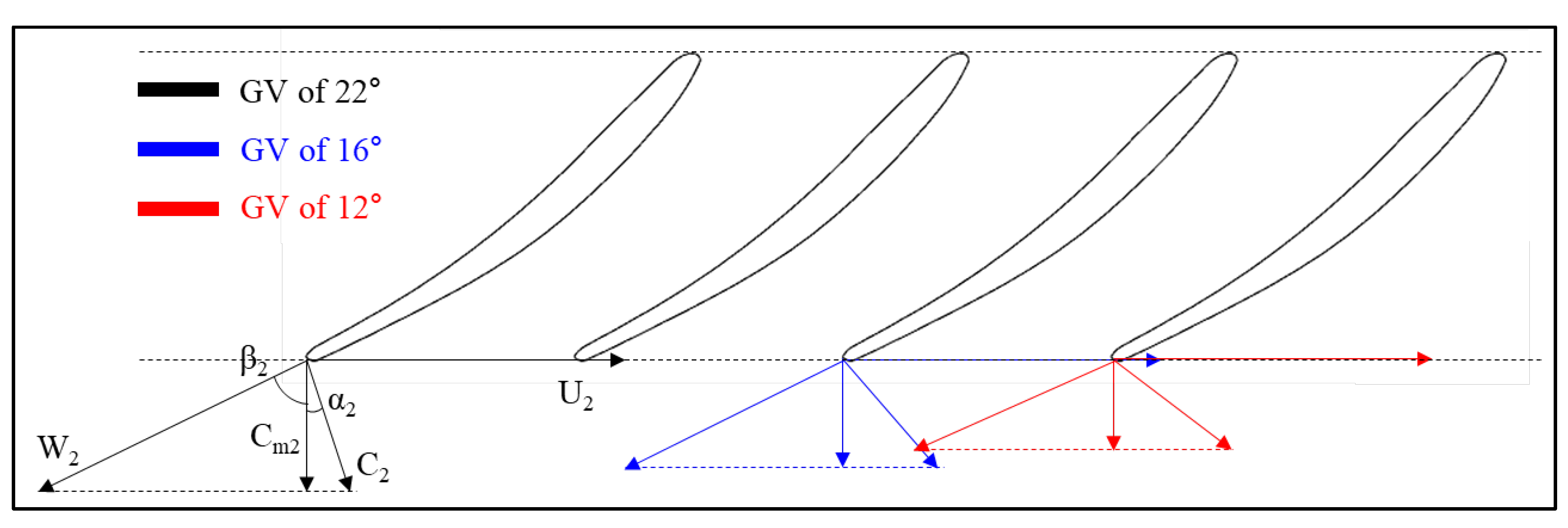
To observe the flow phenomena in the DT according to the flow rate, this study compared the velocity triangles at the runner outlet with GVs at 22°, 16°, and 12°, as illustrated in Figure 10. As the meridional velocity, C_m, decreased, the absolute flow angle, α₂, gradually increased as the GV angle decreased. Thus, in the absolute velocity component, C₂, the radial velocity component increased as the α₂ also increased. The increase in the swirl strength of the flow and the generation of both the complicated flow and the vortex rope in the DT can be due to the increase in the radial velocity component at the outlet of the runner under conditions of low flow rate.

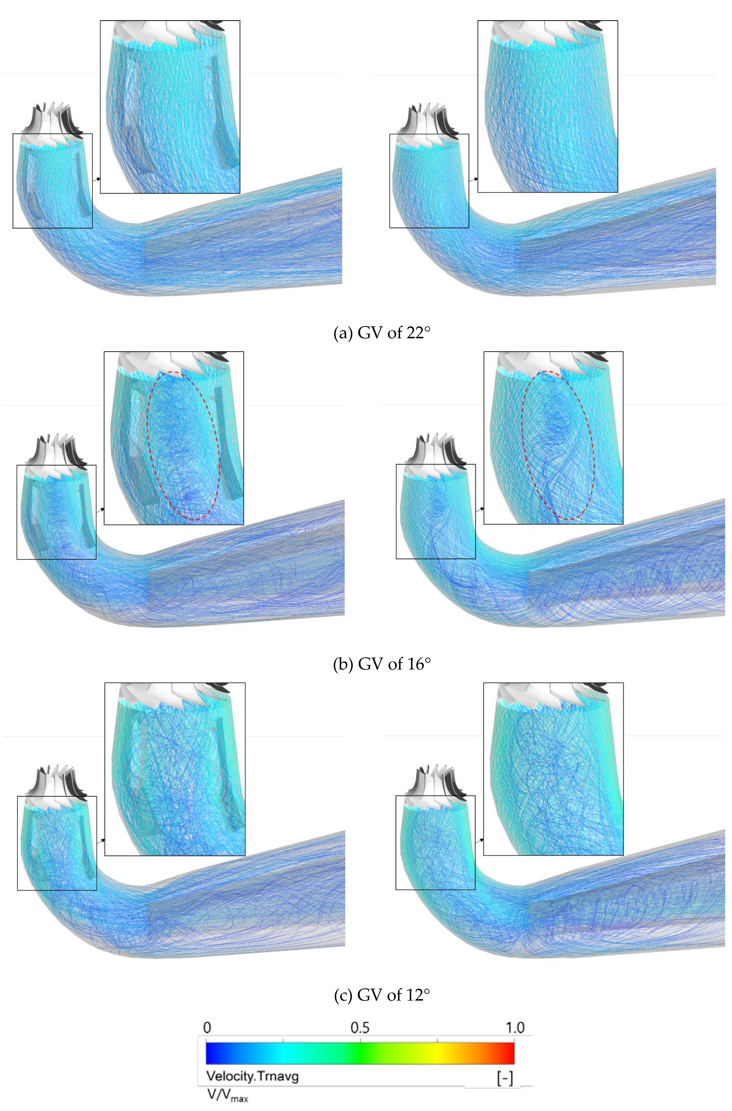
The streamline distributions of the time-averaged (Trnavg) velocity in the DT both with and without the anti-cavity fins are presented in Figure 11 for GVs at 22°, 16°, and 12°. The flow phenomena in the DT are shown with the associated complicated flow at low flow rates as confirmed by the flow characteristics at the runner outlet in the velocity triangles in Figure 10. Figure 11b presents the complicated flow with precession in the DT with a GV at 16°. As Figure 8 shows, the internal flow makes it possible to confirm the cause of the development of the vortex rope and the low-pressure region near the anti-cavity fins in the DT. Figure 11c presents a very complicated internal flow pattern without precession due to the increased radial velocity component with a GV at 12°. These flow characteristics can be confirmed as the reason for the development of the low-pressure regions on the anti-cavity fins, as shown in Figure 9a.

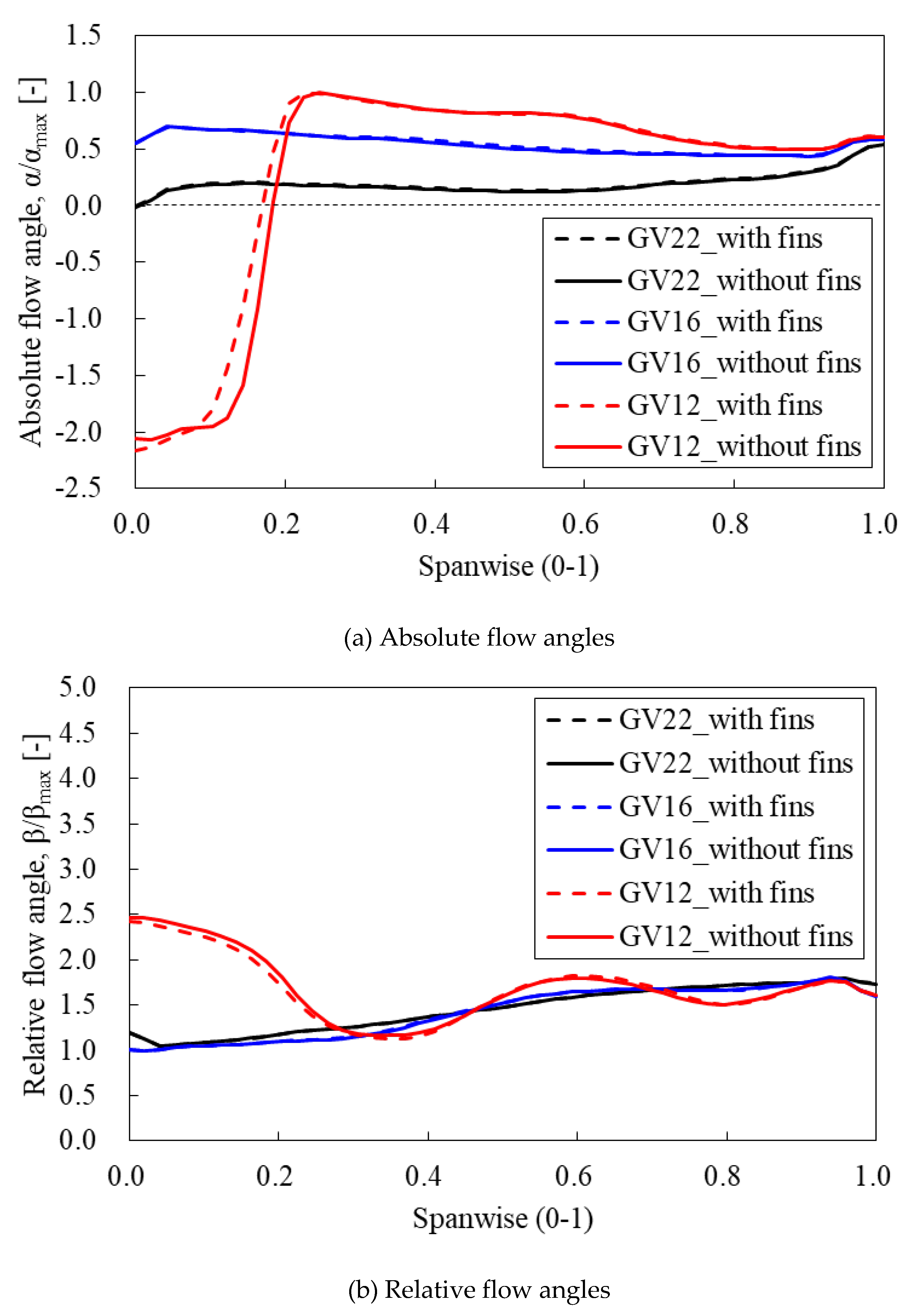
The angle distributions of the absolute and relative flows at the runner outlet along the spanwise direction from hub (0) to shroud (1) with GVs at 22°, 16°, and 12° are presented in Figure 12. The observed flow angles are normalized by the value of each maximum flow angle. The GVs at 22° and 16° demonstrated similar distributions of flow angles both with and without anti-cavity fins, whereas the GV at 12° produced a slight difference in flow angle distributions. This is due to the complicated internal flow characteristics induced by low flow rate conditions. The absolute flow angle distributions at the 22° GV are close to 0, and the absolute flow angles increase as the flow rates decrease. Additionally, compared with the other GV conditions, the contrasting trends are exhibited only at the GV at 12° near the spanwise range of 0–0.2. Similarly, the GV at 12° also demonstrates different tendency characteristics in relative flow angle distribution due to the complicated internal flow, as shown in Figure 12b, although the relative flow angle and the angle of the runner blade outlet generally appear similar.

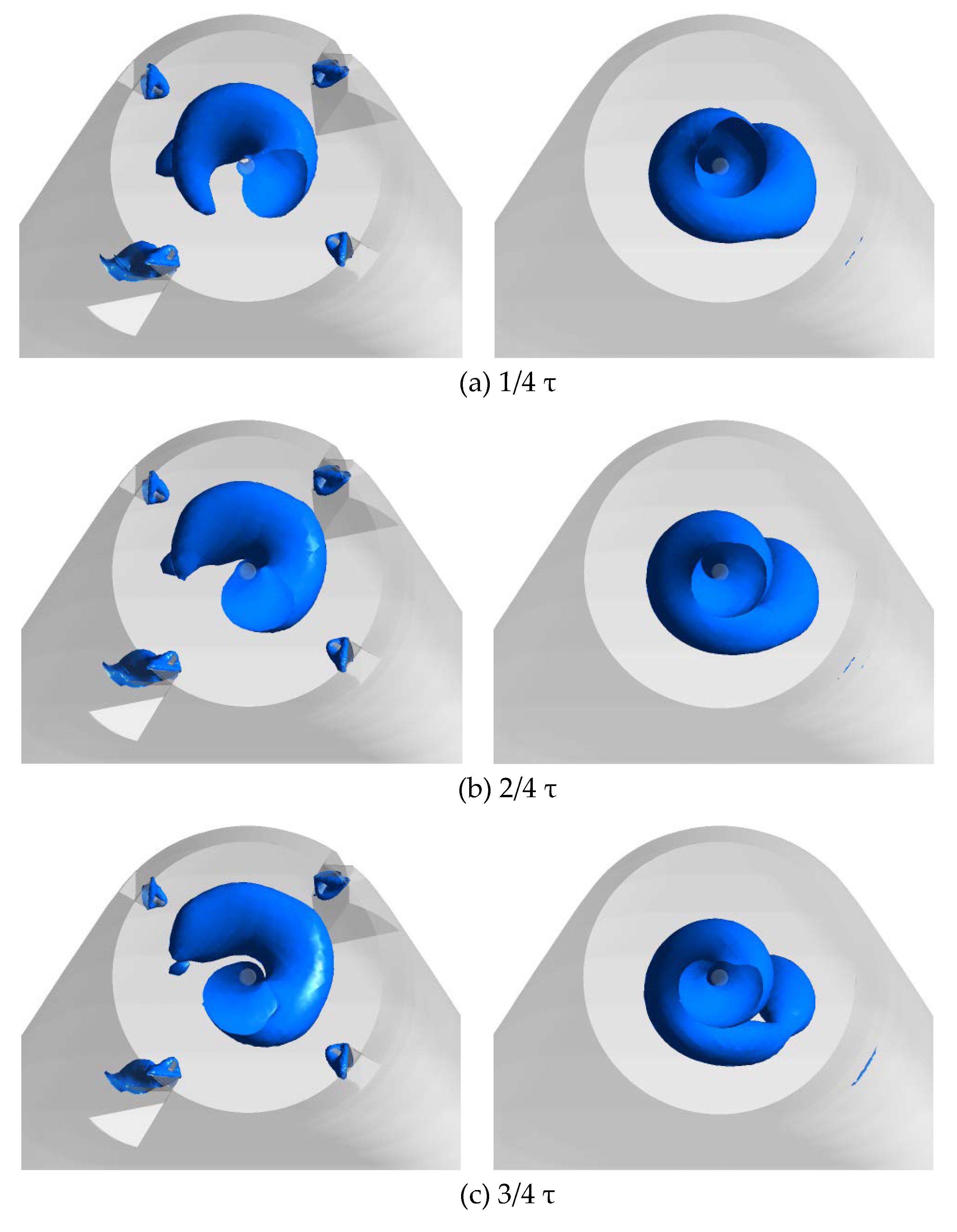
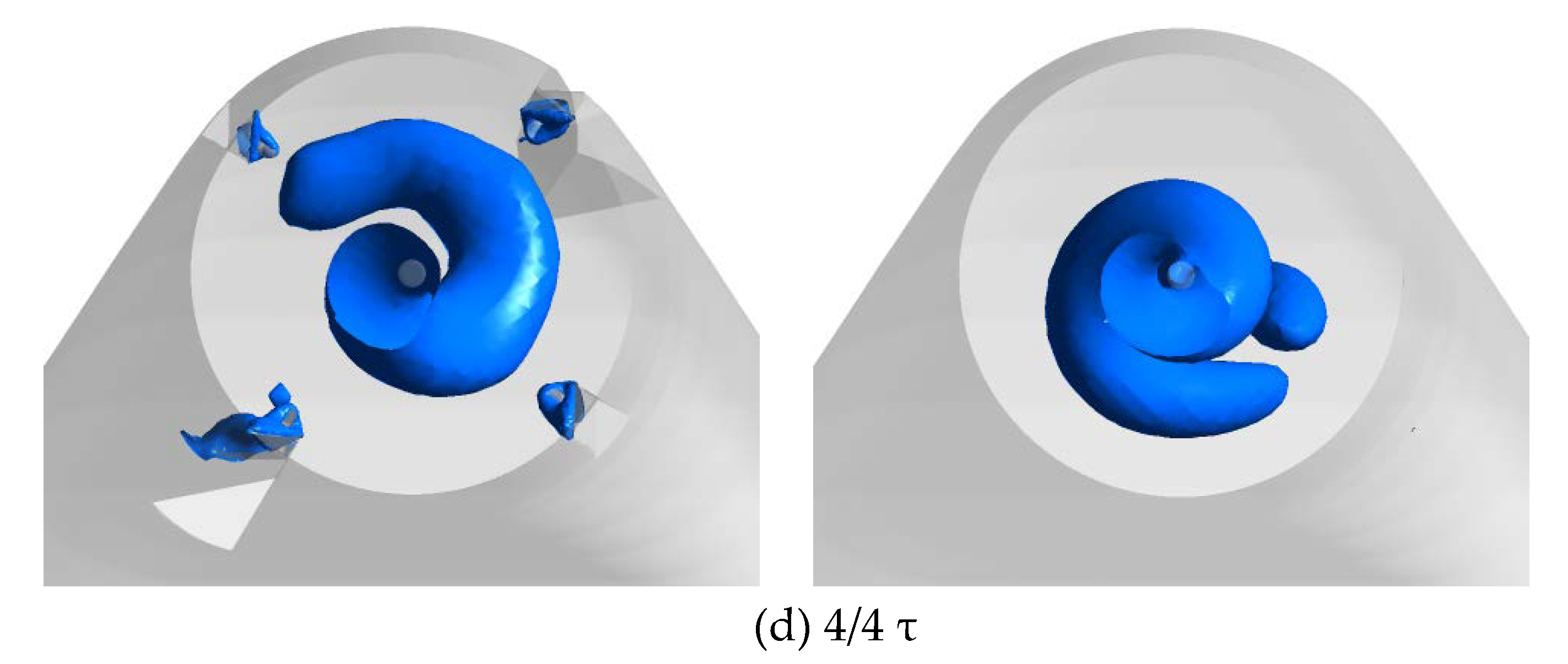
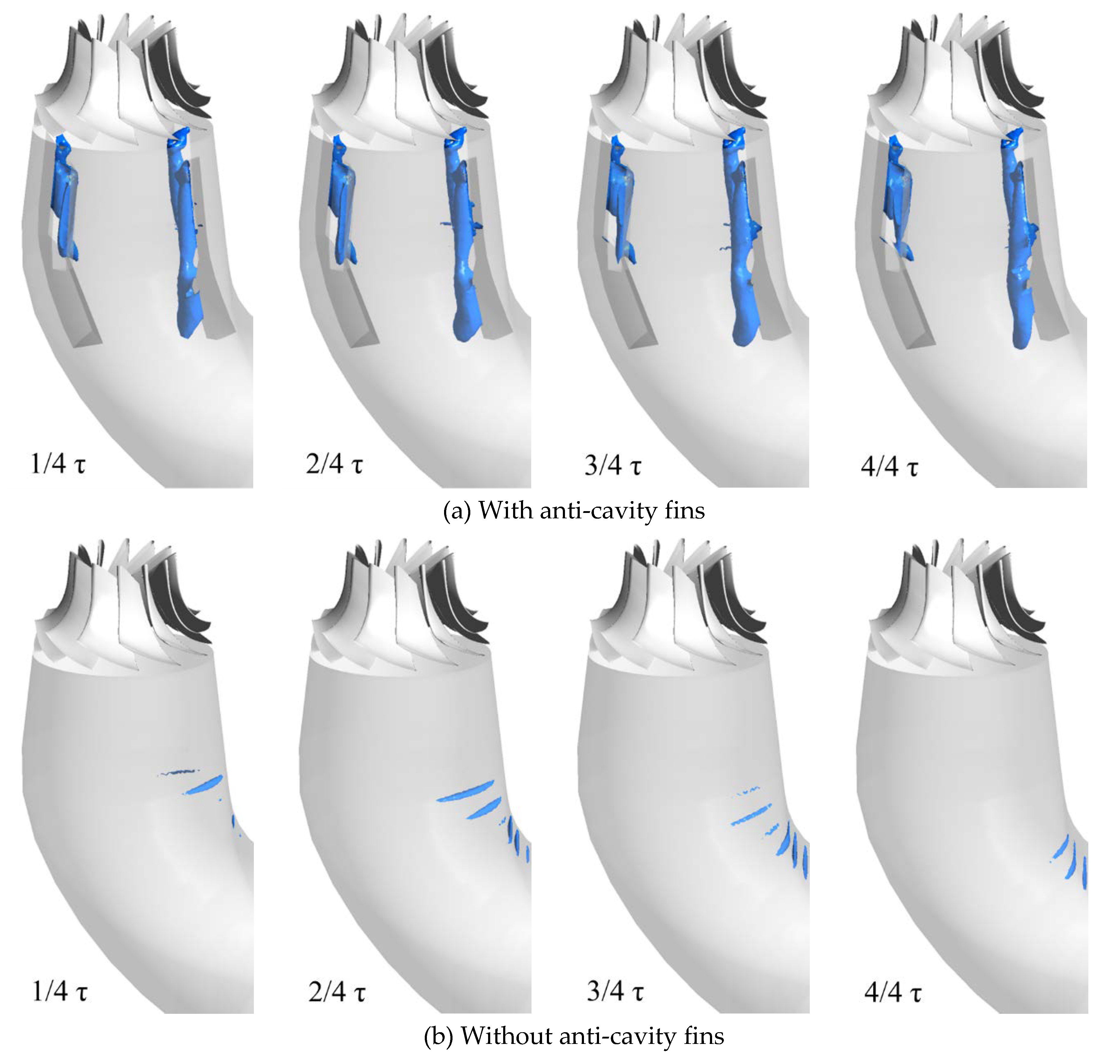
The above analyses reveal that at the observed GV of 16°, the head loss difference in the DT was the greatest, and the effects of the anti-cavity fins were significantly observed. Figure 13 presents a more detailed analysis of the internal flow characteristics of the same GV; it investigates the influence of the anti-cavity fins by comparing the iso-surface distribution of the pressure in the DT during the last revolution of the runner with the top view of the runner. The pressure value was determined to be the same as that used in Figure 8. Depending on time and irrespective of the inclusion of anti-cavity fins, the vortex ropes were maintained at similar maximum rotating diameters. Therefore, the effects of the anti-cavity fins decreased the maximum vertical length of the vortex rope, whereas the maximum rotating diameters were not significantly affected by the inclusion of anti-cavity fins.

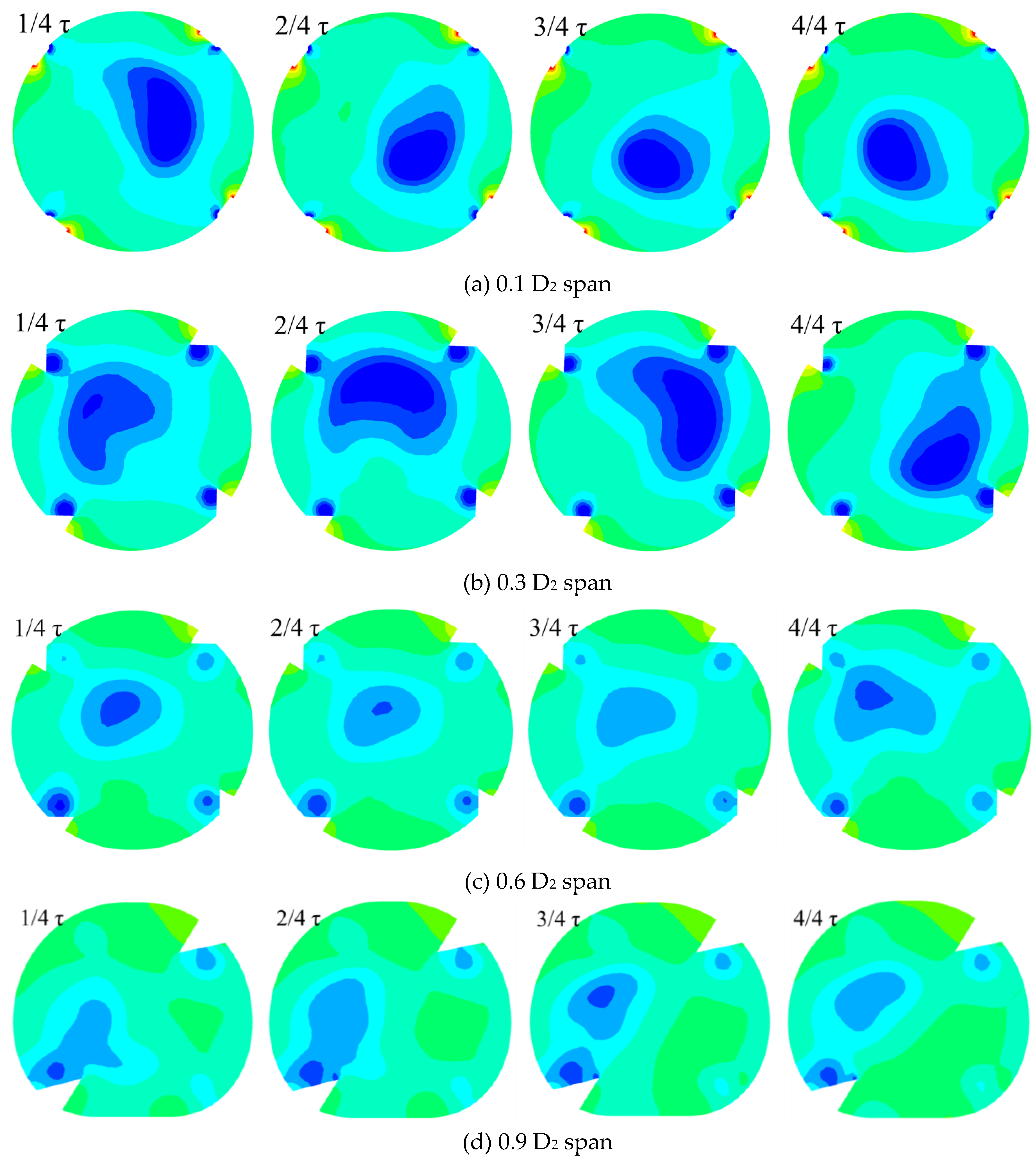
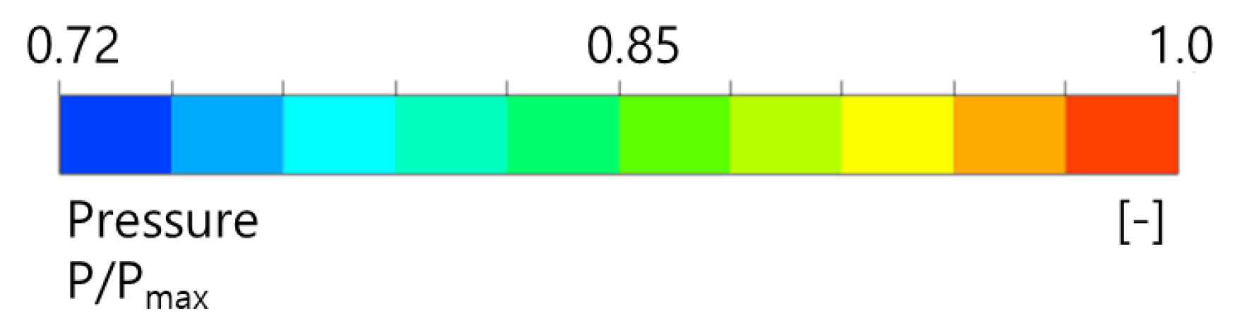
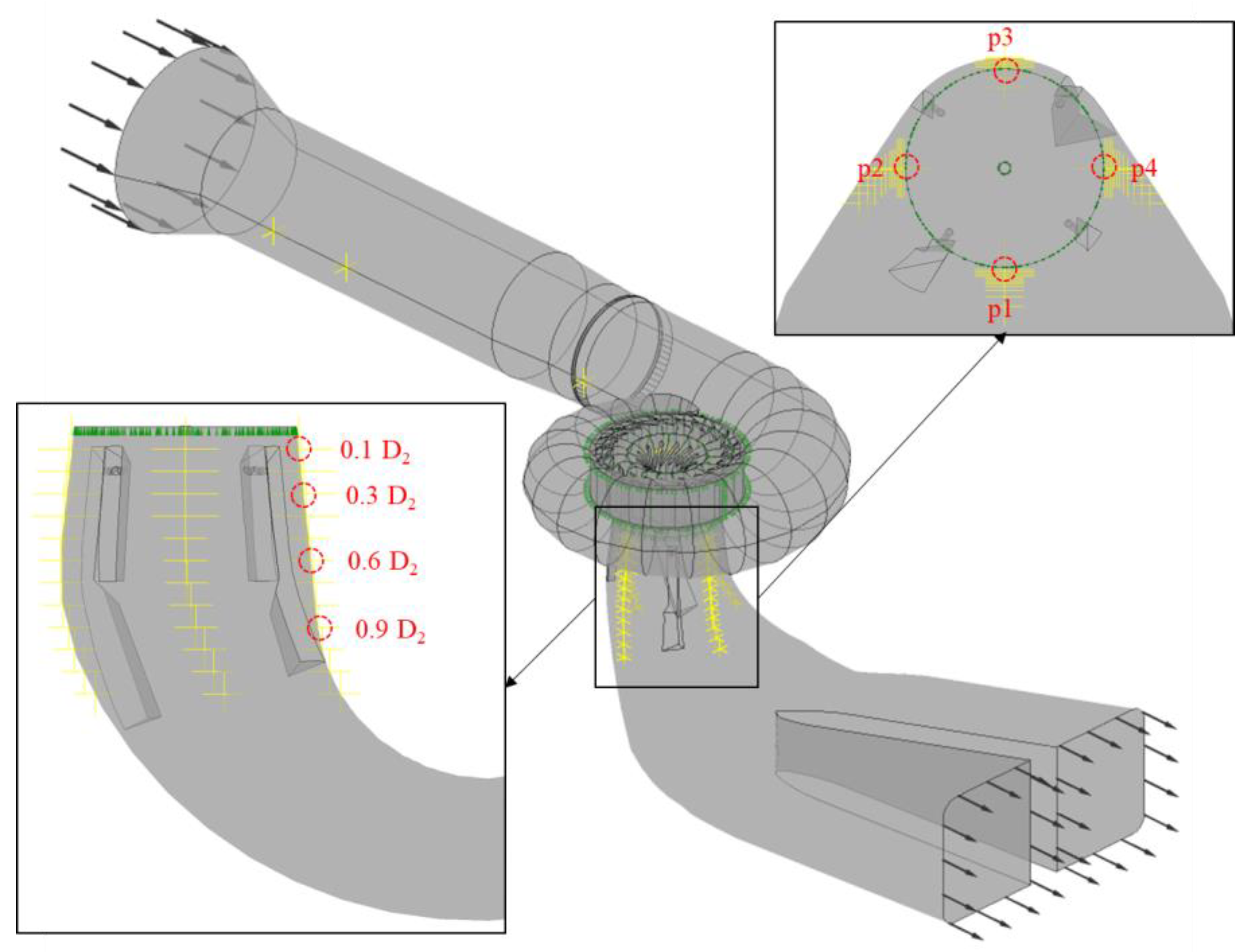
To investigate the effect of the anti-cavity fins in detail, Figure 14 and Figure 15 present the pressure distributions on the observed cross-sections (as shown in Figure 1) at the GV at 16° with and without anti-cavity fins, respectively. The cross-sections were examined at 0.1, 0.3, 0.6, and 0.9 D₂ in the direction of flow from the inlet of the DT, and the pressure values were normalized by the value of maximum pressure. The low-pressure regions in each cross-section of the pressure distributions were maintained with similar diameters, depending on time, and there was a tendency for the low-pressure regions to gradually decrease along the direction of flow. Furthermore, Figure 14 indicates that the low-pressure regions were clearly developed up to the cross-section of 0.3 D₂; however, because of the influence of the anti-cavity fins, these regions decreased considerably from 0.6 D₂. Meanwhile, the low-pressure regions were formed near the anti-cavity fins. It can be regarded that these regions were induced by the resistance of the anti-cavity fins to the tangential component of the absolute velocity, which increased as flow rate decreased as shown in Figure 10 (velocity triangle). Thus, via the low-pressure regions generated near the anti-cavity fins in Figure 14b, the formation sites of the low-pressure regions in Figure 8 and Figure 13 can be confirmed. Figure 15 clearly shows the low-pressure regions in the DT up to the cross-section of 0.9 D₂ without anti-cavity fins. Actually, the existing DT plays a role of recovering the static pressure in the flow; however in the low flow rate condition, the low-pressure regions indicated by the vortex rope with precession decreased with the anti-cavity fins rather than the decrease through the role of the DT itself. Therefore, it can be concluded that the anti-cavity fins effectively suppressed the generation of the vortex rope in the DT, particularly by decreasing the vertical length rather than by modifying the rotating diameters.

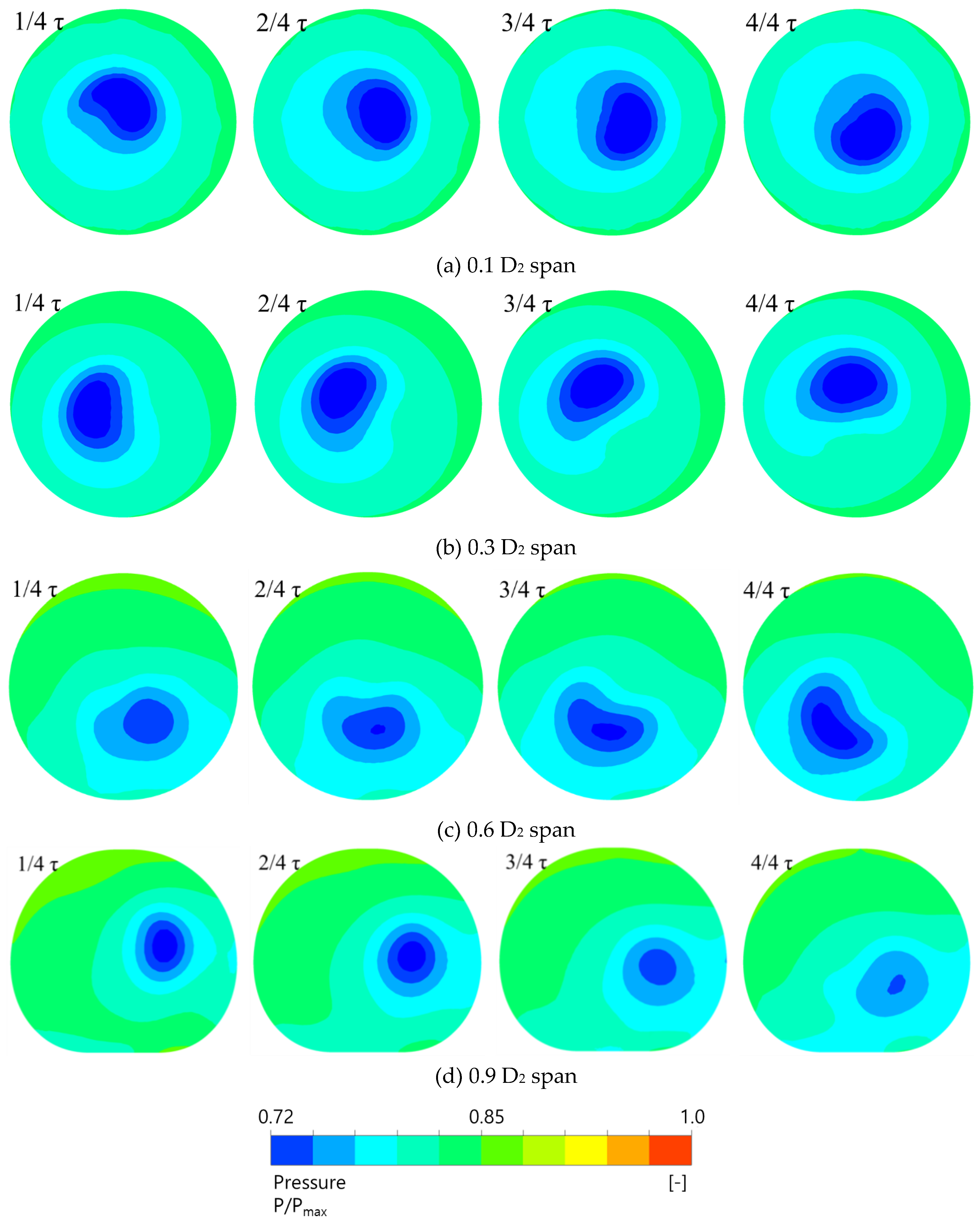
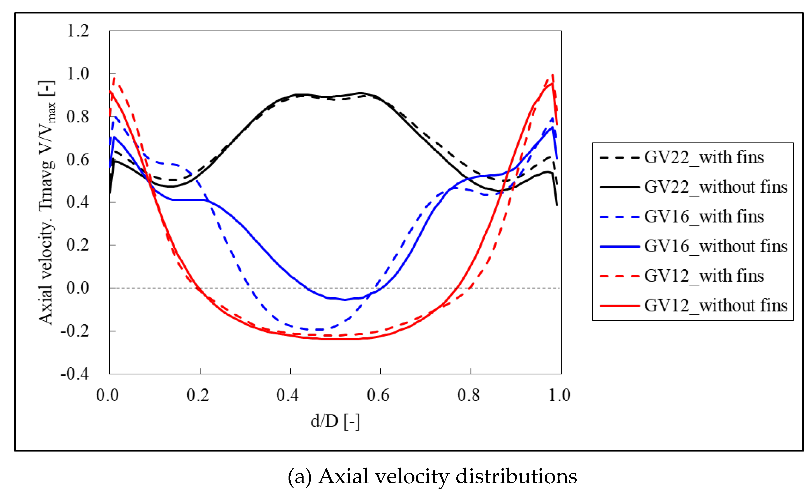
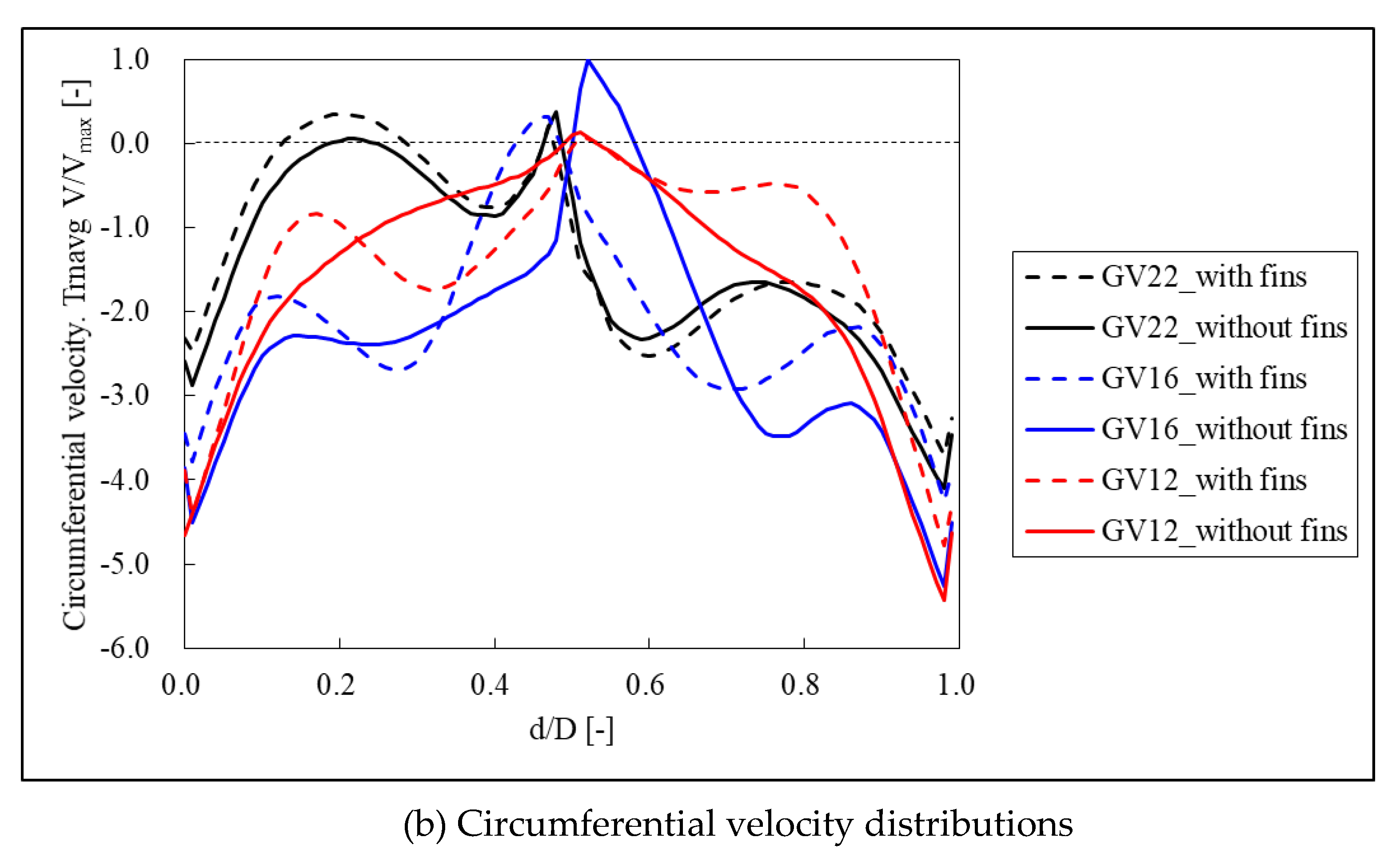
To analyze the influence of the anti-cavity fins at GVs at 22°, 16°, and 12°, the time-averaged axial and circumferential velocity components were compared on the observed line of 0.6 D₂ (in Figure 1) in the DT, as shown in Figure 16. The abscissa indicates the measurement location relative to the diameter from the wall (0) to the wall (1) of the DT, and the velocity values were normalized by the value of maximum velocity. Without the addition of anti-cavity fins, the axial velocity of the GV at 22°, as shown in Figure 16a, decreased slightly near to the wall, whereas the relatively small velocity range altered according to the anti-cavity fins.

However, the overall greatest difference in the axial velocity distribution was shown by the GV at 16° relative to the anti-cavity fins, and the backflow occurred near d/D = 0.5. With the GV at 12°, the backflow was generated in a relatively wide range of d/D = 0.2–0.8. A complicated internal flow without a vortex rope was demonstrated, and the difference in axial velocity was not shown to vary significantly according to the use of anti-cavity fins. Therefore, the anti-cavity fins had a relatively significant effect on the axial velocity at the GV at 16°; here, a vortex rope was formed, which was due to the shape characteristics of the anti-cavity fins installed in the axial direction concerning the flow direction.

In terms of circumferential velocity distributions, the anti-cavity fins near the wall of the DT revealed a slight difference at the GV at 22°, as presented in Figure 16b. The difference between the maximum and the minimum circumferential velocity was relatively greater at the GV at 16° without the anti-cavity fins; the addition of anti-cavity fins effectively reduced this difference. Furthermore, because of the complicated internal flow, a difference in the circumferential velocity distribution was exhibited along with the anti-cavity fins at the GV at 12°. Therefore, this study considers that the anti-cavity fins influenced the velocity component in the circumferential direction rather than the axial direction in the DT; the internal flow was mainly influenced under the low flow rate conditions, during which the vortex rope was generated.

4.3. Unsteady Pressure Characteristics Relative to the Anti-Cavity Fins in the Draft Tube

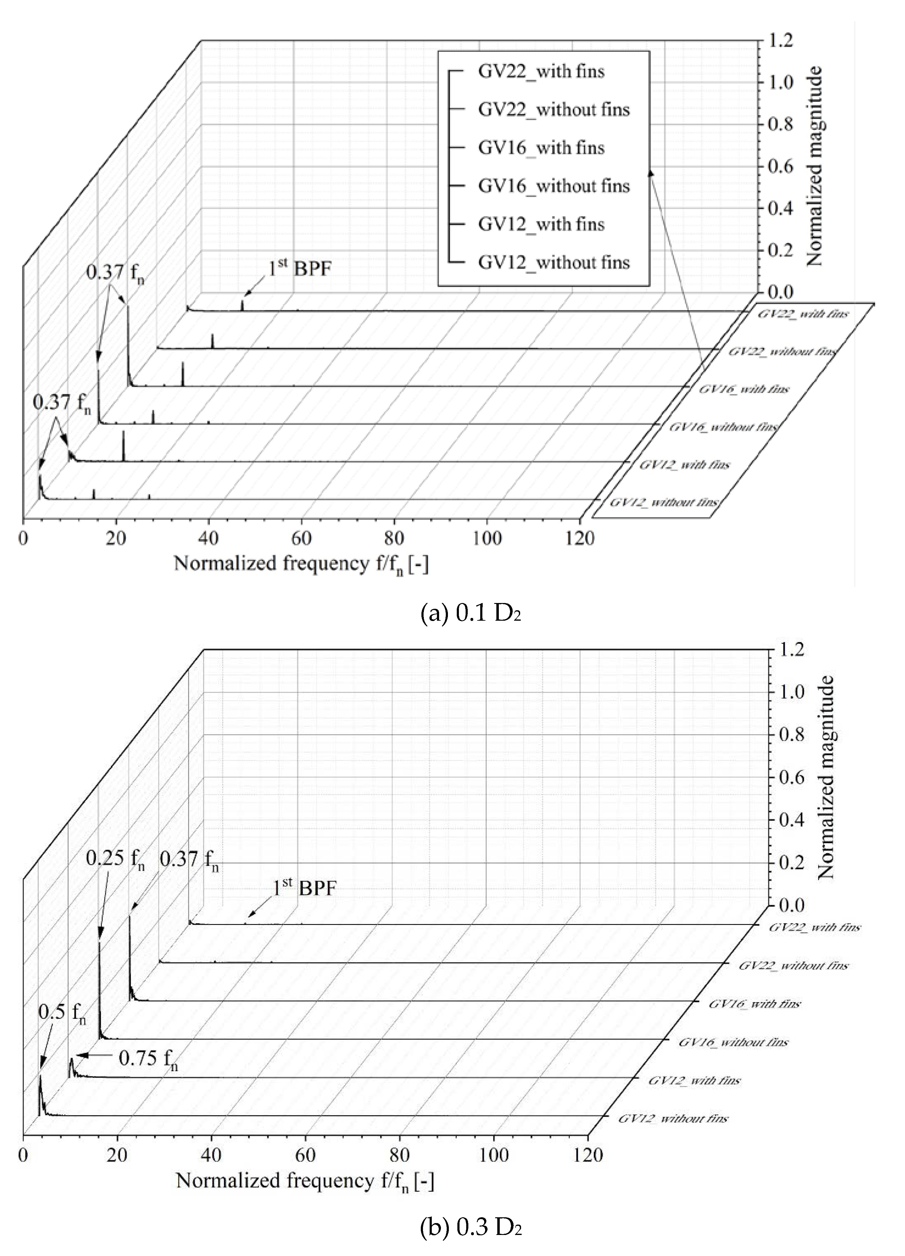
To investigate the unsteady pressure characteristics according to the use of anti-cavity fins in the DT, this study compared the unsteady pressures obtained via fast Fourier transformation (FFT) analysis with GVs at 22°, 16°, and 12°, as shown in Figure 17. The pressure measuring points of 0.1, 0.3, 0.6, and 0.9 D₂ were used in the flow direction on the DT wall, and the value for the highest pressure was used for each height from the four measuring points (p1–p4), as indicated in Figure 4. The maximum magnitude normalized the pressure values, and the frequency was normalized by the rotational frequency, f_n, of the Francis turbine model. The highest first blade passing frequency (BPF) was shown on the 0.1 D₂ at the GV at 22° as the BEP condition. However, at the normalized frequency of 0.37 f_n in the low-frequency region, relatively high-pressure characteristics were demonstrated before the first BPF at the GV at 16°, as the vortex rope with precession developed compared with other GV conditions. Previously, Kim et al. [25] numerically investigated similar unsteady pressure phenomena in the low-frequency region due to the vortex rope in the DT. Furthermore, the addition of anti-cavity fins at a measuring height of 0.1 D₂ slightly increased the unsteady pressure at the GV at 16°. This was due to the effect of the anti-cavity fins in reducing the length of the vortex rope of the GV at 16°, as can be seen in Figure 8, Figure 14 and Figure 15. However, the vortex rope remained near the inlet of the DT.

Unsteady pressure characteristics were exhibited at the normalized frequency of 0.37 f_n and near the low-frequency regions before the first BPF at the GV at 12°, where a complicated internal flow without a vortex rope was evident. At all the observed GVs, the first BPF was gradually decreased from 0.3 D₂ (shown in Figure 17b) in the flow direction. Without the addition of anti-cavity fins, the GV at 16° at 0.3 D₂ demonstrated greater unsteady pressure characteristics at the normalized frequency of 0.25 f_n than it did with them. 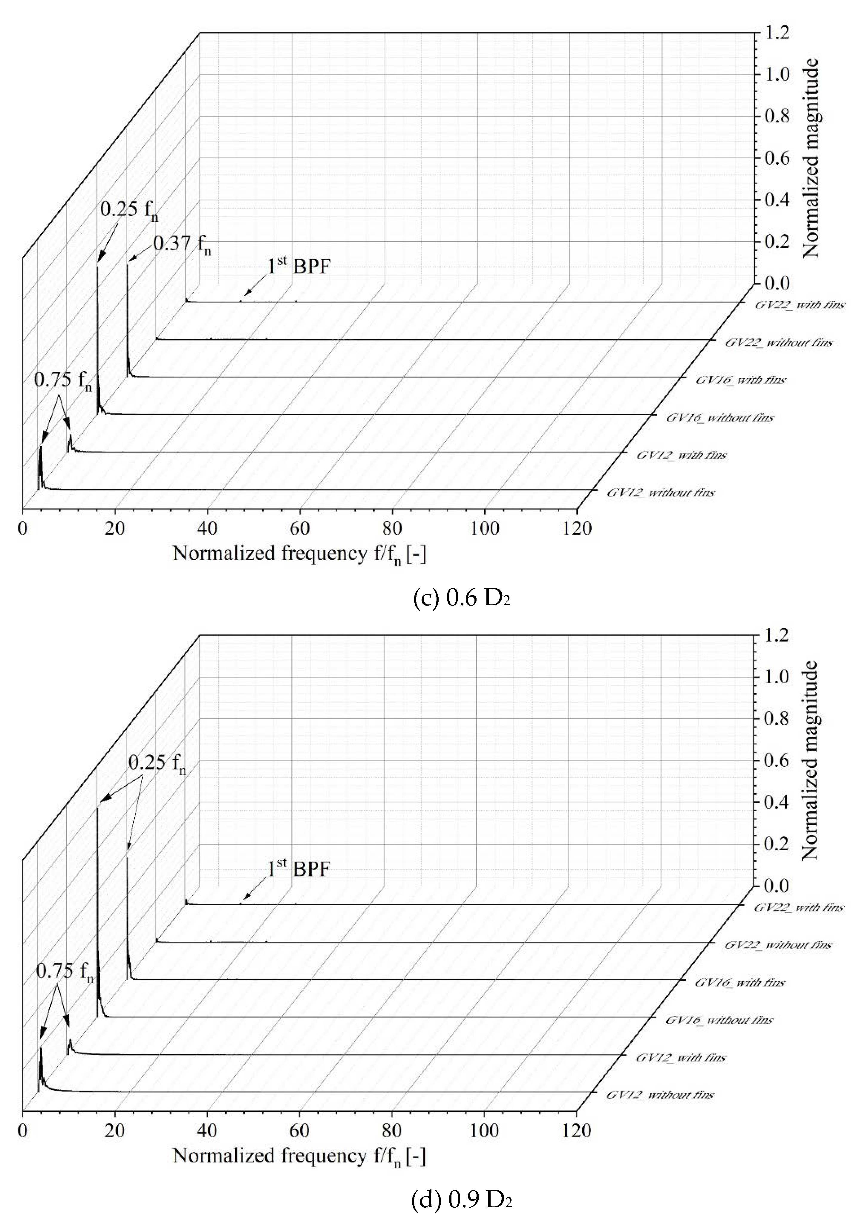Unsteady pressure at the 12° GV at 0.3 D₂ increased in the normalized frequency range of 0.5–0.75 f_n, which was greater than the magnitude at 0.1 D₂. In Figure 17c, both unsteady pressures at the GV at 16° increased more at the normalized frequency of 0.25–0.37 f_n compared with those at 0.3 D₂; at the 12° GV, the normalized frequency of 0.75 f_n was shown to be similar to the magnitude of 0.3 D₂. As is evident in Figure 17d, the GV at 12° exhibited similar unsteady pressure characteristics to those at 0.6 D₂.

The differences in the maximum magnitude of unsteady pressure due to anti-cavity fins were noticeable in the GV at 16°, and the magnitude of unsteady pressure with the anti-cavity fins was similar to the magnitude with anti-cavity fins at 0.6 D₂. Therefore, the unsteady pressure characteristics increased along the flow direction in the DT under conditions of low flow rate with a developed vortex rope; the use of anti-cavity fins effectively decreased the unsteady pressures. Particularly, the application of anti-cavity fins resulted in an approximate 41% reduction in the maximum magnitude of unsteady pressure at the 16° GV at a measured height of 0.9 D₂.

5. Conclusions

This study performed unsteady-state RANS analyses to investigate the effects of anti-cavity fins in the DT of a Francis turbine model on unsteady internal flow and pressure characteristics under low flow rate conditions. Reductions of around 0.5%–1.0% in hydraulic performance within the range of observed GV angles were observed, and the head losses of each component in the Francis turbine model were compared via the application of anti-cavity fins. Furthermore, the magnitudes and locations of the vortex ropes in the DT were verified via iso-surface distributions both with and without anti-cavity fins according to varying flow rate conditions. The existence of low-pressure regions due to flow resistance at the prominent air injection outlet on the anti-cavity fins was also confirmed.

The causes of the complicated flow phenomena in the DT respective to varying flow rates were confirmed via an analysis of the velocity triangles at the runner outlet. Furthermore, quantitative and qualitative investigations were conducted using the flow angle distributions at the runner outlet and the streamline distributions in the DT. A comparison of velocity distributions on the observed line confirmed the effects of the anti-cavity fins on the axial and circumferential velocity components in the DT. Furthermore, FFT analyses confirmed that the largest magnitudes of unsteady pressure were observed under low flow rate conditions with developed vortex ropes. There was a tendency for these magnitudes to gradually increase along the flow direction in the DT. Additionally, an approximate 41% reduction in the maximum unsteady pressure was confirmed with the application of anti-cavity fins.

Therefore, the use of anti-cavity fins was confirmed to affect the degradation of hydraulic performance under conditions of low flow rate, including BEP; however, the effects of reducing the unsteady pressure in the low-frequency regions were confirmed in the DT, which induced operational instability in the Francis turbine model. Thus, the anti-cavity fins can be presented as one alternative to suppress unsteady pressure fluctuations with vortex rope in the DT. Furthermore, by minimizing the loss induced by the anti-cavity fins through the optimization of the shape and length of the anti-cavity fins, it can be expected to improve the hydraulic performance with suppressing pressure fluctuation effectively. In the addition, based on the results of this research, the unsteady flow and pressure phenomena in the DT will be investigated in a future study by injecting air into the DT.

References

1. Kim, S.J.; Choi, Y.S.; Cho, Y.; Choi, J.W.; Kim, J.H. Effect of Runner Blade Thickness on Flow Characteristics of a Francis Turbine Model at Low Flowrates. J. Fluids Eng. 2020, 142, 031104. [Google Scholar] [CrossRef]
2. Nishi, M.; Liu, S. An outlook on the draft-tube-surge study. Int. J. Fluid Mach. Syst. 2013, 6, 33–48. [Google Scholar] [CrossRef] [Green Version]
3. Eichhorn, M.; Taruffi, A.; Bauer, C. Expected load spectra of prototype Francis turbines in low-load operation using numerical simulations and site measurements. J. Phys. Conf. Ser. 2017, 813, 012052. [Google Scholar] [CrossRef] [Green Version]
4. Feng, J.J.; Li, W.F.; Wu, H.; Lu, J.L.; Liao, W.L.; Luo, X.Q. Investigation on pressure fluctuation in a Francis turbine with improvement measures. IOP Conf. Ser. Earth Environ. Sci. 2014, 22, 032006. [Google Scholar] [CrossRef] [Green Version]
5. Favrel, A.; Müller, A.; Landry, C.; Yamamoto, K.; Avellan, F. Study of the vortex-induced pressure excitation source in a Francis turbine draft tube by particle image velocimetry. Exp. Fluids 2015, 56, 215. [Google Scholar] [CrossRef]
6. Susan-Resiga, R.; Muntean, S.; Stein, P.; Avellan, F. Axisymmetric swirling flow simulation of the draft tube vortex in Francis turbines at partial discharge. Int. J. Fluid Mach. Syst. 2009, 2, 295–302. [Google Scholar] [CrossRef]
7. Nicolet, C.; Zobeiri, A.; Maruzewski, P.; Avellan, F. Experimental investigations on upper part load vortex rope pressure fluctuations in Francis turbine draft tube. Int. J. Fluid Mach. Syst. 2011, 4, 179–190. [Google Scholar] [CrossRef] [Green Version]
8. Zuo, Z.; Liu, S.; Liu, D.; Qin, D. Numerical predictions and stability analysis of cavitating draft tube vortices at high head in a model Francis turbine. Sci. China Technol. Sci. 2014, 57, 2106–2114. [Google Scholar] [CrossRef]
9. Altimemy, M.; Attiya, B.; Daskiran, C.; Liu, I.H.; Oztekin, A. Mitigation of flow-induced pressure fluctuations in a Francis turbine operating at the design and partial load regimes—LES simulations. Int. J. Heat Fluid Flow 2019, 79, 108444. [Google Scholar] [CrossRef]
10. Susan-Resiga, R.; Vu, T.C.; Muntean, S.; Ciocan, G.D.; Nennemann, B. Jet control of the draft tube vortex rope in Francis turbines at partial discharge. In Proceedings of the 23rd IAHR Symposium Conference, Yokohama, Japan, 17–21 October 2006; pp. 67–80. [Google Scholar]
11. Li, W.F.; Feng, J.J.; Wu, H.; Lu, J.L.; Liao, W.L. Numerical investigation of pressure fluctuation reducing in draft tube of Francis turbines. Int. J. Fluid Mach. Syst. 2015, 8, 202–208. [Google Scholar] [CrossRef] [Green Version]
12. Anup, K.C.; Lee, Y.H.; Thapa, B. CFD study on prediction of vortex shedding in draft tube of Francis turbine and vortex control techniques. Renew. Energy 2016, 86, 1406–1421. [Google Scholar]
13. Chen, Z.; Choi, Y.D. Suppression of cavitation in the draft tube of Francis turbine model by J-Groove. Proc. Inst. Mech. Eng. Part C J. Mech. Eng. Sci. 2019, 233, 3100–3110. [Google Scholar] [CrossRef]
14. International Electrotechnical Commission. Hydraulic Turbines, Storage Pumps and Pump-Turbines—Model Acceptance Tests, Standard No. IEC 60193; International Electrotechnical Commission: Geneva, Switzerland, 1999. [Google Scholar]
15. ANSYS CFX-19.1, ANSYS CFX-Solver Theory Guide; ANSYS Inc.: Canonsburg, PA, USA, 2018.
16. Richardson, L.F., IX. The approximate arithmetical solution by finite differences of physical problems involving differential equations, with an application to the stresses in a masonry dam. Philos. Trans. R. Soc. Lond. Ser. A Contain. Pap. Math. Phys. Character 1911, 210, 307–357. [Google Scholar]
17. Richardson, L.F.; Gaunt, J.A., VIII. The deferred approach to the limit. Philos. Trans. R. Soc. Lond. Ser. A Contain. Pap. Math. Phys. Character 1927, 226, 299–361. [Google Scholar]
18. Celik, I.B.; Ghia, U.; Roache, P.J.; Freitas, C.J.; Coleman, H.; Raad, P.E.; Celik, I.; Freitas, C.; Coleman, H.P. Procedure for estimation and reporting of uncertainty due to discretization in CFD applications. J. Fluids Eng. 2008, 130, 078001. [Google Scholar]
19. Kim, S.J.; Choi, Y.S.; Cho, Y.; Choi, J.W.; Hyun, J.J.; Joo, W.G.; Kim, J.H. Analysis of the Numerical Grids of a Francis Turbine Model through Grid Convergence Index Method. KSFM J. Fluid Mach. 2020, 23, 16–22. (In Korean) [Google Scholar] [CrossRef]
20. Zwart, P.J.; Gerber, A.G.; Belamri, T. A two-phase flow model for predicting cavitation dynamics. In Proceedings of the Fifth International Conference on Multiphase Flow, Yokohama, Japan, 30 May–4 June 2004. [Google Scholar]
21. Egorov, Y.; Menter, F. Development and application of SST-SAS turbulence model in the DESIDER project. Adv. Hybrid RANS-LES Model 2008, 261–270. [Google Scholar] [CrossRef]
22. Menter, F.R.; Egorov, Y. The scale-adaptive simulation method for unsteady turbulent flow predictions. Part 1: Theory and model description. Flow Turbul. Combust. 2010, 85, 113–138. [Google Scholar] [CrossRef]
23. Korea Agency for Infrastructure Technology Advancement, Report Development of Construction Technology for Medium Sized Hydropower Plant; Report No. 17IFIP-B128593-01; Anyang-si, Korea, 2017; Available online: http://icities4greengrowth.in/people/agency/kaia-korea-agency-infrastructure-technology-advancement (accessed on 20 May 2020).
24. Chen, Z.; Singh, P.M.; Choi, Y.D. Francis turbine blade design on the basis of port area and loss analysis. Energies 2016, 9, 164. [Google Scholar] [CrossRef] [Green Version]
25. Kim, S.J.; Suh, J.W.; Choi, Y.S.; Park, J.; Park, N.H.; Kim, J.H. Inter-Blade Vortex and Vortex Rope Characteristics of a Pump-Turbine in Turbine Mode under Low Flow Rate Conditions. Water 2019, 11, 2554. [Google Scholar] [CrossRef] [Green Version]
Figure 1. (a) 3-D model of the DT with (b) location of anti-cavity fins in the Francis turbine model.
Energies 13 02806 g001aEnergies 13 02806 g001b
Figure 2. Numerical grids used in the Francis turbine model.
Energies 13 02806 g002
Figure 3. Comparisons of efficiency and flow rate with observed numerical grids in the Francis turbine model.
Energies 13 02806 g003
Figure 4. Pressure measurement points in the Francis turbine model.
Energies 13 02806 g004
Figure 5. Comparison of the conversed numerical results and the experimental results of a full-scale Francis turbine.
Energies 13 02806 g005
Figure 6. Head loss distribution in the main components of the Francis turbine model.
Energies 13 02806 g006
Figure 7. Iso-surface distributions of pressure in the DT during one runner revolution at a GV of 22°: (a) with anti-cavity fins; and (b) without anti-cavity fins.
Energies 13 02806 g007
Figure 8. Iso-surface distributions of pressure in the DT during one runner revolution at a GV of 16°: (a) with anti-cavity fins; and (b) without anti-cavity fins.
Energies 13 02806 g008aEnergies 13 02806 g008b
Figure 9. Iso-surface distributions of pressure in the DT during one runner revolution at a GV of 12°: (a) with anti-cavity fins; and (b) without anti-cavity fins.
Energies 13 02806 g009
Figure 10. Velocity triangle on the mid-span at GVs of 22°, 16°, and 12°.
Energies 13 02806 g010
Figure 11. Streamline distributions in the DT (left column) with and (right column) without anti-cavity fins at GVs of (a) 22°, (b) 16°, and (c) 12°.
Energies 13 02806 g011
Figure 12. (a) Absolute and (b) relative flow angle distributions along the spanwise direction at the outlet of the runner at GVs of 22°, 16°, and 12°.
Energies 13 02806 g012
Figure 13. Iso-surface distributions of pressure in the DT by the top view from the runner at the GV at 16° (left column) with and (right column) without anti-cavity fins during one revolution of the runner. (a) 1/4, (b) 2/4, (c) 3/4, and (d) 4/4 τ.
Energies 13 02806 g013aEnergies 13 02806 g013b
Figure 14. Pressure distributions on observed spans in the DT with anti-cavity fins at the GV at 16° during one revolution of the runner: span locations at (a) 0.1, (b) 0.3, (c) 0.6, and (d) 0.9 D2.
Energies 13 02806 g014aEnergies 13 02806 g014b
Figure 15. Pressure distributions on observed spans in the DT without anti-cavity fins at the GV at 16° during one revolution of the runner: span locations at (a) 0.1, (b) 0.3, (c) 0.6, and (d) 0.9 D2.
Energies 13 02806 g015
Figure 16. (a) Axial and (b) circumferential velocity distributions on the observed line in the DT.
Energies 13 02806 g016aEnergies 13 02806 g016b
Figure 17. Normalized unsteady pressure characteristics along the flow direction in the DT: (a) 0.1, (b) 0.3, (c) 0.6, and (d) 0.9 D2.
Energies 13 02806 g017aEnergies 13 02806 g017b