Article

Improvements on a Sensorless Scheme for a Surface-Mounted Permanent Magnet Synchronous Motor Using Very Low Voltage Injection

by
Jaime Pando-Acedo
*,
Enrique Romero-Cadaval
,
Maria Isabel Milanes-Montero
and
Fermin Barrero-Gonzalez
Department of Electrical, Electronic and Automation Engineering, University of Extremadura, 06006 Badajoz, Spain
*
Author to whom correspondence should be addressed.
Energies 2020, 13(11), 2732; https://doi.org/10.3390/en13112732
Submission received: 21 April 2020 / Revised: 18 May 2020 / Accepted: 26 May 2020 / Published: 29 May 2020
(This article belongs to the Special Issue Modeling, Simulation and Control of Electric Drive Systems)

Abstract

:
Sensorless control of electrical drives is still a difficult task, especially in the lower speed region. Moreover, when the machine has a low saliency such as in the case of Surface Mounted Permanent Magnet Synchronous Motor (SMPMSM), high frequency injection techniques are even more challenging. In this paper, an enhanced demodulation algorithm for the sensorless control of a SMPMSM is proposed. The new scheme uses the high frequency injection in the Synchronous Reference Frame (SRF) and employs also the negative sequence content of the measured current for improved accuracy. This allows an improved performance with a lower amplitude of the injected signal, thus reducing the noise and additional losses in the motor. It is found that, by using both components with the algorithm developed the estimation ripple can be greatly reduced and the system can operate properly with a voltage injection of only 2.17% of the rated motor voltage, which is lower than most found in the literature, specially for low saliency machines. Simulations tests are carried out for the validation of the proposed method and experimental results in a 6.7 kW SMPMSM confirm its usefulness and correct operation with a reduced voltage injection, both in no-load and load conditions, for different low speeds, including start-up.

Graphical Abstract

1. Introduction

The Permanent Magnet Synchronous Machine (PMSM) is widely regarded as one of the most used AC machines, along with the Induction Machine. In particular, it has found its place in the Electric Vehicle field. The main reasons include high efficiency, high torque to size ratio and excellent robustness and reliability. Although there are several control strategies, the main one found in the literature and industry for these machines is the Field-Oriented Control (FOC), which continues to be target of research and development [1,2,3]. The key issue of the FOC implementation is the correct acquisition of the rotor position, usually by means of an optical or magnetic transducer (encoder), or extra windings in the rotor (resolver). This introduces extra complexity in the system as well as increases the manufacturing cost and reduces the reliability. Moreover, the use of optical encoders also represents the source of measuring errors which could deteriorate the control performance [4]. Tackling these issues motivates the research on the sensorless control strategies, which has been a prolific research line for the last decades [5,6,7]. Getting rid of the extra hardware would represent a great benefit for many industrial and commercial applications.
Depending on the speed range, sensorless strategies can be roughly classified into two big groups: model-based and high-frequency signal injection. The former is usually employed in the higher speed regions and has the advantage of being relatively easy to implement and having good accuracy [8,9,10]. However, due to their dependency on the back-electromotive force, they exhibit poor results in the lower speed regions. The latter makes use of the machine anisotropy to recover the rotor’s position information by injecting a high frequency signal along with the fundamental excitation [11,12,13,14]. Although they have proven to provide good results, the high frequency signal produces noise, vibrations and extra losses. They can also interfere with the controllers, rendering the system unstable in the worst case scenario.
Focusing on the signal injection algorithms, the classification can be divided into several groups. The injection can be done in the stationary reference frame [15] or in the synchronous reference frame (SRF) [13,16]. The first one uses a rotating voltage vector injection, which can cause ripple in the i q current and therefore, vibrations. To overcome this problem, the second one injects a pulsating voltage in the estimated d axis. Both normally make use of filters for recovering the high frequency content, which deteriorates the bandwidth of the controllers [17]. However, pulsating injection have shown more precise estimations and its signal processing is simpler [18]. Nevertheless, some studies report convergence problems at the starting stage as well as steady state errors [18,19,20].
On recent research, the trend has been to use a square voltage signal for the estimation [14,18,21]. It has the advantage of being able to raise the injection frequency greatly. By doing so, the filters used in the processing of the signal can have higher cut-off frequencies or be omitted, achieving wider bandwidths. However, most of this demodulation techniques make use of the current derivatives, making them very sensitive to noise and inverter non linearities [21].
One of the greatest concerns in the literature is the magnitude of the voltage injection. In general, rising the injection frequency is desirable but it also means injecting higher voltages in order to have a good Signal to Noise ratio (S/N). Most of the research consulted need a signal in the range of 30–50 V [18,19,20,21,22,23], and only a few in the 10–30 V range [14,24]. Moreover, it can be observed in Table 1 that when the amplitude of the voltage injected is compared to the rated voltage of the machine tested, the ratios are still very high. This is also affected by the fact that in the case of Surface Mounted PMSM (SMPMSM), the spatial rotor saliency is quite low [25] and larger voltages are needed. Therefore, there is a need of further improving the demodulation methods in order to be able to extract as much information as possible [24,26].
This paper follows this trend and aims to lower the voltage needed for the sensorless control to work in a SMPMSM, making use of the pulsating injection in the estimated SRF. A new enhanced demodulation is proposed and experimentally validated to be able to develop a sensorless algorithm that is able to operate with a very low voltage injection.
The paper is structured as follows. First, the mathematical background for the problem is described, paying attention to the challenges it represents. Next, an enhanced demodulation algorithm is proposed and simulation tests are conducted for studying its usefulness. Finally, experimental procedures are carried out to validate the simulations, and conclusions from the work are drawn.

2. Problem Description

For the acquiring of the rotor position, a low amplitude carrier voltage will be injected into the machine, along with the fundamental excitation. This voltage is injected in the estimated rotor reference frame δ ^ and follows the expression
u c S = U c cos ( ω c t ) e j δ ^ ,
where U c is the amplitude of the voltage injected, ω c is the voltage angular frequency and δ ^ is the estimated position of the rotor, expressed in electrical radians. Figure 1 shows the phasor diagram for this kind of injection, also referred as pulsating. If the currents of the machine are separated into fundamental and carrier terms, the latter will be described by [11,13,26]
i c S = U c j 4 ω c l d l q [ ( l d + l q ) e j ( ω c t + δ ^ ) ( l d l q ) e j ( ω c t δ ^ + 2 δ ) ( l d + l q ) e j ( ω c t + δ ^ ) + ( l d + l q ) e j ( ω c t δ ^ + 2 δ ) ] ,
being l d , l q the direct and quadrature inductances of the machine and δ the real position of the rotor. Here we can appreciate four different terms, two rotating in the positive direction and the the other two rotating in the negative direction. Although there are other angles in the exponentials, since the injection frequency is selected to be much higher than the rotor’s one, the rotating direction of the vector is determined by the former.
As can be seen in (2), there are two terms containing the information of the rotor position δ . Any of these two can be used for the demodulation process. If this expression is taken to a reference frame rotating at an angular frequency of ω c t + δ ^ , the currents then will be
i c ( ω c t + δ ^ ) = i c S e j ( ω c t + δ ^ ) = U c j 4 ω c l d l q [ ( l d + l q ) ( l d l q ) e j ( 2 δ 2 δ ^ ) ( l d + l q ) e j 2 ω c t + ( l d l q ) e 2 δ 2 δ ^ 2 ω c t ] .
From (3), it can be seen that two terms have been displaced to higher frequencies around 2 ω c t . The error committed in the estimation can be expressed as
Δ δ = δ δ ^ .
If we keep the low frequency content in (3), assuming that the error is small enough so cos ( Δ δ ) = 1 and sin ( Δ δ ) = Δ δ , the expression becomes
i p ( ω c t + δ ^ ) = U c 2 ω c l d l q ( l d l q ) Δ δ + j l q .
In (5), it can be observed that the real part of the currents expressed in this reference frame is proportional to the error between the real rotor position and the one used for injecting the voltage u c S . This signal can be used by a controller for tracking the error and thus estimating the rotor position. A typical scheme for demodulating the signal using the expression above defined is shown in Figure 2. The carrier currents are separated from the fundamental excitation of the machine by means of a Band-Pass Filter (BPF). Afterwards, the real part is passed through a Low-Pass Filter (LPF) and fed to a Proportional-Integral (PI) controller for tracking.
At this point, some clarifications regarding the magnitude of the signal recovered should be made. Considering (5), the following can be concluded:
  • The amplitude of this signal is directly proportional to the error committed during the estimation, as well as the difference between the direct and quadrature inductances. This means that, for the case of a SMPMSM, this difference will be very small and so will be the signal recovered.
  • The signal is also directly proportional to the voltage injected but inversely proportional to the injection frequency. The amplitude of the voltage should be low and the frequency high enough, so there is no detriment in the main control algorithm of the system. However, for a good resolution of the recovered signal, the injection frequency should not be higher than f s / 6 , being f s the sampling frequency.
Taking into account those aspects, it is clear that the amplitude of the current used to track the error will be small. Another important issue will be the correct processing of this signal, to avoid distortion and maximize accuracy. Therefore, it is desirable to use all the possible information contained within the signal.

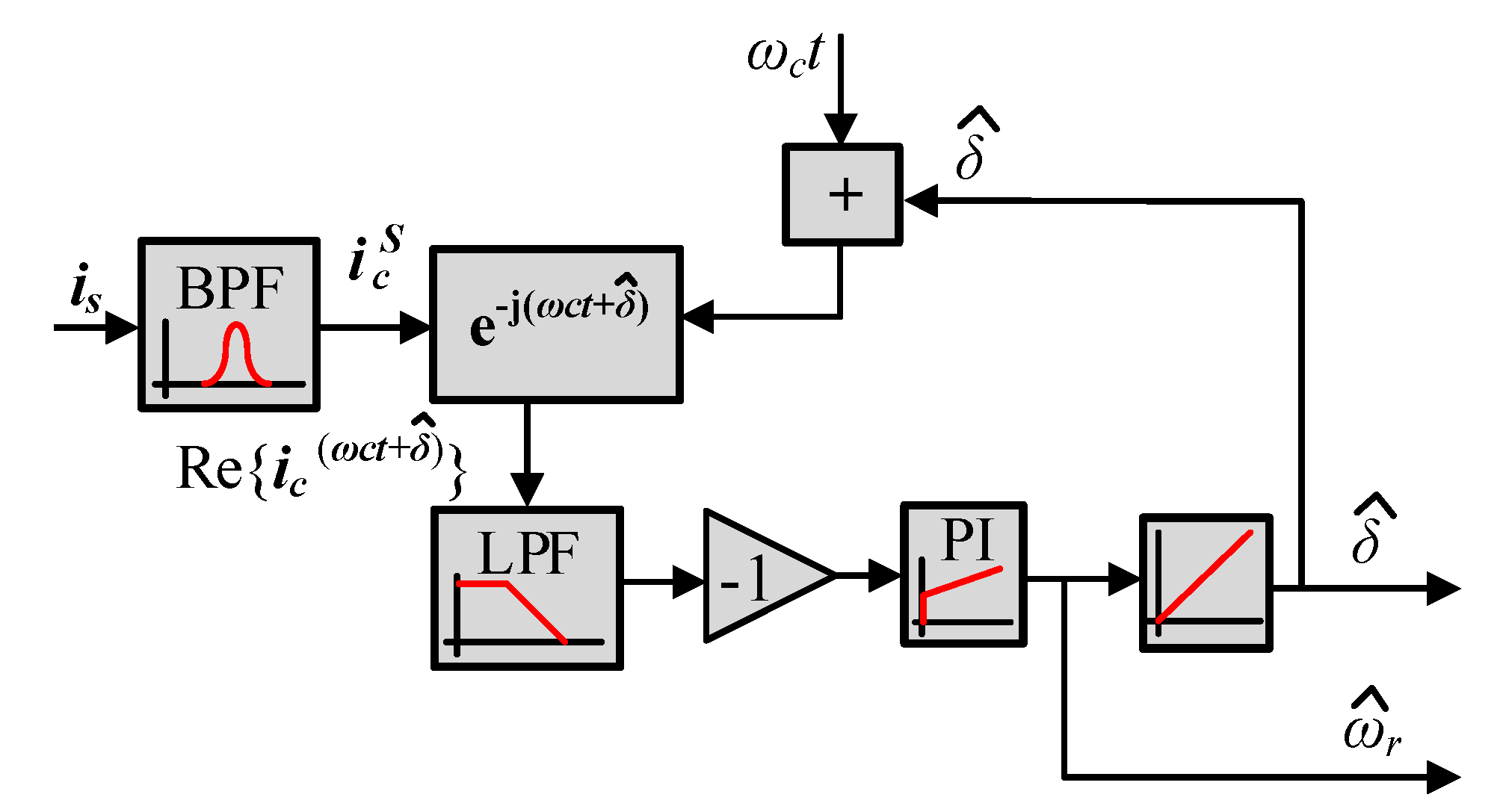
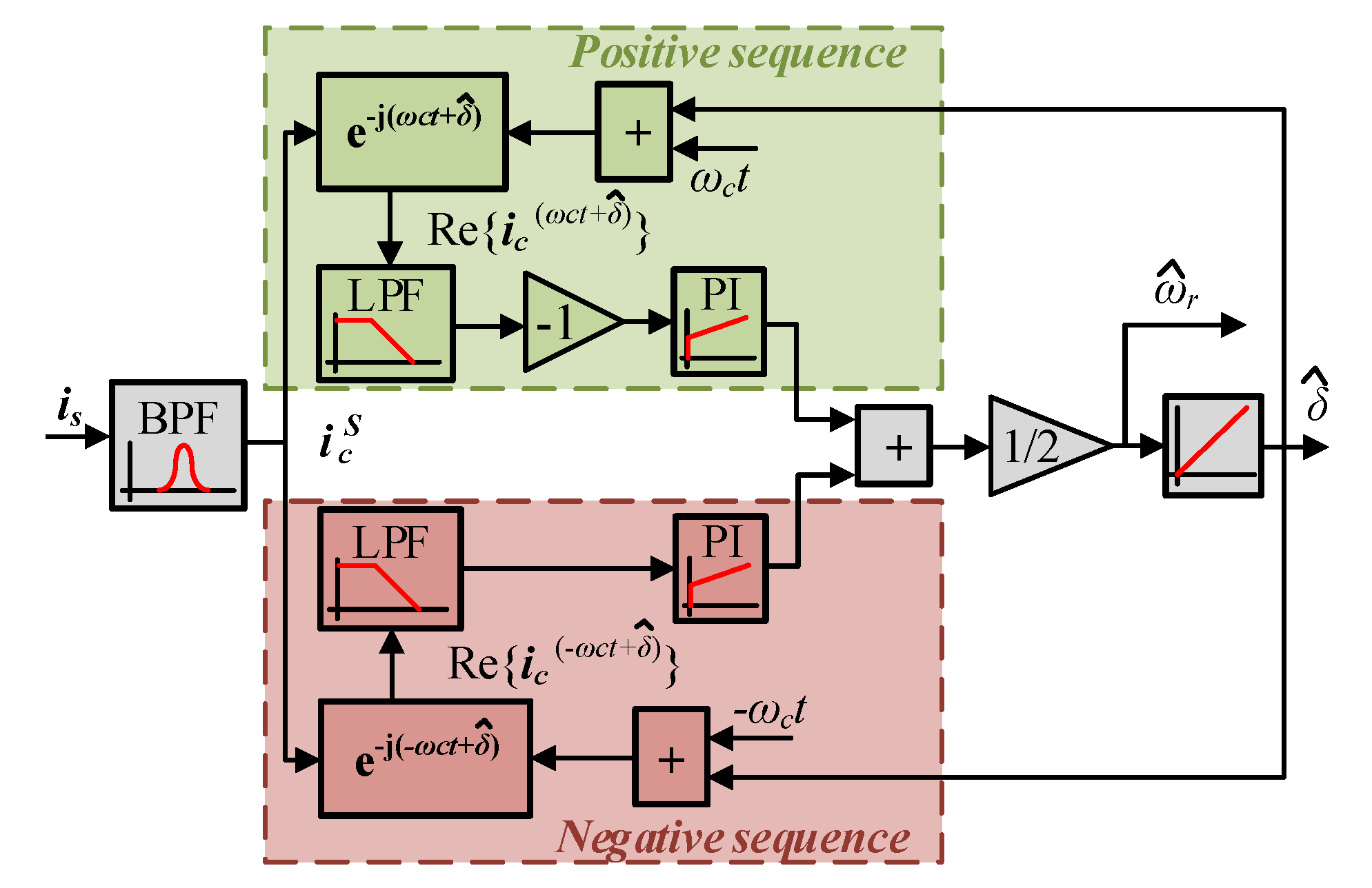
3. Enhanced Demodulation

As it was previously stated, there are two components of the carrier current i c S that contains the rotor information. In order to take advantage of the whole signal, both terms should be processed and used in a new demodulation scheme. Similarly as it was done in (3), if the signal is taken to a reference system rotating at an angular frequency of ω c t + δ ^ , the expression for the currents turn to be
i c ( ω c t + δ ^ ) = i c S e j ( ω c t + δ ^ ) = U c j 4 ω c l d l q [ ( l d + l q ) + ( l d l q ) e j ( 2 δ 2 δ ^ ) + ( l d + l q ) e j 2 ω c t ( l d l q ) e 2 δ 2 δ ^ + 2 ω c t ] .
Once again retaining only the low frequency content and assuming a small error the following is obtained
i p ( ω c t + δ ^ ) = U c 2 ω c l d l q ( l d l q ) Δ δ + j l q .
In this expression it can be seen that the error is proportional to the real part of this signal. The only difference with respect (5) is that here there is no sign minus. Both signals can be employed simultaneously in order to improve accuracy. Using the results observed, a new enhanced demodulation scheme can be developed, which is shown in Figure 3. In this scheme, the speed obtained from each control loop is added and then divided by two in order to get the final estimated speed. This will further reduce the perturbation of the signal content at frequencies 2 ω c t , since they have opposite signs in (5) and (7). Therefore, although LPF are used, the cut-off frequencies can be raised using the proposed algorithm. Moreover, since the information is extracted from the current without using the injected voltage as a reference, the inverter non linearities have no adverse effect on the system performance [13].

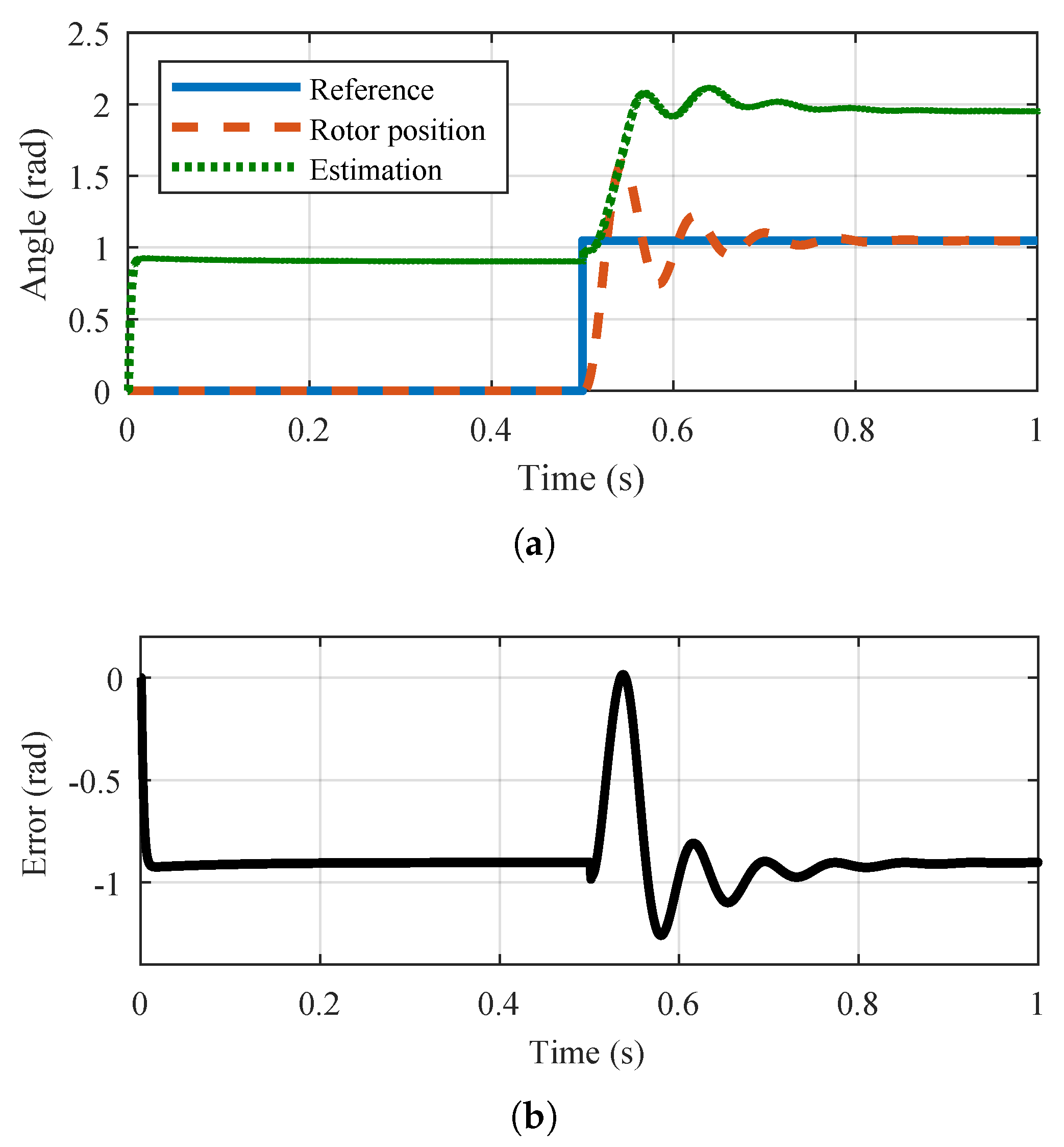
4. Simulation Results

For validating the use of both components, simulations tests are conducted. A fixed position of the rotor is selected by applying a constant voltage in the d axis. This voltage is transferred to the stator frame using a reference angle. The rotor will align itself with this reference and the tracking can be observed. This situation can be depicted in Figure 4 for the traditional demodulation scheme from Figure 2. In Figure 4a it can be observed that this scheme converges to the wrong value, maintaining this error through the test. Next, the same condition is applied to the case where both signals, negative and positive sequence, are used. This can be observed in Figure 5, were both signals are represented. Both waveforms are identical and present the same errors in magnitude, but opposite signs (Figure 5a). Using the proposed scheme presented in Figure 3, the black dashed-dotted signal is obtained. As it can be seen from Figure 5b, the rotor position estimated in this case has no error.
In order to validate the scheme proposed, a more complete simulation is conducted. A closed loop FOC is implemented to test the dynamic behavior of the estimation. The signal flow for the estimation procedure used in Figure 3 is shown in Figure 6. The voltage injection can be observed in Figure 6a and detailed in Figure 6b. Figure 6c shows both the voltage and the phase current and i c S , separated by a BPF. These two waveforms are better depicted in the magnified version of Figure 6c. The carrier current is then processed to obtain the positive and negative sequence of the signals, whose real parts are depicted in Figure 6e. In the detailed version of these components (Figure 6f) it can be observed how both components are identical with different sign. This components are fed to the controllers and their outputs combined, to form the estimated speed, which can be observed in Figure 6g. It is interesting to note here how the opposite signs already discussed can help to attenuate the ripple and provide a more accurate result, as it can be observed in the magnified Figure 6h.

5. Signal Processing

In order to improve accuracy of the speed and angle estimation, the measured currents should be filtered using analog filters to eliminate aliasing effects. Another source of error in the estimation will be the phase lag due to this filtering as well as computation and sampling lags.

5.1. Filtering

As stated before, aliasing of the high frequency noise coming from the inverter could deteriorate the quality of the estimation. In order to avoid this, an analog first order LPF combined with a voltage buffer will be used. The aim of the buffer is to decouple the filter from the analog input channel of the control platform.
For the separation of the carrier current from the line current, a second order butterworth BPF is digitally implemented in the control system. This filter is made up of two second order LPF and High Pass Filter (HPF). Although the injection is done at ω c , from (2) it can be seen that the currents will not be located exactly at the same frequency. Therefore, the cut-off frequencies for the LPF and HPF are separated 200 Hz to allow a good recovery of the signal.

5.2. Lag Compensation

The filtering as well as other lags related to analog to digital converters will introduce an important error in the angle estimation that would render the system unstable. Several studies have reported this effect which is very dependent on the characteristics of each system and the observer employed [25,26]. In this study, a more empirical approach has been followed, trying to relate the error observed in the estimation with the speed of the machine.
Using the demodulation algorithm depicted in Figure 3, the position estimation is calculated while running the machine using a resolver. The difference between the real angle and the estimated one is shown as the error signal of Figure 7. It can be clearly observed that there is a linear relationship between these two variables, due to filter lags and computation delays. The estimated mechanical position of the rotor, θ ^ , can then be expressed as
θ ^ = δ ^ p + e ( ω r ) δ ^ p + k 1 ω r e f + k 0 ,
where p are the pole pairs and k 0 , k 1 the regression coefficients from the data represented by Figure 7. In order to simplify the computation and avoid introducing another algebraic loop, the speed reference is used for the calculation of the compensation rather than the measured speed of the rotor. This lag compensation is only applied to the proposed control scheme since the traditional one exhibits a convergence problem that does not allow to operate in full sensorless mode.

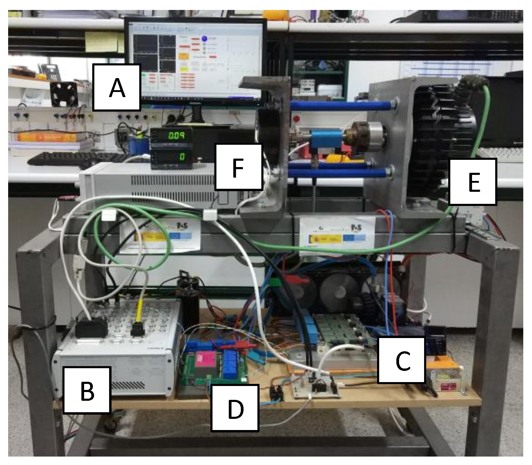
6. Experimental Results

The traditional and proposed algorithms have been coded in Matlab Simulink and built into a dSPACE MicroLabBox control platform. The host PC runs ControlDesk and FOC is used to control the motor speed and torque. The main control scheme is depicted in Figure 8. According to (1), the voltage injection is made in the real axis of the estimated rotor frame. Pulse Width Modulation (PWM) is then used to generate the signals for controlling the IGBTs in the inverter. The currents are measured and separated into fundamental and carrier terms by means of a BPF. The fundamental components are transferred to the rotor reference frame, having the high frequency content removed from the real component as it would interfere with the FOC. The carrier term is demodulated using the algorithms described. The experimental setup can be observed in Figure 9 and the main parameters of the system are summarized in Table 2. The controllers used for estimating the rotor angle are PI controllers. The tuning of these controllers has to be done taking into consideration that this position observer should be much faster than the speed control of the machine. For this work, Reference [27] has been used as the starting point for the PI design followed by manual tuning of the controllers.

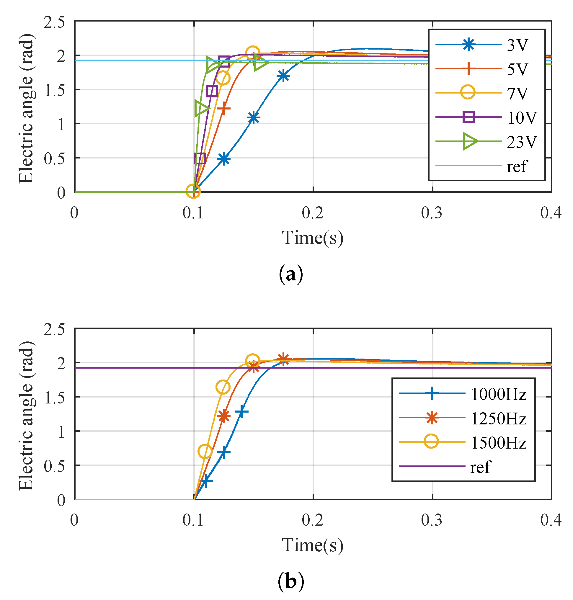
6.1. Frequency and Amplitude Voltage Selection

For determining the limits of operation of the proposed sensorless scheme, some preliminary tests are conducted. In the Figure 10 the rise time using the proposed algorithm for different levels of injection amplitude and frequency are represented. From this plot, the point (5 V, 1500 Hz) is selected as a candidate in the following tests. The Figure 11 shows the rotor position estimation as a function of the voltage and frequency used. In Figure 11a different amplitudes for the injection are tried while maintaining the frequency fixed at 1500 Hz, going up to a injection level of 10 % of the rated voltage of the machine. It can be observed that as the voltage increases, so will the convergence speed. However, since the voltage level is a trade-off between system bandwidth and noise and vibrations introduced in the system, 5 V is confirmed as a good option. Next, in Figure 11b different injection frequencies are tried out while keeping the voltage at 5 V, finally selecting 1500 Hz for its superior response. Since higher frequencies would compromise the reconstruction of the signal, given the sampling frequency, the injection parameters are fixed for the remaining tests as 5 V at 1500 Hz.

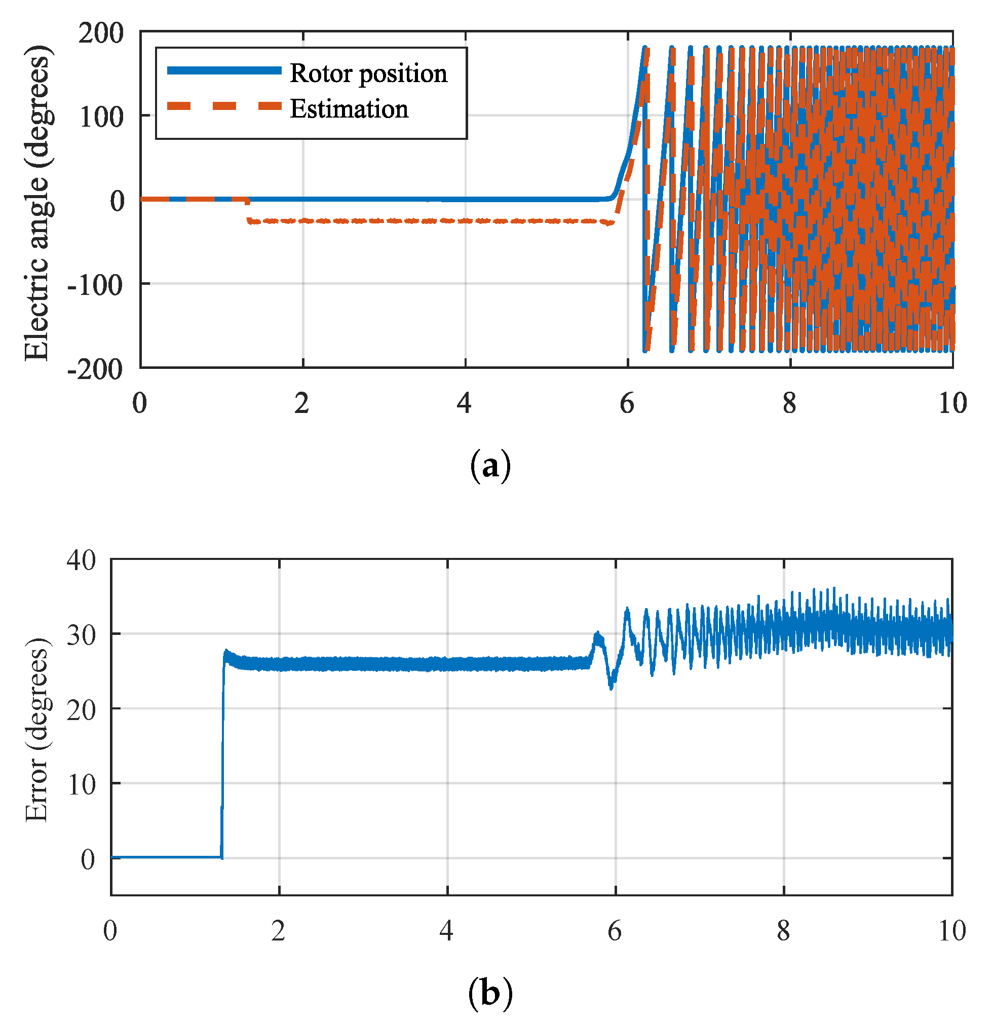
6.2. Comparison of Traditional and Proposed Demodulation Scheme

Moving on to the experimental tests, the two schemes are going to be compared. In this tests, only the filtering explained in Section 5.1 is going to be used. First the traditional demodulation schemed is executed. The motor is controlled using the resolver angle for the FOC. The estimated value of the rotor position is then compared to the measured one. These results are shown in Figure 12. First, the control is turned and afterwards, a speed reference of 200 rpm is set. Although it can be seen from Figure 12c that the speed estimation is correct, in Figure 12a,b a huge error is present when the machine starts and later on. This error would not allow the FOC to work properly if the estimated value were to be used.
Secondly, the proposed demodulation scheme is executed, again using the resolver angle for the FOC and comparing the results, which are shown in Figure 13. The same procedure is carried out, this time the speed estimations works also as expected, as shown in Figure 13c. Moreover, the error observed in the traditional scheme is eliminated, as can be seen in Figure 13a,b. The remaining small error is dependent on the speed and will be corrected as explained in Section 5.2.

6.3. Full Sensorless Mode

For the remaining tests, the estimation angle is going to be used for the FOC, so the machine will be operating in sensorless mode. The resolver angle will also be measured, but this time only for monitoring purposes. Also, the compensation described in (8) is applied, using the parameters from Table 2, that allows to compensate the error as shown in Figure 14. All the following tests use self-starting and the procedure is conducted as follows: before starting the motor, the rotor is fixed to the positive direction of the d-axis using the resolver. A positive and constant voltage is applied to the d-axis in order to be sure that the positive direction is identified (the detection of the d-axis using estimation techniques for the starting procedure is out of the scope of this paper). After that, the high frequency injection is turned on and only the estimated angle will be used for controlling the motor. The rotor is then kept still with a speed reference of 0 rpm. Finally, the motor is started setting a speed reference.
The results for the first test are presented in Figure 15, where the motor is started from still up to a 200 rpm speed. From Figure 15b, it can be seen that the system is able to operate and follows the speed reference. Afterwards, a negative speed reference is set and the zero crossing is tested. It can be seen from Figure 15a that some oscillations are observed, but the system is able to operate. These oscillations could be avoided if a higher voltage injection were to be used, but the authors tried to keep at the minimum to make it functional. With the injection used, the system is able to do self starting even loaded, as it will be shown in following experiments.
To test the load capability, in the final test showed in Figure 16 a step load of 10 N·m is applied to the motor. From Figure 16a showing the i q current and Figure 16b showing the rotor speed, it can be verified the correct functioning of the system under heavy loading. Moreover, to explore the limits of operation, start up of the motor with different speed reference are conducted, reaching a lower limit of only 50 rpm, as shown in Figure 17. The experiments are also conducted while loading the machine, showing the ability of the control proposed to operate even in such limit conditions.

7. Conclusions

To summarize, an enhanced demodulation scheme has been developed and implemented successfully in an experimental platform for validation. The following may be concluded from this work:
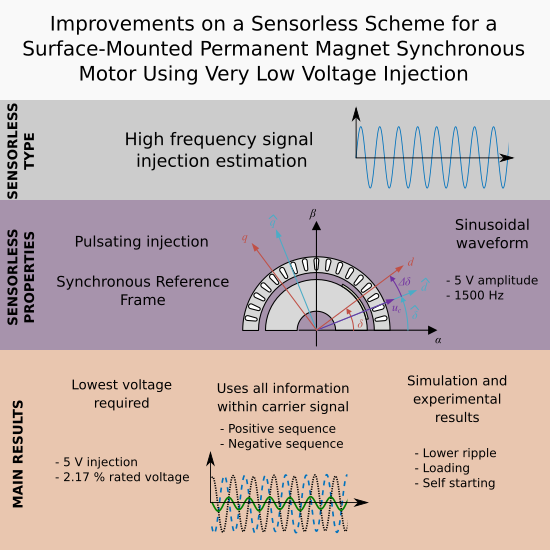
  • As it was stated in Section 2, the amplitude of the voltage injected greatly affects the performance of the sensorless algorithm. In the approach proposed, only 5 V was needed for the algorithm to work, which represents only a 2.17% of the rated voltage of the machine under test. Higher values could render better results, but at the expense of louder noise, vibrations and losses. Similarly, the frequency injection was chosen so to maximize the bandwidth of the FOC controllers while achieving good resolution given the sampling time.
  • The proposed demodulation method using all the information contained in the signal recovered provides far better results than the traditional scheme found in the literature. As commented in Section 3, given the frequency content of the two signals used, they compensate for errors and ripple produced from unwanted content during the processing. Simulation and experimental results validate the improvement achieved with the proposed algorithm. Nevertheless, the use of both sequences means extra computational effort for the microcontroller that could render the system unusable in systems with lower specifications.

Author Contributions

Conceptualization J.P.-A., E.R.-C., M.I.M.-M. and F.B.-G.; software J.P.-A.; methodology J.P.-A., E.R.-C.; investigation J.P.-A. and E.R.-C.; data curation J.P.-A.; visualization J.P.-A.; writing—original draft preparation J.P.-A.; writing—review and editing E.R.-C., M.I.M.-M. and F.B.-G.; supervision E.R.-C. and M.I.M.-M.; project administration, F.B.-G.; funding acquisition, E.R.-C. and F.B.-G. All authors have read and agreed to the published version of the manuscript.

Funding

This work was supported by the Junta de Extremadura (Regional Government) predoctoral researchers formation plan (PD16044).

Conflicts of Interest

The authors declare no conflict of interest. The funders had no role in the design of the study; in the collection, analyses, or interpretation of data; in the writing of the manuscript, or in the decision to publish the results.

Abbreviations

The following abbreviations are used in this manuscript:
SStator reference frame
u c Voltage injected
i c High frequency current
i p Filtered high frequency current
U c Amplitude of the voltage injected
ω c Angular frequency of the signal injected
jImaginary unit
δ Rotor angle (electrical radians)
δ ^ Estimated rotor angle (electrical radians)
Δ δ Error committed in the estimation
l d , l q Direct and quadrature inductances
θ ^ Estimated rotor angle (mechanical radians)
pPole pairs
k 0 , k 1 Linear regression coefficients
ω r e f Mechanical speed reference
f c Cut-off frequency

References

  1. Yan, Y.; Wang, S.; Xia, C.; Member, S.; Wang, H.; Shi, T. Hybrid Control Set-Model Predictive Control for Field-Oriented Control of VSI-PMSM. IEEE Trans. Energy Convers. 2016, 31, 1622–1633. [Google Scholar] [CrossRef]
  2. Wang, Z.; Chen, J.; Cheng, M.; Chau, K.T. Field-oriented control and direct torque control for paralleled VSIs Fed PMSM drives with variable switching frequencies. IEEE Trans. Power Electron. 2016, 31, 2417–2428. [Google Scholar] [CrossRef]
  3. Lara, J.; Xu, J.; Chandra, A. Effects of Rotor Position Error in the Performance of Field-Oriented-Controlled PMSM Drives for Electric Vehicle Traction Applications. IEEE Trans. Ind. Electron. 2016, 63, 4738–4751. [Google Scholar] [CrossRef]
  4. Anuchin, A.; Astakhova, V.; Shpak, D.; Zharkov, A.; Briz, F. Optimized method for speed estimation using incremental encoder. In Proceedings of the 19th International Symposium on Power Electronics (Ee), Novi Sad, Serbia, 19–21 October 2017; pp. 1–5. [Google Scholar] [CrossRef]
  5. Holtz, J. Sensorless Control of Induction Machines—With or Without Signal Injection? IEEE Trans. Ind. Electron. 2006, 53, 7–30. [Google Scholar] [CrossRef] [Green Version]
  6. Bojoi, R.; Pastorelli, M.; Bottomley, J.; Giangrande, P.; Gerada, C. Sensorless control of PM motor drives—A technology status review. In Proceedings of the 2013 IEEE Workshop on Electrical Machines Design, Control and Diagnosis (WEMDCD), Paris, France, 11–12 March 2013; pp. 168–182. [Google Scholar] [CrossRef]
  7. Zhang, G.; Wang, G.; Xu, D. Saliency-Based Position Sensorless Control Methods for PMSM Drives—A Review. Chin. J. Electr. Eng. 2017, 3, 14–23. [Google Scholar]
  8. Lee, D.; Akatsu, K. The study on transient performance improvement of position sensorless control algorithm for IPMSM. In Proceedings of the 2017 8th International Symposium on Sensorless Control for Electrical Drives (SLED), Catania, Italy, 18–19 September 2017; pp. 67–72. [Google Scholar] [CrossRef]
  9. Lindemann, G.; Weber, B.; Mertens, A. Reducing the Low-Speed Limit for Back-EMF Based Self-Sensing Speed Control by Using an FPGA-Operated Dead-Time Compensation. In Proceedings of the 2018 IEEE 9th International Symposium on Sensorless Control for Electrical Drives (SLED), Helsinki, Finland, 3–14 September 2018; pp. 60–65. [Google Scholar]
  10. Bao, D.; Pan, X.; Wang, Y.; Wang, X.; Li, K. Adaptive Synchronous-Frequency Tracking-Mode Observer for the Sensorless Control of a Surface PMSM. IEEE Trans. Ind. Appl. 2018, 54, 6460–6471. [Google Scholar] [CrossRef]
  11. Linke, M.; Member, S.; Kennel, R.; Member, S.; Holtz, J. Sensorless position control of Permanent Magnet Synchronous Machines without Limitation at Zero Speed. In Proceedings of the IEEE 2002 28th Annual Conference of the Industrial Electronics Society, IECON 02, Sevilla, Spain, 5–8 November 2002. [Google Scholar]
  12. Briz, F.; Degner, M.W.; García, P.; Lorenz, R.D. Comparison of saliency-based sensorless control techniques for AC machines. IEEE Trans. Ind. Appl. 2004, 40, 1107–1115. [Google Scholar] [CrossRef]
  13. Holtz, J. Acquisition of position error and magnet polarity for sensorless control of PM synchronous machines. IEEE Trans. Ind. Appl. 2008, 44, 1172–1180. [Google Scholar] [CrossRef]
  14. Xu, P.; Zhu, Z. Novel Carrier Signal Injection Method Using Zero Sequence Voltage for Sensorless Control of PMSM Drives. IEEE Trans. Ind. Electron. 2016, 63, 2053–2061. [Google Scholar] [CrossRef]
  15. Degner, M.W.; Lorenz, R.D. Position Estimation in Induction Machines Utilizing Signal Injection. IEEE Trans. Ind. Appl. 2000, 36, 736–742. [Google Scholar] [CrossRef] [Green Version]
  16. Trancho, E.; Ibarra, E.; Arias, A.; Salazar, C.; Lopez, I.; Diaz De Guereñu, A.; Peña, A. A novel PMSM hybrid sensorless control strategy for EV applications based on PLL and HFI. In Proceedings of the IECON Proceedings (Industrial Electronics Conference), Florence, Italy, 23–26 October 2016; pp. 6669–6674. [Google Scholar] [CrossRef] [Green Version]
  17. García, P.; Briz, F.; Degner, M.W.; Díaz-Reigosa, D. Accuracy and bandwidth limits of carrier signal injection-based sensorless control methods. In Proceedings of the Conference Record of the 2006 IEEE Industry Applications Conference Forty-First IAS Annual Meeting, Tampa, FL, USA, 8–12 October 2006; Volume 2, pp. 897–904. [Google Scholar] [CrossRef]
  18. Hwang, C.E.; Lee, Y.; Sul, S.K. Analysis on the position estimation error in position-Sensorless operation using pulsating square wave signal injection. IEEE Trans. Ind. Appl. 2019, 55, 844–850. [Google Scholar] [CrossRef]
  19. Kim, S.I.; Im, J.H.; Song, E.Y.; Kim, R.Y. A New Rotor Position Estimation Method of IPMSM Using All-Pass Filter on High-Frequency Rotating Voltage Signal Injection. IEEE Trans. Ind. Electron. 2016, 63, 6499–6509. [Google Scholar] [CrossRef]
  20. Tang, Q.; Shen, A.; Luo, X.; Xu, J. PMSM Sensorless Control by Injecting HF Pulsating Carrier Signal into ABC Frame. IEEE Trans. Power Electron. 2017, 32, 3767–3776. [Google Scholar] [CrossRef]
  21. Ni, R.; Xu, D.; Blaabjerg, F.; Lu, K.; Wang, G.; Zhang, G. Square-wave voltage injection algorithm for PMSM position sensorless control with high robustness to voltage errors. IEEE Trans. Power Electron. 2017, 32, 5425–5437. [Google Scholar] [CrossRef]
  22. Xie, G.; Lu, K.; Dwivedi, S.K.; Rosholm, J.R.; Blaabjerg, F. Minimum-Voltage Vector Injection Method for Sensorless Control of PMSM for Low-Speed Operations. IEEE Trans. Power Electron. 2016, 31, 1785–1794. [Google Scholar] [CrossRef]
  23. Xu, P.; Zhu, Z. Carrier signal injection-based sensorless control for permanent magnet synchronous machine drives with tolerance of signal processing delays. IET Electr. Power Appl. 2017, 11, 1140–1149. [Google Scholar] [CrossRef]
  24. Luo, X.; Tang, Q.; Shen, A.; Zhang, Q. PMSM Sensorless Control by Injecting HF Pulsating Carrier Signal into Estimated Fixed-Frequency Rotating Reference Frame. IEEE Trans. Ind. Electron. 2016, 63, 2294–2303. [Google Scholar] [CrossRef]
  25. Lin, T.C.; Zhu, Z.Q. Sensorless operation capability of surface-mounted permanent-magnet machine based on high-frequency signal injection methods. IEEE Trans. Ind. Appl. 2015, 51, 2161–2171. [Google Scholar] [CrossRef]
  26. Moghadam, M.A.G.; Tahami, F. Sensorless control of PMSMs with tolerance for delays and stator resistance uncertainties. IEEE Trans. Power Electron. 2013, 28, 1391–1399. [Google Scholar] [CrossRef]
  27. Jin, X.; Ni, R.; Chen, W.; Blaabjerg, F.; Xu, D. High-Frequency Voltage-Injection Methods and Observer Design for Initial Position Detection of Permanent Magnet Synchronous Machines. IEEE Trans. Power Electron. 2018, 33, 7971–7979. [Google Scholar] [CrossRef]
Figure 1. Phasor diagram for the high frequency voltage injection.
Energies 13 02732 g001
Figure 2. Demodulation scheme for the traditional algorithm.
Energies 13 02732 g002
Figure 3. Proposed demodulation scheme using also the negative sequence current.
Energies 13 02732 g003
Figure 4. Simulation results using the traditional demodulation scheme. (a) Reference angle (blue solid), rotor position (dashed orange), estimated angle (dotted green). (b) Estimation error.
Energies 13 02732 g004
Figure 5. Simulation results extracting both components. (a) Reference angle (blue solid), rotor position (dashed orange), estimated angle (dotted green) from positive sequence, estimated angle (dotted purple) from negative sequence, estimated angle (dash-dot black) using both signals. (b) Estimation error.
Energies 13 02732 g005
Figure 6. Simulations results for the estimation procedure of the proposed demodulation scheme. (a) d axis voltage reference. (b) Magnified waveform of (a). (c) Phase current (dotted blue) and carrier current (solid orange). (d) Magnified waveform of (c). (e) Real parts of the positive (blue) and negative (orange) sequences. (f) Magnified waveforms of (e). (g) Positive sequence (dashed blue), negative sequence (dotted orange) and composed (solid green) speeds. (h) Magnified waveforms of (g).
Energies 13 02732 g006
Figure 7. Error committed in the position estimation for different rotor speeds. Angle error expressed in mechanical radians.
Energies 13 02732 g007
Figure 8. Control and demodulation scheme used for experimental procedure.
Energies 13 02732 g008
Figure 9. Experimental setup. (A) Host machine. (B) Target platform. (C) IGBT inverter. (D) Measuring stage. (E) Surface Mounted Permanent Magnet Synchronous Motor (SMPMSM). (F) Electromagnetic brake.
Energies 13 02732 g009
Figure 10. Response time measured for different amplitude and frequency injections.
Energies 13 02732 g010
Figure 11. Injection voltage and frequency selection procedure. (a) Different voltage levels for a 1250 Hz frequency injection. (b) Different frequency levels for a 5 V amplitude injection.
Energies 13 02732 g011
Figure 12. Experimental results using the traditional demodulation scheme. (a) Real (solid blue) and estimated (dashed orange) angles. (b) Estimation error. (c) Reference (dashed yellow), measured (dotted orange) and estimated (solid blue) speeds.
Energies 13 02732 g012aEnergies 13 02732 g012b
Figure 13. Experimental results using the proposed demodulation scheme. (a) Real (solid blue) and estimated (dashed orange) angles. (b) Estimation error. (c) Reference (dashed yellow), measured (dotted orange) and estimated (solid blue) speeds.
Energies 13 02732 g013
Figure 14. Angle compensation for the motor running at 200 rpm.
Energies 13 02732 g014
Figure 15. Start-up of the motor only using the estimated position and speed. (a) Estimation error. (b) Reference (dashed yellow), measured (dotted orange) and estimated (solid blue) speeds.
Energies 13 02732 g015aEnergies 13 02732 g015b
Figure 16. Loading of the motor only using the estimated position and speed. (a) i q current. (b) Reference (dashed yellow), measured (dotted orange) and estimated (solid blue) speeds.
Energies 13 02732 g016
Figure 17. Start up of the motor for three different speeds, from top to bottom 150, 100 and 50 rpm. On the left column the motor is not loaded and in the right column, the load is applied. Reference (dashed yellow), measured (dotted orange) and estimated (solid blue) speeds.
Energies 13 02732 g017
Table 1. Different injection levels found in the literature.
ReferenceVoltage Injection% of Rated Voltage
[26]100 V78.74
[18]40 V66.6
[22]45 V56.25
[21]30 V40.65
[19]40 V33.33
[23]45 V28.48
[14]4 V11.11
[24]20 V9.09
[20] 7.75 V3.52
Table 2. Main parameters of the system.
ParameterValueUnits
Sampling frequency10kHz
Switching frequency10kHz
Injection voltage5V
Injection frequency1500Hz
Analog LPF f c 3.2kHz
d current loop digital LPF f c 500Hz
Estimator LPF f c 500Hz
Estimation compensation coefficient k 0 0.0083-
Estimation compensation coefficient k 1 0.0091-
DC bus voltage100V
PMSM rated power6700W
Rated voltage230V
Rated speed3000rpm
Rated torque at 3000 rpm 22.53 N·m
Rated current at 3000 rpm23.7 AA
Stator resistance 0.7 Ω
direct axis inductance 0.001871 H
quadrature axis inductance 0.001616 H
Magnet flux 0.1323 V·s/rad
Rotor inertia 0.0036 kg·m 2
Viscous friction coefficient 0.1323 N·m·s
Pole pairs4-

