Evaluation of Photovoltaic and Battery Storage Effects on the Load Matching Indicators Based on Real Monitored Data

Abstract

This paper reports on the electrical performance of two bloc-of-flats buildings located in Prague, Czech Republic. Measured data of electrical consumption were used to investigate the effect of photovoltaic (PV) and battery energy storage system (BESS) systems on the overlap between generation and demand. Different PV array configurations and battery storage capacities were considered. Detailed solar analysis was carried out to analyze the solar potential of the building and to assess the PV electricity production. The evaluation of the building performance was done through MATLAB simulations based on one-year monitored data. The simulation results were used for the calculation of the load matching indices: namely, the self-consumption and self-sufficiency. It was found that optimized array tilt and orientation angles can effectively contribute to a better adjustment between electricity demand and solar PV generation. The addition of a façade PV system increases significantly the PV generation and thus the load matching during winter months. Mismatch is further reduced by using the energy flexibility provided by the BESS. Depending on the PV size and BESS capacity, the self-consumption and the self-sufficiency of the building could increase from 55% to 100% and from 24% up to 68%, respectively.

1. Introduction

The sudden growth and expansion of cities have caused a substantial increase in the energy consumption and carbon emissions. Statistics have shown that buildings are responsible for 40% of energy consumption and almost 38% of the greenhouse gases in the EU [1]. Currently, there is a major transformation taking place through national building codes, roadmaps, and plans for increasing the number of nearly zero-energy buildings (nZEB) [2]. Buildings need to be energy efficient and fully utilize renewable energy to supply the remaining low demand [3].

From this perspective, photovoltaics (PVs) could be the main technology to generate on-site electricity, satisfying part of buildings’ demand and to achieve net or nearly zero energy target. Many countries introduced subsidy schemes to promote the residential solar PV, the vast majority of each correspond to grid-connected systems. Generated electricity can be consumed instantly on-site or exported to the grid (net metering scheme). However, termination of the feed-in tariffs in many countries turned the attention of the researchers and PV system owners toward the self-consumption of on-site PV generated electricity [4].

Residential buildings, with PV systems operating under the net metering scheme, receive around 70% of their energy needs from the utility grid. From the studies surveyed by Luthander et al. [4], it appears that on average, 35% of electricity is self-consumed if no specific actions and/or investments are undertaken. Similar results were obtained by Gjorgievski et al. [5], who studied 55 Cypriot households with 3 kW_p rooftop PV generators. The self-consumption for 3 kW_p PV systems was found to be around 48%, while households with larger PV generators were characterized by lower load matching capabilities (self-consumption values around 19%). Conversely, results presented by [6] indicated that higher self-consumption for small PV systems (<10 kW) is a consequence of high electricity demand.

In this context, a better match between generation and consumption is needed to improve grid interaction and lower the stress on the electricity distribution grid [7]. Optimization of the PV installation can be used to shift the electricity generation according to the particular load profile [8]. Freitas et al. [9] analyzed how making use of the different tilts and orientation of surfaces in buildings contribute to a better adjustment between electricity demand, solar PV generation, and minimizing storage needs. Hence, it is important to select the PV configuration that maximizes the self-consumption. In a recent study, Mubarak et al. [10] found that East-West orientation resulted in a better self-consumption rate, while Southeast-Southwest (SE-SW) result in the highest degree of autarky compared to South orientation. This is particularly valid for the rooftop PV system—the most popular application in residential buildings—where adjustment of the tilt and azimuth angles could be easier compared to façade systems. On the other hand, façade PVs come in various configurations affecting not only the energy performance, but also the indoor comfort [11]. Even if they receive less irradiation compared to rooftop PVs, they produce relatively more power in winter as well as in the early and late hours of the day.

The battery energy storage system (BESS) is the key element of stable and secure supply of electricity as it can mitigate the volatility of Renewable Energy Sources (mainly PV and wind). There are various battery technologies available in the market suitable for residential application, for example lead-acid, lithium-ion (Li-ion), sodium-sulfur (NaS), nickel-cadmium (NiCd), and nickel metal hydride (NiMH) [12]. Lithium-ion (Li-ion) batteries are currently the benchmark technology for residential applications as well as for other stationary applications [13,14]. In addition to their enhanced lifetime and high storage efficiency, the overall price of Li-ion batteries (at the system level) has dropped by 20% p.a. since 2013, making them more attractive than traditional lead-acid batteries [15].The BESS can enhance the self-consumption of buildings from few percentages up to the theoretical maximum of 100%. Since battery storage costs also decreased strongly over recent years, considerable amounts of research on the improvement of PV self-consumption at residential buildings using a battery have been carried out [16,17,18]. In Luthander et al. [4], it was shown that a battery storage capacity of 0.5–1 kWh per installed kW_p PV power could increase the relative self-consumption by 13%–24% compared to the original rate. Some works focused on the optimal sizing of battery systems at building [7] or community scale [19,20]. In Kotarela et al. [21], a methodology was presented for the optimal sizing of the electrical storage, taking into account the impact on the operation of the utility grid.

Other studies were dedicated to provide insights into the techno-economic benefits of battery storage coupled to PV systems, where the authors assessed the sensitivities of the battery’s economic attractiveness to the capital expenditure and electricity prices [22,23,24,25]. Cucchiella et al. [26] proposed a mathematical model for the evaluation of the financial feasibility of the PV-BESS systems in Italy. They concluded that lead-acid technology can be profitable in the presence of subsidies. Based on real data acquired over a period of 12 months, Kosmadakis et al. [27] estimated that the cost of energy produced from a PV system combined with lead–acid batteries was 0.58 €/kWh. Conversely, Li-ion batteries could also become profitable in case of larger households and locations with high irradiance levels according to the study in [28].

Alternatively, some authors were interested on the combination of batteries with PVs in terms of providing some ancillary services to the grid, e.g., load–demand shifting [29,30], covering the peak capacity [31]. Solano et al. [32] introduced a model for the control of BESS considering strategies for increasing self-consumption and grid-peak-shaving. Finally, Liu et al. [33] performed a multi-criterion optimization considering the comprehensive technical, economic, and environmental performance indicators. The standard deviation of net grid power, battery cycling aging, and CO₂ emission were reduced by 3.4%, 78.5%, and 34.7%, respectively.

PV-BESS systems can play an important role in the transition toward a more sustainable power supply. The optimum design and control of such PV-BESS systems is still under investigation and represents a hot topic for various researchers. Thus, the present paper investigates the possible design solutions for adding PVs and BESS to a real monitored residential building based on its load profile. Performance assessment depends on time resolution and thus, high temporal resolution data were used, with a monitoring period starting from October 2018 to September 2019. The work analyzes the influence of different PV designs and BESS capacities on the load matching indices related to self-consumption and the self-sufficiency of the bloc-of-flats. Moreover, it highlights the importance of integrating PVs on the building façades for maximizing the overlapping between the load profile and the PV production.

The article is organized as follows: the description of the case study as well as the monitored load profiles data are provided in the next section. Section 3 details the employed methodology and models used for the evaluation of the performance of the case-study building. The relevant results are discussed in Section 4, and the conclusions are summarized in Section 5.

2. Case Study and Monitored Data

The present paper studies and investigates the possible solutions for adding photovoltaics (PVs) and battery energy storage system (BESS) to a building in order to increase the self-consumption of the energy generated locally. The investigation is carried out on two bloc-of-flats (houses) situated in suburban area (medium dense) of the city of Prague, Czech Republic. Prefabricated high-rise buildings built in the 1970s are characterized by a simple shape, flat roofs, and vertical façades with high fenestration ratio and balconies in two orientations. The buildings consist of 32 flats with 2761 m² of total heated area and have been refurbished recently. Thus, by following the same methodology developed in this work, buildings with similar monthly energy consumption and weather conditions will be able to generate and store their own produced energy and use it in an effective way.

The collection of data has been carried out based on a survey prepared for the owners and persons living in the two houses. The survey is based on some basic questions related to the topics given in

Table 1. Survey main questions.

People Count	Social Category and Activities	Appliances and Other
- Age, - Number of people, - Gender, - … etc.	- Seniors, - Kids, - Persons staying home, - Persons working outside, - Persons working from home, - Persons in parental leave, - … etc.	- Type of lighting, - TV type, - Electrical hoven, - Microwave, - PC, - … etc.

. The analysis of such data could reveal some interesting patterns about the behavior of some persons and how this behavior influences the energy consumption of the flat or the whole building.

More than 50% of flat owners (occupants) welcomed the survey and agreed to share their information. Figure 1 depicts the obtained data showing the percentage of flats owning the list of appliances listed in Table 1. It can be seen from the figure that the availability of appliances varies from one flat to another, and some basic appliances are available in all the flats.

Based on the analysis of the other data collected by the survey, the variation of the daily electricity consumption of each flat has been evaluated according to the number of appliances present and the number of people living in a flat. The left side of Figure 2 illustrates the effect of the number of electrical devices present in the flats on the energy consumption. The linear correlation trend shows that a high number of electrical devices leads to a high energy consumption; however, this is not always true, as there are flats with the same number of devices, but their daily energy consumption is very different. The right side of Figure 2 gives an idea about the influence of occupancy on the electrical consumption of the monitored flats. It can be seen from the figure that the flats’ occupancy varies from one to four people. The electricity consumption of the flats does not follow the occupancy rate, where it was found that flats with a lower number of occupants consume more energy than flats with a high number of occupants. The obtained R² values from the linear trend line show that is it hard to correlate the variation of the daily electricity consumption to the considered cases: the number of occupants and devices in the flat. The difficulty is mainly due to the behavior of the occupants, the age of the appliances (new or old technology), and to the limited amount of collected data. However, the only case that gives a better correlation to the increase of the electricity consumption is related to the number of appliances present inside the flat.

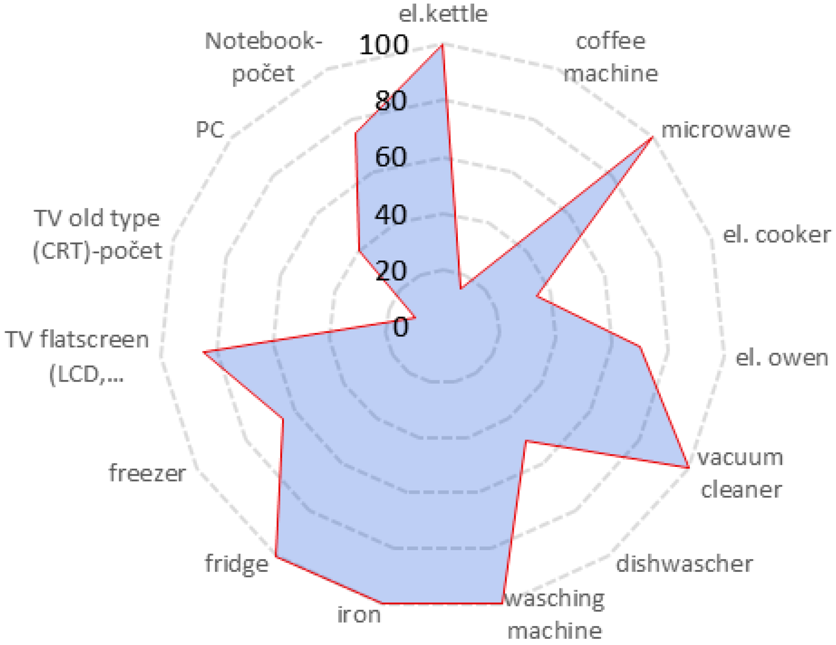
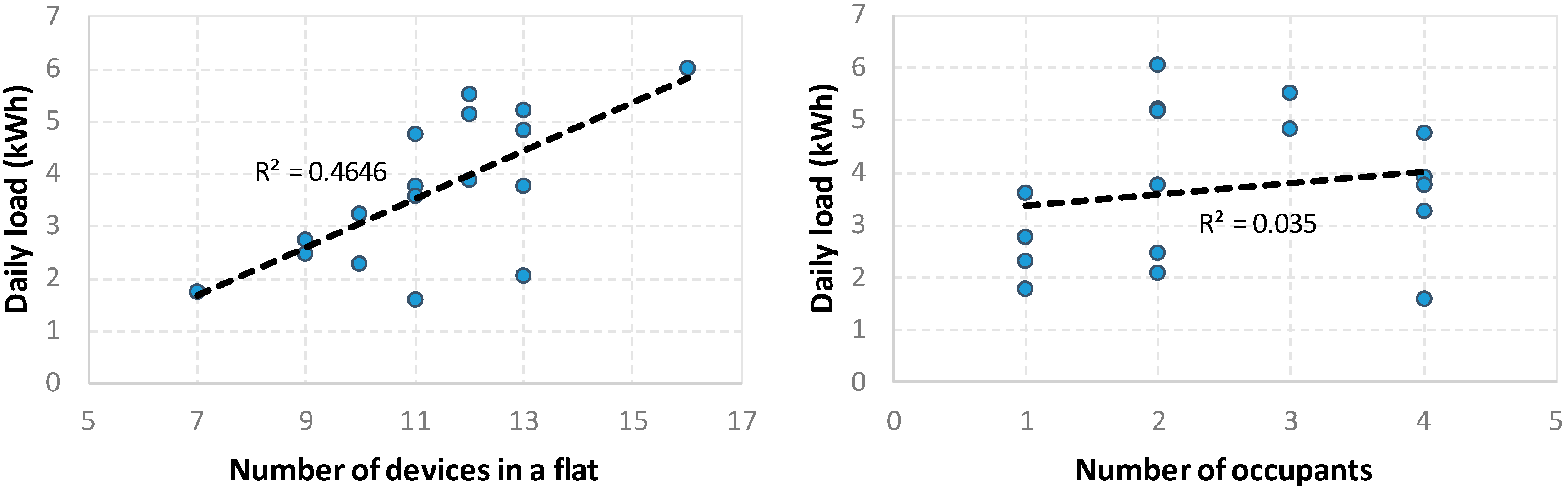
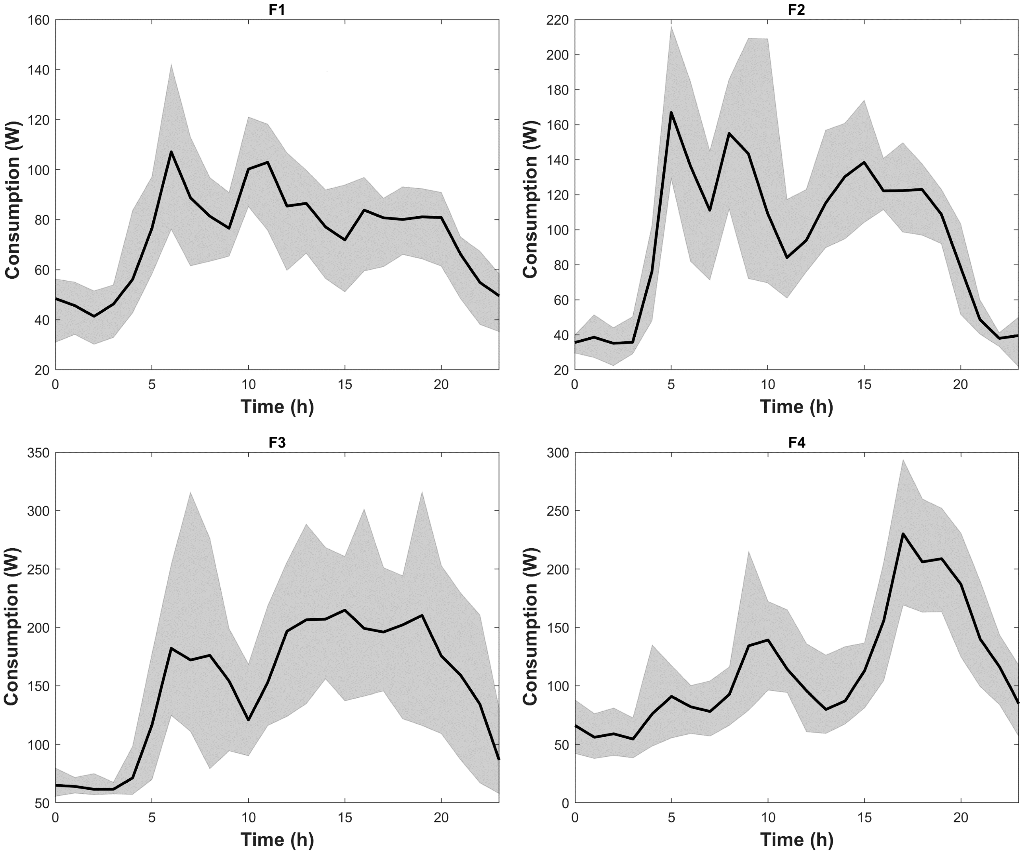
2.1. Consumption Profile Analysis

In addition to the survey, smart electricity meters were installed for monitoring the electricity profile of 17 flats (the flats corresponding to the owner who accepted to respond to the survey), as well as for the shared areas (corridors-lighting and elevator) and for each house separately. The electricity consumption data were monitored in one-minute timestep for a period ranging from October 2018 to September 2019. In order to have an accurate solar potential of the location, a Silicon Irradiance Sensors (Si-RS485TC) was installed on the roof of the building. The irradiance sensor was set up to measure the solar irradiance on horizontal plan and the ambient temperature in a one-minute timestep along the same monitored year.

In order to extract some typical electrical daily profiles, the data obtained from the energy meters have been analyzed according to the number of occupants (flats with one person, flats with two persons), and also for the common areas (corridor-lighting and elevator). The detailed analysis is given in the following paragraphs.

2.1.1. Flats with Single Person

There are four flats (F1, F2, F3, and F4) with a single person living inside. The first two flats (F1 and F2) have the same person profile (a pensioner woman living alone). The other flats correspond to one man working at home (F3) and the other one working outside (F4).

The comparison of the two flats F1 and F2 in terms of electricity consumption shows that F1 has a daily electrical energy consumption of 1.77 kWh, while the other flat F2 has a daily consumption of 2.29 kWh. The difference of energy consumption is mainly due to the electrical equipment present in each flat. There are 7 and 13 electrical devices in F1 and F2, respectively. Additional electrical devices such as the electric oven, PC, and freezer contribute to the higher load demand in F2.

The hourly load profiles of the flats F1 and F2 extracted from the measured data are given in the upper part of Figure 3. The gray surface in the graph represents the minimum and maximum variations of the consumption along the different months of the year. Meanwhile, the dark line represents the hourly average annual profile. It can be seen that the profile shape is almost the same for each flat, which means that the habits of the persons living inside are practically constant. However, the amplitude of the load power varies seasonally. In the winter period, the consumption is higher than in the summer period.

A daily electrical energy consumption of 3.59 kWh and 2.75 kWh was measured for the flats F3 and F4, respectively. The higher load demand in F3 can be attributed to the higher occupancy (home office) and additional appliances (electric oven) compared to F4. The lower part of Figure 3 depicts the daily profiles obtained. It can be clearly seen that for flat F3, the consumption of energy starts around 05:00 and during the whole day, and it remains fluctuating around certain values until 23:00. However, for flat F4, the load demand is during specific periods of the day. Here also, the typical profile of each flat is more or less similar to the monthly profiles; moreover, the seasonal variation can also be observed in both graphs related to F3 and F4.

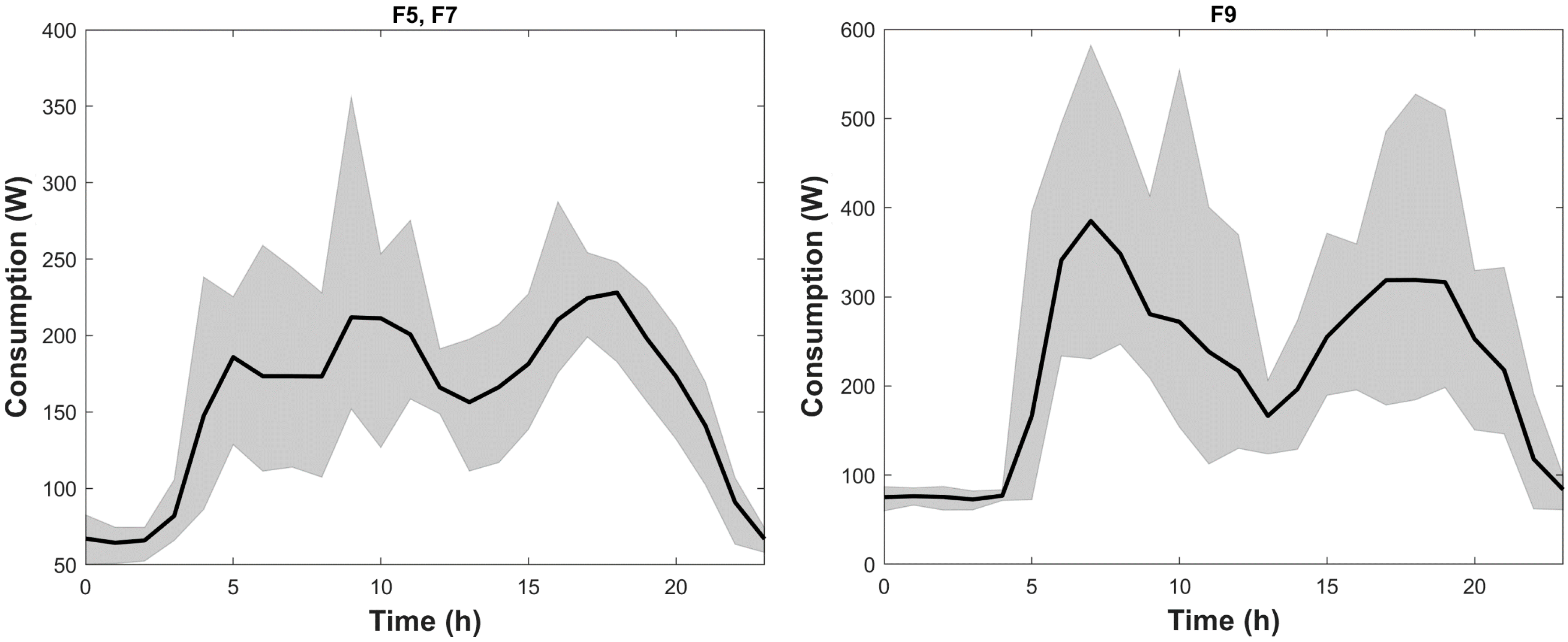
2.1.2. Flats with Two Persons

There are five flats with two persons living inside, four of which (F5, F6, F7, and F8) correspond to same people category (a couple of seniors). The fifth flat (F9) belongs to a young couple working outside. The daily electrical energy consumption of the flats F5, F6, F7, and F8 change according to the persons’ habits and the number of electrical devices present inside the flat. The shape of the daily load profiles shown in the left side of Figure 4 corresponds to flats F5 and F7. This consumption profile is pretty similar to the shape of the load profiles of flats F6 and F8, as these two flats accommodate people of the same age (seniors).

The daily load profiles related to flat F9 (persons working outside) are depicted in the right side of Figure 4. It can be seen that there are two periods where the load demand is high: the first is in the early morning (around 06:00) before going to work, and the second one is in the evening (around 19:00) after the return from work. Here also, it can be seen that the shape of the consumption profile is more or less the same for each flat and for the whole year. However, the amplitude of power varies according to the seasons, where higher consumption values occur in winter.

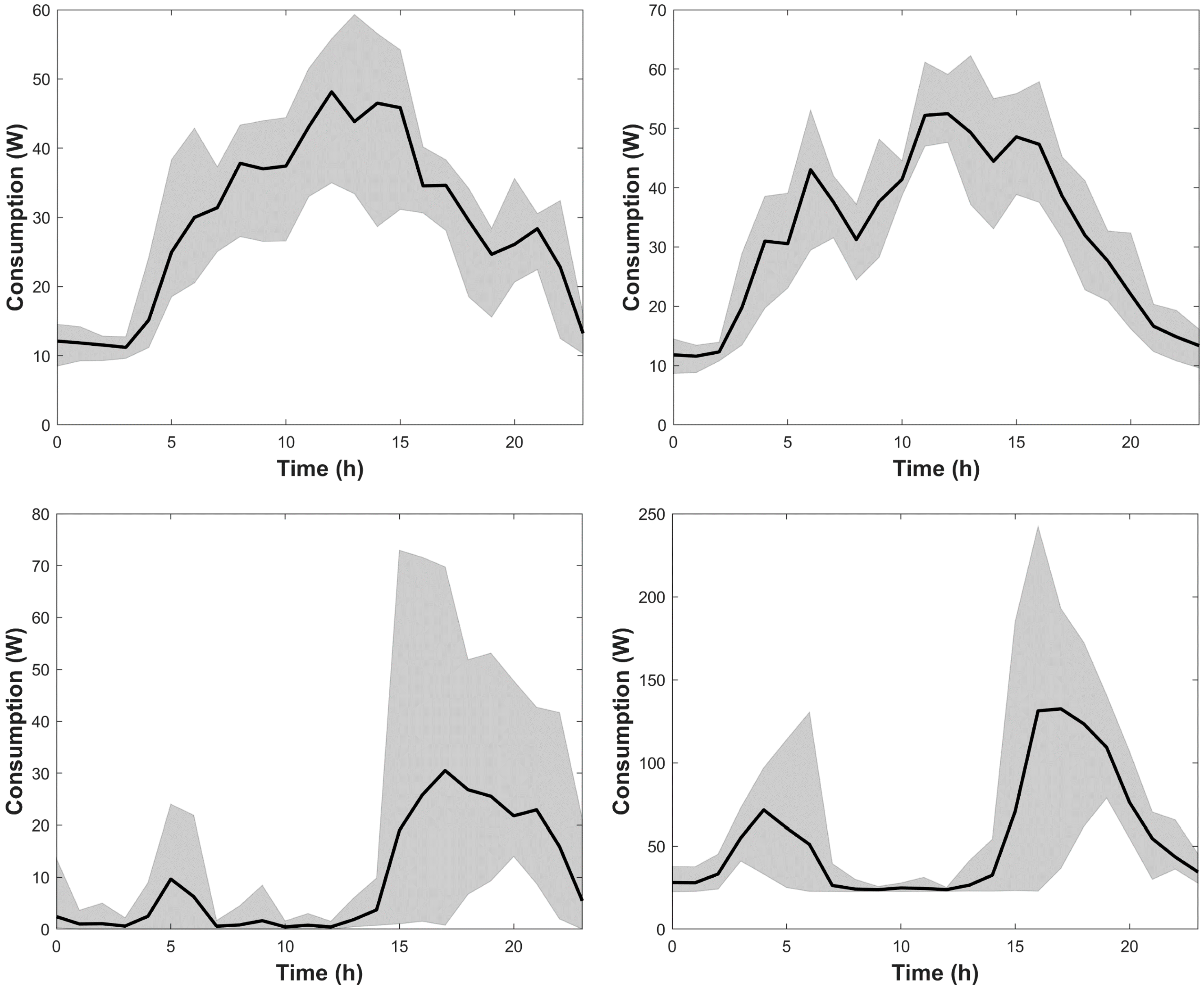
2.1.3. Common Space

The common space of the two houses was also monitored, and it represents the lighting energy consumption in the corridors and the consumption for the operation of the elevator. The upper part of Figure 5 highlights the elevator hourly consumption profiles in both houses. The gray surface in the graph represents the minimum and maximum variations of the consumption along the different months of the year. Meanwhile, the dark line represents the hourly average annual profile. It can be seen from Figure 5 that the hours of using the elevator are same for both houses, and the energy consumed is similar.

The lower part of Figure 5 shows the electrical energy consumed by the lighting in the two houses. It can be seen that the daily load profiles present the same shape for both houses. However, from the difference in the power magnitude, it can be concluded that the bulbs installed in the house corresponding to the data plotted in the right side of the lower part of Figure 5 consume more energy than the bulbs installed in the other house. In addition, there are some permanent loads or lights which are kept lit along the whole day.

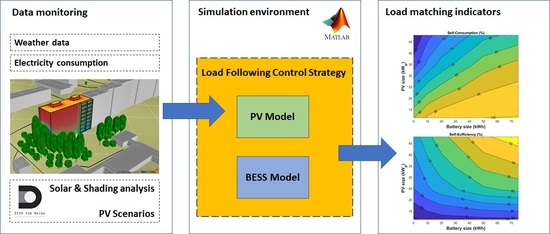
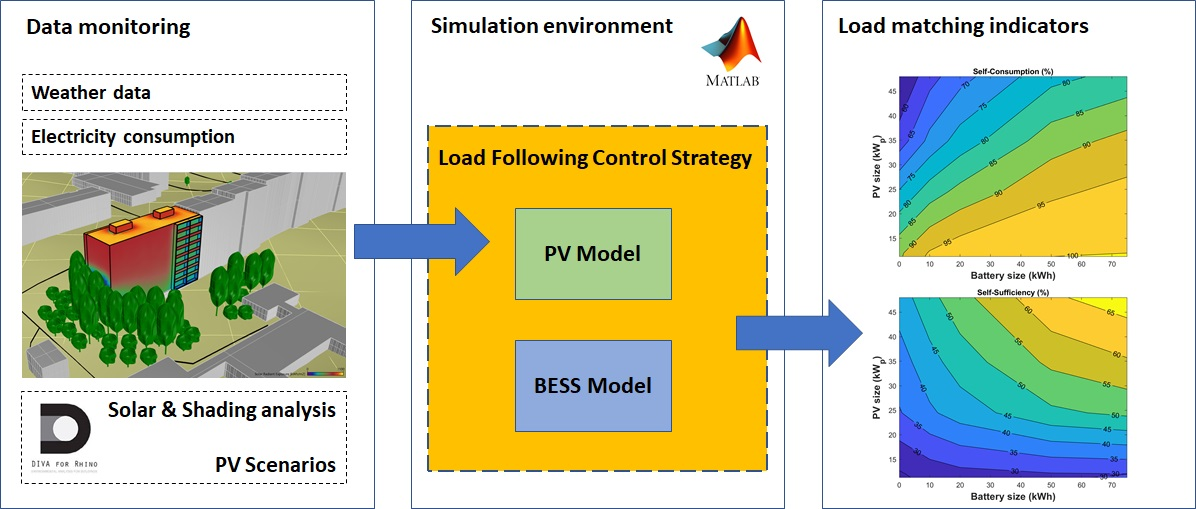
3. Methodology

This section describes the workflow of this study, along with all the data and tools used, variables of interest, and assumptions made. Section 3.1 and Section 3.2 describe the process for the solar radiation analysis on building surfaces and the PV scenarios considered in the study, respectively. Section 3.3 discusses the approach for the estimation of the electricity yield considering the environmental variables affecting the electrical efficiency of PV panels. Finally, details regarding the electricity storage modelling and the control strategy of the PV/BESS/Grid system are given in Section 3.4.

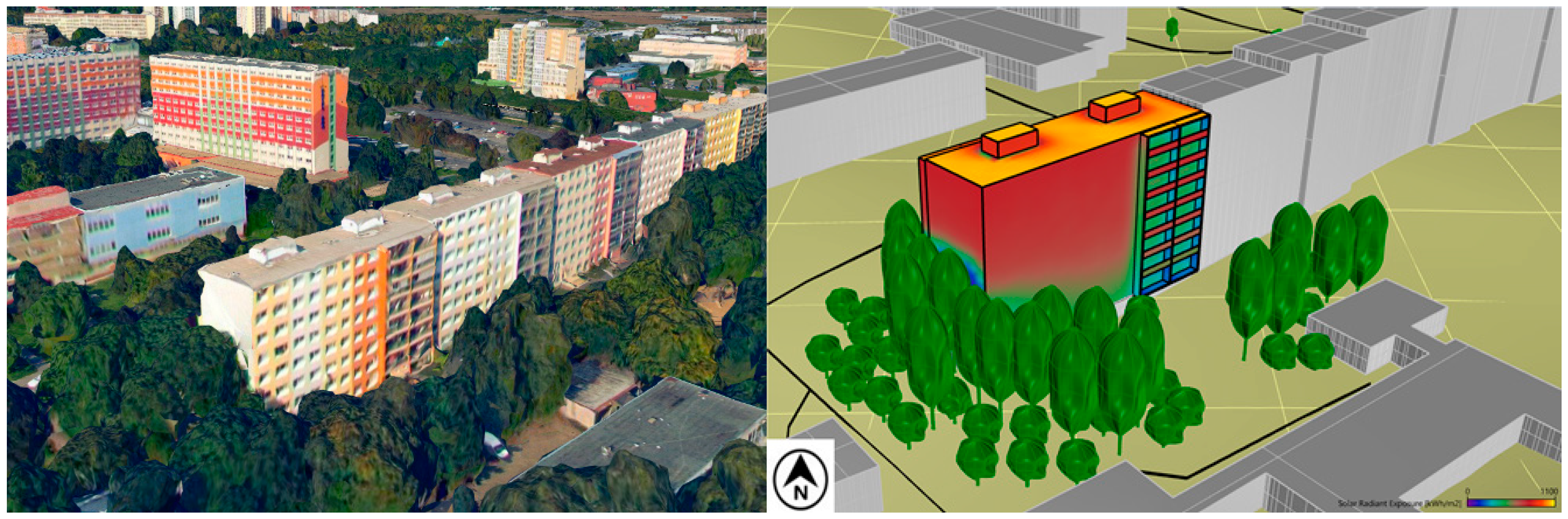
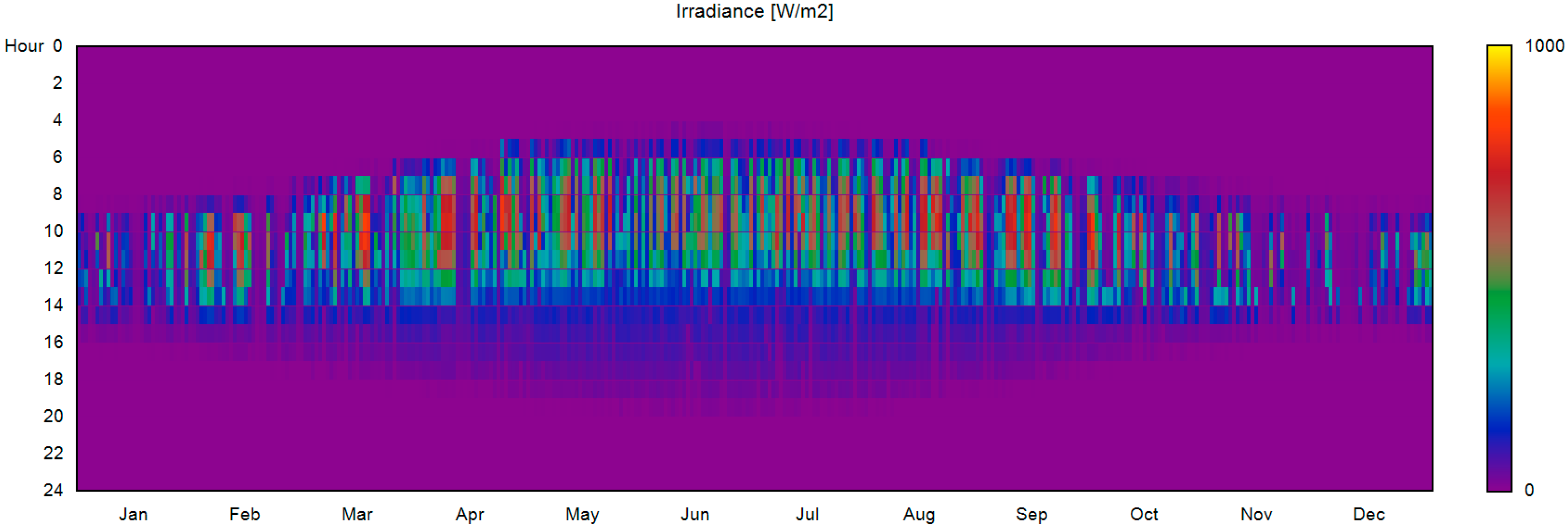
3.1. Solar Potential Analysis

In this study, a solar potential analysis was performed in Rhinoceros and its graphical algorithm editor plug-in Grasshopper. The 3D model of the building was prepared based on the actual architectural drawings, while façade elements (apart from balconies) were excluded. To take into account the effect from surrounding context, shadow casting elements, such as surrounding buildings and trees, were also imported using the Gismo plug-in [34]. Once the physical model is available, analysis was carried out in DIVA™ [35], a grasshopper plugin based on Radiance [36] and DAYSIM [37] simulation engines. It uses a daylight coefficient approach combined with the Perez all-weather sky model to predict the amount of solar radiation in buildings. Building, surfaces were divided according to the dimensions of the PV modules, forming a representative analysis grid. Each of these surfaces receives a different amount of solar radiation based on the orientation, tilt angle, and shadows or reflections from nearby objects. For this purpose, material properties have been associated with every building surface. The solar reflectance values of ground, facades, and roofs are set to 0.20, 0.35, and 0.30 respectively. Evaluation of the solar potential was made through the estimation of the annual irradiance (kWh/m²) according to the climatic data of the given location in Typical Meteorological Year (TMY) format.

The results are plotted on the 3D model on a false-color scale indicating the areas of the building envelope suitable for PV integration (Figure 6). These include the roof and part of vertical façades (shading effect) on SE and SW orientations. Rooftop PVs can be installed considering different inclination and/or orientation to obtain the desired generation profile, while vertical façades can support several Building-integrated Photovoltaic (BIPV) applications [11]. Suitable surfaces correspond to 70 m² on SW and 92 m² on SE façade (considering the actual fenestration ratio) respectively. Results obtained range between 660 and 770 kWh/m² for façades and can reach up to 1200 kWh/m² for the rooftop PV systems.

After selecting the suitable surfaces, detailed results regarding the irradiance values (W/m²) were collected for each PV module and imported to MATLAB^® environment for detailed PV modeling and estimation of the PV generation (described in the following subsection). An example of the simulated irradiance for a vertical integrated PV module is presented in Figure 7. As expected for an SE façade, a narrow irradiance profile is observed with peak values during the morning hours (maximum 840 W/m²).

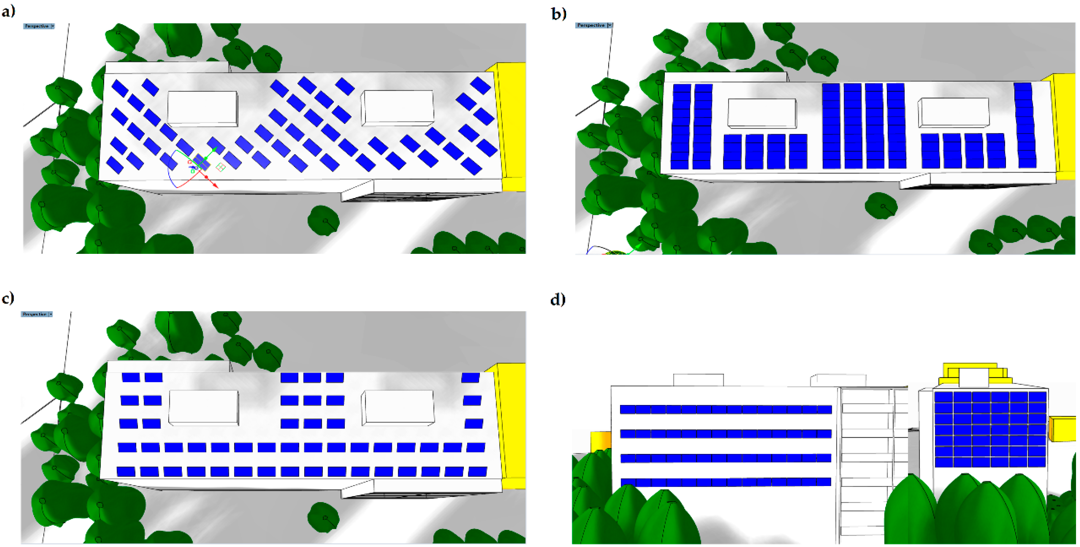
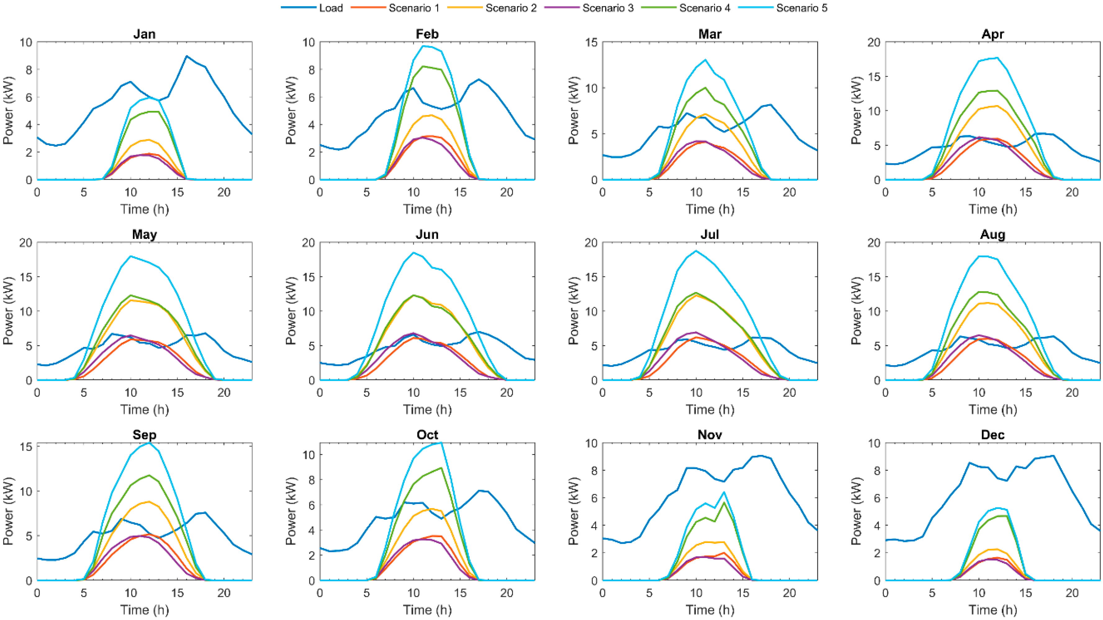
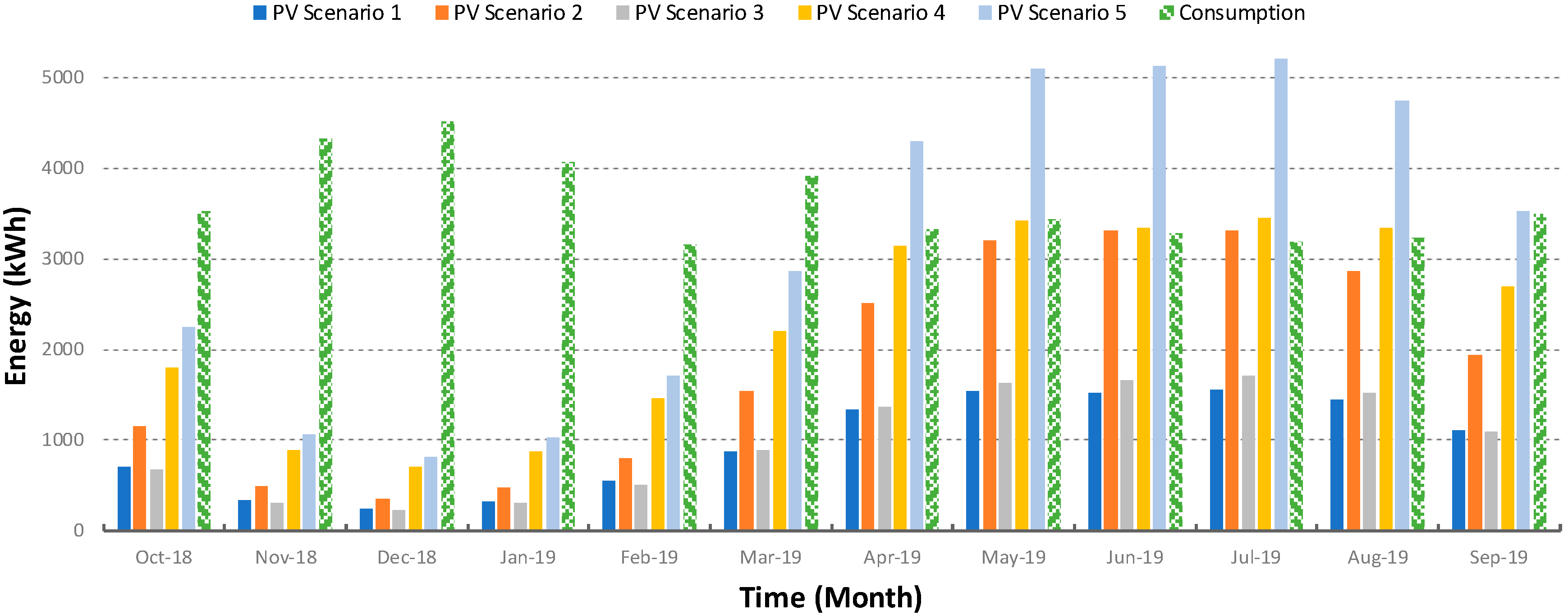
3.2. PV Scenarios

The study reported in this paper comprises five distinct scenarios used for the investigation of the effect of the PV configuration (Figure 8) on the self-consumption and self-sufficiency of the building. The first scenario corresponds to the rooftop PV system that maximizes the PV generation (per kW_p on installed capacity) on an annual basis. In this case, PV modules are installed considering the orientation and inclination with the maximum annual irradiation, i.e., a 30° slope facing South for the climate conditions of Prague. Photovoltaic modules are spaced properly for minimizing the self-shading, forming an array with 11.28 kW_p installed capacity (Figure 8). The second scenario corresponds to the rooftop PV system arrangement (shaded-free) with the maximum installed capacity. In this case, PV modules are placed following the shape of the roof in two orientations (SE-NW) considering a small tilt angle of 10°. The total installed capacity is increased by more than 50%, leading to a 24.48 kW_p PV array. The third scenario corresponds to a similar installation with a single orientation (SE) and an increased tilt angle of 25°. The PV capacity is slightly increased by 0.72 kW_p compared to Scenario 1 (lower shading effect). Peak generation is shifted from noon to morning hours, aiming to increase the self-consumption of the building (load matching). In the fourth and fifth scenarios, both roof and façade systems are taken into consideration based on the results obtained from the solar analysis. The former (Scenario 4) combines the rooftop PV—optimized for the maximum generation—and vertically attached on the SE and SW façades, as presented in (Figure 8). The capacity increases to 34.8 kW_p aiming to enhance peak generation during the winter period. In the latter, the PV façade system is similarly added to the second PV scenario, leading to the maximum PV capacity (48 kW_p). In this case, a broader PV generation curve is expected, maximizing the self-consumption as a direct consequence of multiple orientations and tilt angles (Scenario 5).

Afterwards, battery energy storage is introduced to provide a certain degree of energy flexibility. In this case, the introduced energy flexibility is used to improve the load matching and thus maximize the PV self-consumption and grid stability. Different BESS are considered in this study with storage capacity between 10 and 75 kWh. In the end, conclusions are drawn for the optimal sizing of the PV-BESS system based on the calculated metrics.

3.3. PV Modeling and Generation

The estimation of the outputs of the PV systems installed on the roof and façades was carried out using the one-diode five parameters model represented by Equation (1):

$$I=I_{ph}-I_o\left(e^{\left(\frac{V+R_{s}I}{n{V}_t}\right)}-1\right)-\left(\frac{V+R_{s}I}{R_{sh}}\right)$$

(1)

where I_ph is the photogenerated controlled current source, n is the diode ideality factor, and I_o is the reverse saturation current. Finally, a shunt resistance R_sh and a series resistance R_s represent the power losses.

The calibration of the PV model as well as the estimation of its unknown parameters was carried out by following the same procedure already published in [38]. The validation of the model was done based on real measured data from our PV plants consisting of polycrystalline PV panels [39]. The characteristics of the panel are listed in

Table 2. PV and battery energy storage system (BESS) main parameters.

BESS Technology	Li-Ion NMC	PV Technology	mc-Si
Efficiency	97%	Module area	1.58 m2
Energy	6.3 kWh	Efficiency	14.9 %
Nominal voltage	54.7 V	Tem. Coeff.	P: −0.44%/K, Voc: −0.3%/K, Isc: 0.04 %/K
Nominal capacity	116 Ah
Max. charge current	80 A	Pmp	245 W
Max. discharge current	300 A (3 sec.)	Voc	37.1 V
Self-discharge (cells)	4%/year	Isc	8.74 A
Discharge depth (DOD)	80%	Vmp	29.9 V
Full cycles	5000	Imp	8.19 A

. The calculation of the module temperature (T_m) for the PV system on the roof was done using the nominal operating cell temperature (NOCT) formula defined by Equation (2).

$$T_m=T_a+\frac{NOCT-20}{800}G$$

(2)

where T_a is the ambient measured temperature on the roof, and G is the on-plane irradiance falling on the PV module. In case of BIPV, the connection between the building envelope and PV array was realized by a two-sided temperature transfer using Type-567 from the Green Building TESS library [40]. Then, the module temperature of the PV panels installed on the façades (considering an open cavity) was used as an input in the following equation (Equation (3)) for the calculation of the BIPV efficiency.

$${\eta }_{BIPV}={\eta }_{BAPV}\left[1-{\gamma }_P\left(T_{BIPV}-T_{BAPV}\right)\right]$$

(3)

where γ_P is the temperature coefficient, η is the efficiency, and T the temperature of free-standing and BIPV module.

According to the definition of the PV scenarios, the system capacity ranges between 22 and 48 kW_p with an average annual simulated performance from 897 to 1023 kWh/kW_p for the rooftop PV systems and only 670 kWh/kW_p for the façade system, respectively (see

Table 3. Parameters of the designed PV scenarios.

PV System	Suitable Surface (%)	No PV Modules	Capacity (kWp)	Performance kWh/kWp
Roof_1	22	47	11.3	1023.5
Roof_2	47.6	102	24.5	897.2
Roof_3	23.3	50	12	990.4
Facade	19.6	98	23.5	670.2

). The renewable energy share that could be achieved ranges between 26.4% (Scenario 1) and 86.3% (Scenario 5), while the rest of the electricity demand should be provided by the grid.

A finer analysis of the matching issues is reported through the comparison between demand and generation presented in Figure 9. The blue line represents the typical load profile (hourly intervals), which approximately reflects the building’s occupancy (see Section 2). The rest correspond to the typical generation profiles of the PV systems and reflect the availability of the respective primary energy resource. The shape of the load curves remains similar all over the year with only minor monthly fluctuations. The main difference is observed in the peak loads, which range between 6 kW during the summer and 9 kW in winter period. From this hourly representation, it is easy to notice that the PV power rarely matches the peak demand for Scenarios 1 and 3. This happens only during the summer period, where Scenario 3 follows the morning peak representing a high level of self-consumption. By increasing the PV capacity (Scenario 2), a broader PV curve is observed. In summer, higher generation in conjunction with lower demand leads to a surplus of energy (from 09:00 to 15:00) and thus lower self-consumption. Conversely, during the winter time, the electricity demand is higher and the PV generation is significantly lower compared to the summertime (poor matching). The addition of the façade PV system increases significantly the PV generation and thus the load matching during the winter months.

Then, hourly load matching was calculated excluding the period of time without solar radiation. For Scenario 1, it was found to be 16% of the time, which was much lower compared to the monthly cover values (up to 49%). Similar values were found for Scenario 3 (17.3%), while a further increase is reported for Scenario 2. The best performance was obtained for Scenario 5, where the PV system can effectively match the building’s demand 50.8% of the time. The referred mismatch between electricity demand and PV generation is expected to be further reduced through the integration of the BESS discussed in the following subsection.

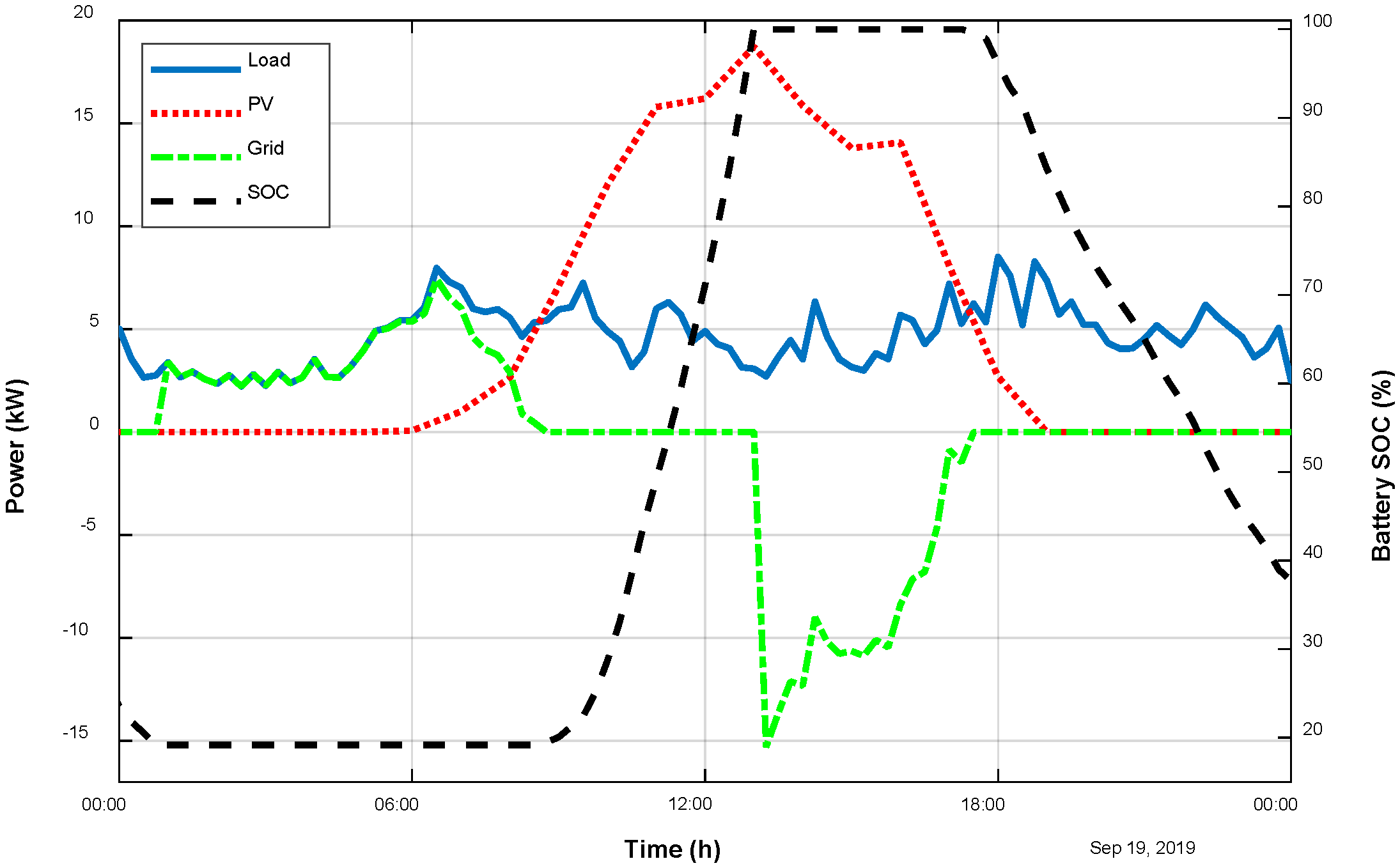
3.4. BESS Modeling and Control Strategy

The battery energy storage system (BESS) can mitigate the intermittency of the power generated from the PV system, store the surplus energy, and provide other ancillary services to the electricity grid. In this work, a lithium-ion (Li-Ion NMC) battery technology was considered in the simulations, as this type of batteries has been already modeled and validated in previous works [39,41]. The main parameters of a single battery module are listed in Table 2.

The dynamic behavior of the BESS has been simulated using the mathematical model described more in detail in [42]. The mathematical model of the battery allows the estimation of the instantaneous normalized value of the state of charge (SOC_n in [%]) at any the time (t) using Equation (4). The battery current (I_bat) can be positive or negative, depending on the discharging and charging modes, respectively. The voltage V₁ varies according to the charging and discharging modes, and its definition can be found in [42].

$$SO{C}_n\left(t\right)=SO{C}_i+\frac{1}{SO{C}_m}{{\displaystyle \int }}^{}\left(\frac{k{V}_1{I}_{bat}}{3600}-\frac{DSO{C}_n\left(t-\tau \right)SO{C}_m}{3600}\right)dt$$

(4)

The variables in Equation (4) are: SOC_i, which represents the initial battery state of charge in percentage [%]. SOC_m is the maximum battery state of charge in watt-hour [Wh]. The self-discharge and the charge/discharge efficiency are D and k, respectively. The variable τ represents the internal timestep used by the software in the simulation. This battery model was already validated in previous works published in [39,41], and it presented a good accuracy in the estimation of the SOC of the battery. Root mean square error (RMSE) values less than 5% were obtained when comparing simulations and real measured data [39,41].

The energy management control strategy could have a significant impact on the operation of the BESS with the PV system. There are various energy management control strategies that can ensure an effective operation of hybrid PV/BESS systems considering different aspects. These aspects can be related to the cost and economics of the system operation, respecting some constraints and rules related to the power injection to the grid, limitation of the use of the gird, peak shaving, etc. In this study, the load following control strategy (LFCS) is considered due to its simple implementation in real life as well as to its effectiveness in maximizing the self-consumption of the on-site generated power. A detailed description of this LFCS can be found in [41,43]. The LFCS follows some rules that are described below based on a one-day simulation of our hybrid system composed of PV/BESS and the grid shown in Figure 10.

The BESS can only be charged from the PV system, and it is never charged from the grid. When there is no PV energy and the BESS state of charge (SOC) is equal to SOC_min (from Figure 10, SOC_min = 20%), the load is supplied directly from the grid. Once the PV system starts generating power, the use of the grid is reduced accordingly in order to supply the load from the PV and grid simultaneously. When the PV power becomes higher than the load and the SOC of the battery is below its maximum limit, the load is supplied from the PV; meanwhile, the excess of energy will charge the BESS. When the SOC of the BESS reaches its maximum limit and still the PV power is higher than the load, in that case, the surplus power is injected to the grid, as it can be seen in Figure 10 at time between 13:00 and 18:00. At the end of the day, the BESS takes over the supply of the load when its SOC is higher than the SOC_min value and the PV power is lower than the demand (Load).

4. Discussion

The MATLAB^® environment was used for the implementation of the PV and BESS models, as well as the control strategy in order to simulate the electrical behavior of the building along the monitored campaign ranging from October 2018 to September 2019. The building performance has been simulated considering the five PV scenarios described in Section 3.2. Each PV scenario has been simulated with various BESS capacities ranging from zero (case without BESS) up to 75 kWh based on the load following control strategy (LFCS).

The results obtained from the simulations are given in terms of monthly values corresponding to energy consumption, PV energy generation, excess of energy sent to the grid, and the total energy taken from the grid. Detailed results can be found in Appendix A, where the five tables (

Table A1. Energy sent/taken to/from the grid considering various BESS capacities obtained for PV Scenario 1.

PV Scenario 1
	No BESS		BESS = 10 kWh		BESS = 20 kWh		BESS = 50 kWh		BESS = 75 kWh
	Excess (kWh)	Grid (kWh)	Excess (kWh)	Grid (kWh)	Excess (kWh)	Grid (kWh)	Excess (kWh)	Grid (kWh)	Excess (kWh)	Grid (kWh)
10/18	78.3	2904	28.6	2848.8	11.2	2827.3	0	2805	0	2797.4
11/18	1	3997.8	0	3993.3	0	3990.3	0	3981.2	0	3973.4
12/18	0.2	4267.2	0	4263.7	0	4260.8	0	4251.8	0	4243.2
01/19	2.2	3743.0	0	3737.5	0	3734.1	0	3724.8	0	3717.6
02/19	44.8	2647.6	3.8	2601.9	0	2594.5	0	2585	0	2577.3
03/19	70.2	3095.9	24.6	3045.0	7.4	3025.1	0	3006.1	0	1998.4
04/19	242.5	2236.4	95.0	2084.9	23.4	2002.6	0	1966.6	0	1958.9
05/19	238.9	2147.6	94.7	1998.6	38.6	1935.5	0	1881.6	0	1873.7
06/19	285.1	2040.8	133.9	1882.6	58.6	1802.4	0	1726.4	0	1718.7
07/19	317.2	1955.2	146.2	1780.4	58.6	1681.6	0	1606.6	0	1599.4
08/19	240.2	2033.3	78.8	1865.4	18.4	1795.9	0	1765.1	0	1758
09/19	124.9	2513.6	30.9	2413.7	4.5	2381.8	0	2367.2	0	2359.5

,

Table A2. Energy sent/taken to/from the grid considering various BESS capacities obtained for PV Scenario 2.

PV Scenario 2
	No BESS		BESS = 10 kWh		BESS = 20 kWh		BESS = 50 kWh		BESS = 75 kWh
	Excess (kWh)	Grid (kWh)	Excess (kWh)	Grid (kWh)	Excess (kWh)	Grid (kWh)	Excess (kWh)	Grid (kWh)	Excess (kWh)	Grid (kWh)
10/18	220.7	2602.1	101.8	2478.8	64.5	2432.7	9	2364.6	0	2346.1
11/18	5.6	3836.7	0	3827.3	0	3824.4	0	3815.1	0	3807.5
12/18	0	4168.2	0	4164.7	0	4161.9	0	4152.7	0	4144.3
01/19	4.9	3583.8	0	3575.2	0	3572.1	0	3562.9	0	3555.2
02/19	102.1	2455.4	24.9	2373.4	6.1	2348.8	0	2332.9	0	2325.1
03/19	284.5	2646.8	141.3	2500.8	81.9	2431.9	5.3	2338.1	0	2325.1
04/19	994.6	1824.1	764.4	1600.4	579.9	1408.2	207	992.9	74	843.5
05/19	1315	1553.6	1045.6	1287.3	846.1	1078.7	404.2	628.3	263.1	482.7
06/19	1468.6	1438.4	1209.6	1186.1	1026.6	992.4	679.8	633.9	552.2	516
07/19	1524.6	1405	1246.3	1138.3	1035.5	914.1	554.3	419.9	361.8	223.2
08/19	1190.5	1568.6	933.3	1317.2	723.3	1096.3	270.5	611.9	135.1	468
09/19	552.3	2100.6	357.2	1902	233.7	1774.3	37.6	1548.3	1	1500.1

,

Table A3. Energy sent/taken to/from the grid considering various BESS capacities obtained for PV Scenario 3.

PV Scenario 3
	No BESS		BESS = 10 kWh		BESS = 20 kWh		BESS = 50 kWh		BESS = 75 kWh
	Excess (kWh)	Grid (kWh)	Excess (kWh)	Grid (kWh)	Excess (kWh)	Grid (kWh)	Excess (kWh)	Grid (kWh)	Excess (kWh)	Grid (kWh)
10/18	63.1	2924.6	24.8	2881.5	8.3	2861.3	0	2842.7	0	2834.9
11/18	0	4027.7	0	4024.3	0	4021.4	0	4012.1	0	4004.5
12/18	0.2	4282.9	0	4279.4	0	4276.5	0	4267.5	0	4258.9
01/19	0.6	3757.6	0	3753.2	0	3750.2	0	3741.3	0	3733.3
02/19	31.5	2675.4	0	2639.3	0	2636.1	0	2626.4	0	2619.2
03/19	62.5	3080.2	15.8	3029.6	4	3012.4	0	2998.7	0	2991
04/19	252.1	2208.4	106.8	2059.8	33.9	1976.1	0	1928.4	0	1920.8
05/19	283.6	2095.4	131.5	1939.3	58.1	1857.1	0	1782.9	0	1775.2
06/19	355.6	1982.3	187	1811.5	95.7	1709.6	1.4	1595.4	0	1586
07/19	385.8	1877.1	200.8	1689.3	87.6	1564.9	0	1455.8	0	1448.9
08/19	285.3	1996.2	110.3	1820	27.7	1722.3	0	1681.7	0	1674
09/19	105.5	2515.2	24.8	2428.8	5.9	2403.8	0	2388.6	0	2381.2

,

Table A4. Energy sent/taken to/from the grid considering various BESS capacities obtained for PV Scenario 4.

PV Scenario 4
	No BESS		BESS = 10 kWh		BESS = 20 kWh		BESS = 50 kWh		BESS = 75 kWh
	Excess (kWh)	Grid (kWh)	Excess (kWh)	Grid (kWh)	Excess (kWh)	Grid (kWh)	Excess (kWh)	Grid (kWh)	Excess (kWh)	Grid (kWh)
10/18	717.1	2451.8	508.6	2252.4	386.8	2111.7	193.3	1895.1	117.2	1805.1
11/18	185.3	3622.9	81.7	3516.8	43.1	3471.9	2.5	3415.4	0	3405
12/18	121.4	3923.5	37.3	3838.2	3.6	3796.7	0	3780.8	0	3772.9
01/19	167.5	3354.7	85.7	3268.9	52.4	3233.1	9.9	3174.9	0	3155.8
02/19	592.9	2280.9	426.5	2118.5	323.4	2005.7	148.1	1804.4	42.3	1686.9
03/19	775.9	2485.4	574	2279.2	433.5	2133.7	197.8	1884	120.9	1796.4
04/19	1558.8	1754	1324.9	1531.8	1134.6	1330.2	654.7	816.7	480.3	628.5
05/19	1511.7	1532.4	1248.2	1276.5	1038.7	1056.8	587.3	592.3	426.4	428.1
06/19	1498.1	1441.5	1243.6	1188.4	1057.6	1000.2	704.1	644.8	587.7	524.4
07/19	1656.8	1405.1	1380	1137.6	1171.1	917.7	685.3	418.7	489.3	212.7
08/19	1623.5	1528.5	1364.4	1274.8	1154	1057.6	654.5	533.1	478.4	362.4
09/19	1194.7	1997.6	985.7	1791.3	824.9	1624	473.6	1263.2	296.4	1086.2

and

Table A5. Energy sent/taken to/from the grid considering various BESS capacities obtained for PV Scenario 5.

PV Scenario 5
	No BESS		BESS = 10 kWh		BESS = 20 kWh		BESS = 50 kWh		BESS = 75 kWh
	Excess (kWh)	Grid (kWh)	Excess (kWh)	Grid (kWh)	Excess (kWh)	Grid (kWh)	Excess (kWh)	Grid (kWh)	Excess (kWh)	Grid (kWh)
10/18	1011.2	2301.5	782.3	2079.1	619.2	1907.1	295.1	1549.1	199.4	1438
11/18	225.7	3497.5	110.1	3376.4	62.5	3323.8	5.6	3251.3	0	3237
12/18	137.6	3840.5	46.6	3745.1	6.3	3701.3	0	3679.8	0	3673.2
01/19	205.5	3230.8	98.2	3121.5	67	3084.6	12.8	3014.9	0	2992
02/19	737.1	2175.6	546.9	1998.3	422.6	1854.8	185.8	1595.5	74.4	1467.6
03/19	1248.8	2295	997.1	2053.4	816.4	1863.8	431.5	1452	267.8	1290.8
04/19	2547	1577.9	2295.8	1338.2	2094.1	1133.9	1530.1	546	1347.7	367.9
05/19	2953	1303.5	2651.3	1021	2416.1	775.7	1818.3	171.8	1687.4	38.5
06/19	3039.5	1197.1	2761.5	928.3	2539.4	702.3	2068.8	243.2	1947.4	121
07/19	3206.3	1197	2913.2	915.4	2675.7	670.8	2134.2	123.6	2018.7	26.1
08/19	2853.7	1343.7	2563.1	1070.2	2344.3	838.8	1751.4	227.1	1596.1	78
09/19	1870.1	1832.4	1628	1599.9	1452.3	1416	980.1	924.4	749.1	701.9

) illustrate the monthly energy sent/taken to/from the utility grid according to each PV scenario. The rest of the variables related to the monthly PV generations and the monthly load consumption are given in Figure 11.

Figure 11 evaluates the monthly energy matching between consumption and generation for each PV scenario. It can be seen that the consumption is higher during winter months compared to summer months. The highest PV energy generation is related to Scenario 5, and it is observed during the period April–August, where the PV generation is almost 40% higher compared to the other scenarios. However, during winter months, when the PV generation is the most needed, Scenario 5 generates almost the same amount of energy as Scenario 4. So, in terms of effective usage of local generated electricity, Scenario 4 is preferable to Scenario 5. Scenarios 1 and 3 provide the same results, and this is due to the orientation of the two houses. Regarding Scenario 2, where the PV panels are installed only on the roof considering a low tilt angle, it can be seen that this scenario provides better results compared to Scenarios 1 and 3. PV generation during winter months is increasing slightly for the increased PV capacity of Scenario 2 and becomes more than two times higher with the addition of the façade system (Scenarios 4, 5). This increase of the PV production in winter months demonstrates the benefits of combining rooftop PVs with façades PVs (Scenarios 4 and 5).

Two load matching indicators, Self-consumption (S_c) and Self-sufficiency (S_s), have been used for the evaluation of each PV and BESS combination. The S_c represents the amount of the generated PV energy that is consumed locally or sent to the BESS. Meanwhile, the S_s indicates the percentage of the building ability in being autonomous. The S_c and S_s are defined by the following equations.

$$S_c(\%)=100\left(1-\frac{E_{to\_G}}{E_{PV}}\right)$$

(5)

$$S_s(\%)=100\left(1-\frac{E_G}{E_L}\right)$$

(6)

where E_{to_G} is the excess of energy sent to the utility grid, E_PV is the accumulative energy generated from the PV array, E_G is the energy taken from the utility grid, and E_L represents the energy consumed by the load.

Figure 12 summarizes the average annual rates of the S_c and S_s calculated from the monthly values related to PV energy generation according to the different PV scenarios, various BESS capacities, as well as the grid and excess data listed in Table A1, Table A2, Table A3, Table A4 and Table A5. The results show that for the considered PV sizes and BESS capacities, the S_c and S_s of the building could vary from 55% to 100% and from 24% up to 68%, respectively. It can be seen that the S_c is lower than 60% when there is no BESS and the PV size is higher than 40 kW_p. In order to achieve the maximum value of the self-consumption (S_c > 99%), the PV size should not exceed 11 kW_p and the BESS capacity should be higher than 55 kWh. This solution (achieving a S_c > 99%) is not suitable, as it provides S_s values lower than 30% and it is also uneconomical, as the BESS price is still expensive. Regarding the S_s indicator, the highest value is obtained for the PV sizes and BESS capacities above 43 kW_p and 56 kWh, respectively. The case related to the highest S_s (above 65%) corresponds to the most expensive scenario, as it requires a big PV size and large BESS capacity. A good compromise between the two indicators in terms of excess of energy optimization can be represented by values around 75% for the S_c and 50% for the S_s.

The value of the two indicators can highly be affected by the employed energy dispatch control strategy. From previous work published in [41], it was concluded that the LFCS gives the highest values of the self-sufficiency indicator, and this is mainly related to the fact that the BESS is never charged from the utility grid.

The obtained results shown in Figure 12 provide a global idea about the variation of the two load matching indicators (S_c and S_s) based on the LFCS considering various PV sizes and BESS capacities. The graphs can be used for the selection of the range of PV system size and the BESS capacities, which provide S_c above a certain value. As for example, in the case of the Czech Republic, in order to get subsidies from the New Green Savings programme, which is financed from the proceeds of the sale of the so-called EUA (European Union Allowance) and EUAA (European Union Aviation Allowance) emission allowances, the annual self-consumption of the local generated PV energy should be above 70% [44]. Moreover, the two graphs can be used for the evaluation of the performance of buildings with similar characteristics such as the one considered in this work.

The consideration of façades for the integration of PV systems is one of the key parameters for increasing the load matching indicators in residential buildings. In building with flat roofs, lower tilt angles up to 10° with E and W orientations will provide a wider PV generation profile and limit the peak power around noon, leading to significant savings in the selection of the appropriate inverter size. Other parameters that should be taken into account for the reproduction of the obtained results concerning the S_c and S_s are related to the building typology (administrative, residential, etc.), building configuration (installation size, available area), the geographical location (climate, state policy), and consumption patterns.

Finally, the choice of the optimum PV size and the adequate BESS capacity will mainly depend on the economical aspect. In this study, we have presented some technical solutions showing the effects of various PV systems and BESS capacities on the performance of a real monitored building. The optimal solution has to be extracted considering the economical aspect and a sophisticated control strategy—including PV forecasting, grid pricing policies, and other ancillary services related to the utility grid—which will be unique for a specific building (system).

5. Conclusions

The present paper investigated the electrical performance of two bloc-of-flats buildings in Prague, based on real monitored data collected from October 2018 to September 2019. The analysis of the measured data revealed some general trends in the residential load profiles. Generally, the shape of the monthly load curves remains almost similar all over the year with only minor fluctuations. Main differences were observed in the peak loads between the winter and summer periods. The analysis of the effect of photovoltaic (PV) and battery energy storage systems (BESS) on the overlap between electricity generation and demand was done in a MATLAB environment using validated PV and BESS models.

Five PV scenarios were defined considering various configurations including rooftop and façade PV systems. The PV scenarios were evaluated according to their characteristics for matching the load considering their sizes ranging between 11 and 48 kW_p. The results indicated that there is a seasonal variation between the match of load and local PV generation in Prague. In this context, optimized array tilt and orientation angles can effectively contribute to a better adjustment. The load matching indicators are further improved by including the battery energy storage. The five PV scenarios were simulated based on the load following control strategy considering different BESS capacities in order to show their effects on the self-consumption (S_c) and the self-sufficiency (S_s) indicators. For the considered PV sizes and BESS capacities, the Sc and Ss of the building could vary from 55% to 100% and from 24% to 68%, respectively.

Targeting the maximal S_c value is uneconomical, as it requires small PV size and large BESS capacity; in addition, it leads to lower Ss values. A PV system of 35 kWp combined with a BESS of 20 kWh capacity was proven to be a very promising solution to address the load-matching issue of such residential buildings, resulting in S_c and S_s values above 75% and 50%, respectively. Parameters such as solar availability, household construction, and operation are Czech-specific, and results are valid for hybrid energy systems with the same control strategy. Specific findings and recommendations are not universal and might differ when other climates and/or jurisdictions are concerned. On the other hand, the elaborated methods and approaches could be replicable to any location worldwide.

Finally, the choice of the optimum PV-BESS sizes requires considering the economical aspect as well as the development of a sophisticated energy management control strategy—including PV forecasting, grid pricing policies, and other ancillary services related to the utility grid. Future study will be carried out to evaluate the impact of different control strategies. Furthermore, the feasibility of the proposed solution will be studied in depth—considering the actual costs, supporting programs and policies—in order to generalize the deployment of PV-BESS systems in residential buildings.

References

- UNEP (United Nations Environment Programme). Building Design and Construction: Forging Resource Efficiency and Sustainable Development; UNEP: Nairobi, Kenya, 2012. [Google Scholar]
- Directive 2010/31/EU of the European Parliament and of the Council of 19 May 2010 on the energy performance of buildings (recast). Off. J. Eur. Communities 2010, L153/13.
- IEA-PVPS Trends 2018 in photovoltaic applications. Survey Report of Selected IEA Countries between 1992 and 2017. Available online: http://www.iea-pvps.org (accessed on 20 April 2020).
- Luthander, R.; Widén, J.; Nilsson, D.; Palm, J. Photovoltaic self-consumption in buildings: A review. Appl. Energy 2015, 142, 80–94. [Google Scholar] [CrossRef] [Green Version]
- Gjorgievski, V.Z.; Chatzigeorgiou, N.G.; Venizelou, V.; Christoforidis, G.C.; Georghiou, G.E.; Papagiannis, G.K. Evaluation of Load Matching Indicators in Residential PV Systems-the Case of Cyprus. Energies 2020, 13, 1934. [Google Scholar] [CrossRef] [Green Version]
- Alrawi, O.; Bayram, I.S.; Al-Ghamdi, S.G.; Koc, M. High-Resolution Household Load Profiling and Evaluation of Rooftop PV Systems in Selected Houses in Qatar. Energies 2019, 12, 3876. [Google Scholar] [CrossRef] [Green Version]
- Aelenei, D.; Lopes, R.A.; Aelenei, L.; Gonçalves, H. Investigating the potential for energy flexibility in an office building with a vertical BIPV and a PV roof system. Renew. Energy 2019, 137, 189–197. [Google Scholar] [CrossRef] [Green Version]
- Brito, M.C.; Freitas, S.; Guimarães, S.; Catita, C.; Redweik, P. The importance of facades for the solar PV potential of a Mediterranean city using LiDAR data. Renew. Energy 2017, 111 (Suppl. C), 85–94. [Google Scholar] [CrossRef]
- Freitas, S.; Reinhart, C.; Brito, M.C. Minimizing storage needs for large scale photovoltaics in the urban environment. Sol. Energy 2018, 159, 375–389. [Google Scholar] [CrossRef]
- Mubarak, R.; Weide Luiz, E.; Seckmeyer, G. Why PV Modules Should Preferably No Longer Be Oriented to the South in the Near Future. Energies 2019, 12, 4528. [Google Scholar] [CrossRef] [Green Version]
- Skandalos, N.; Tywoniak, J. Influence of PV facade configuration on the energy demand and visual comfort in office buildings. J. Phys. Conf. Ser. 2019, 1343, 012094. [Google Scholar] [CrossRef]
- Nair, N.-K.C.; Garimella, N. Battery energy storage systems: Assessment for small-scale renewable energy integration. Energy Build. 2010, 42, 2124–2130. [Google Scholar] [CrossRef]
- Barbour, E.; Parra, D.; Awwad, Z.; González, M.C. Community energy storage: A smart choice for the smart grid? Appl. Energy 2018, 212, 489–497. [Google Scholar] [CrossRef]
- Angenendt, G.; Zurmühlen, S.; Axelsen, H.; Sauer, D.U. Comparison of different operation strategies for PV battery home storage systems including forecast-based operation strategies. Appl. Energy 2018, 229, 884–899. [Google Scholar] [CrossRef]
- Parra, D.; Patel, M.K. The nature of combining energy storage applications for residential battery technology. Appl. Energy 2019, 239, 1343–1355. [Google Scholar] [CrossRef]
- Vieira, F.M.; Moura, P.S.; de Almeida, A.T. Energy storage system for self-consumption of photovoltaic energy in residential zero energy buildings. Renew. Energy 2017, 103, 308–320. [Google Scholar] [CrossRef]
- Chatzivasileiadi, A.; Ampatzi, E.; Knight, I. Characteristics of electrical energy storage technologies and their applications in buildings. Renew. Sustain. Energy Rev. 2013, 25, 814–830. [Google Scholar] [CrossRef]
- Widén, J.; Wäckelgård, E.; Lund, P.D. Options for improving the load matching capability of distributed photovoltaics: Methodology and application to high-latitude data. Sol. Energy 2009, 83, 1953–1966. [Google Scholar] [CrossRef]
- Nyholm, E.; Goop, J.; Odenberger, M.; Johnsson, F. Solar photovoltaic-battery systems in Swedish households—Self-consumption and self-sufficiency. Appl. Energy 2016, 183, 148–159. [Google Scholar] [CrossRef] [Green Version]
- Pilz, M.; Ellabban, O.; Al-Fagih, L. On Optimal Battery Sizing for Households Participating in Demand-Side Management Schemes. Energies 2019, 12, 3419. [Google Scholar] [CrossRef] [Green Version]
- Kotarela, F.; Kyritsis, A.; Papanikolaou, N. On the Implementation of the Nearly Zero Energy Building Concept for Jointly Acting Renewables Self-Consumers in Mediterranean Climate Conditions. Energies 2020, 13, 1032. [Google Scholar] [CrossRef] [Green Version]
- Bertsch, V.; Geldermann, J.; Lühn, T. What drives the profitability of household PV investments, self-consumption and self-sufficiency? Appl. Energy 2017, 204, 1–15. [Google Scholar] [CrossRef] [Green Version]
- Litjens, G.B.M.A.; Worrell, E.; van Sark, W.G.J.H.M. Economic benefits of combining self-consumption enhancement with frequency restoration reserves provision by photovoltaic-battery systems. Appl. Energy 2018, 223, 172–187. [Google Scholar] [CrossRef]
- Sani Hassan, A.; Cipcigan, L.; Jenkins, N. Optimal battery storage operation for PV systems with tariff incentives. Appl. Energy 2017, 203, 422–441. [Google Scholar] [CrossRef]
- Barbour, E.; González, M.C. Projecting battery adoption in the prosumer era. Appl. Energy 2018, 215, 356–370. [Google Scholar] [CrossRef] [Green Version]
- Cucchiella, F.; D’Adamo, I.; Gastaldi, M. The Economic Feasibility of Residential Energy Storage Combined with PV Panels: The Role of Subsidies in Italy. Energies 2017, 10, 1434. [Google Scholar] [CrossRef]
- Kosmadakis, I.E.; Elmasides, C.; Eleftheriou, D.; Tsagarakis, K.P. A Techno-Economic Analysis of a PV-Battery System in Greece. Energies 2019, 12, 1357. [Google Scholar] [CrossRef] [Green Version]
- Goebel, C.; Cheng, V.; Jacobsen, H.-A. Profitability of Residential Battery Energy Storage Combined with Solar Photovoltaics. Energies 2017, 10, 976. [Google Scholar] [CrossRef] [Green Version]
- Parra, D.; Norman, S.A.; Walker, G.S.; Gillott, M. Optimum community energy storage for renewable energy and demand load management. Appl. Energy 2017, 200, 358–369. [Google Scholar] [CrossRef]
- Pena-Bello, A.; Burer, M.; Patel, M.K.; Parra, D. Optimizing PV and grid charging in combined applications to improve the profitability of residential batteries. J. Energy Storage 2017, 13, 58–72. [Google Scholar] [CrossRef]
- Denholm, P.; Nunemaker, J.; Gagnon, P.; Cole, W. The potential for battery energy storage to provide peaking capacity in the United States. Renew. Energy 2020, 151, 1269–1277. [Google Scholar] [CrossRef]
- Solano, J.C.; Olivieri, L.; Caamaño-Martín, E. Assessing the potential of PV hybrid systems to cover HVAC loads in a grid-connected residential building through intelligent control. Appl. Energy 2017, 206, 249–266. [Google Scholar] [CrossRef]
- Liu, J.; Chen, X.; Yang, H.; Li, Y. Energy storage and management system design optimization for a photovoltaic integrated low-energy building. Energy 2020, 190, 116424. [Google Scholar] [CrossRef]
- Spasic, D. Gismo Plugin. Available online: https://github.com/stgeorges/gismo/ (accessed on 15 April 2020).
- SolemmaLLC, 2019. DIVA Version 4. Available online: http://www.solemma.com/ (accessed on 15 April 2020).
- Ward, G.J. The RADIANCE lighting simulation and rendering system. In Proceedings of the 21st Annual Conference on Computer Graphics and Interactive Techniques; Association for Computing Machinery: New York, NY, USA, 1994; pp. 459–472. [Google Scholar]
- Daysim Software. 2013. Version 4.0. Available online: http://daysim.ning.com/ (accessed on 15 April 2020).
- Kichou, S.; Silvestre, S.; Guglielminotti, L.; Mora-López, L.; Muñoz-Cerón, E. Comparison of two PV array models for the simulation of PV systems using five different algorithms for the parameters identification. Renew. Energy 2016, 99, 270–279. [Google Scholar] [CrossRef]
- Kichou, S.; Skandalos, N.; Wolf, P. Energy performance enhancement of a research centre based on solar potential analysis and energy management. Energy 2019, 183, 1195–1210. [Google Scholar] [CrossRef]
- Bradley, T. TYPE 567: Glazed building integrated photovoltaic system. In TESS Libraries version 2.0 General Descriptions; Thermal Energy System Specialists (TESS): Madison, WI, USA, 2004. [Google Scholar]
- Skandalos, N.; Kichou, S.; Wolf, P. Energy sufficiency of an administrative building based on real data from one year of operation. In Proceedings of the 2018 Smart City Symposium Prague (SCSP), Prague, Czech Republic, 24–25 May 2018; pp. 1–8. [Google Scholar]
- Castañer, L.; Silvestre, S. Modelling Photovoltaic Systems Using PSpice®; John Wiley & Sons, Ltd: Hoboken, NJ, USA, 2002. [Google Scholar]
- Ameen, A.M.; Pasupuleti, J.; Khatib, T. Simplified performance models of photovoltaic/diesel generator/battery system considering typical control strategies. Energy Convers. Manag. 2015, 99, 313–325. [Google Scholar] [CrossRef]
- State Environmental Fund of the Czech Republic, New Green Savings Programme. Available online: https://www.sfzp.cz/en/ (accessed on 15 April 2020).