Location and Sizing of Battery Energy Storage Units in Low Voltage Distribution Networks

Abstract

Proper planning of the installation of Battery Energy Storage Systems (BESSs) in distribution networks is needed to maximize the overall technical and economic benefits. The limited lifetime and relatively high cost of BESSs require appropriate decisions on their installation and deployment, in order to make the best investment. This paper proposes a comprehensive method to fully support the BESS location and sizing in a low-voltage (LV) network, taking into account the characteristics of the local generation and demand connected at the network nodes, and the time-variable generation and demand patterns. The proposed procedure aims to improve the overall network conditions, by considering both technical and economic aspects. An original approach is presented to consider both the planning and scheduling of BESSs in an LV system. This approach combines the properties of metaheuristics for BESS sizing and placement with a greedy algorithm to find viable BESS scheduling in a relatively short time considering a specified time horizon, and the application of decision theory concepts to obtain the final solution. The decision theory considers various scenarios with variable energy prices, the diffusion of local renewable generation, evolution of the local demand with the integration of electric vehicles, and a number of planning alternatives selected as the solutions with top-ranked objective functions of the operational schedules in the given scenarios. The proposed approach can be applied to energy communities where the local system operator only manages the portion of the electrical grid of the community and is responsible for providing secure and affordable electricity to its consumers.

1. Introduction

The progress of technologies concerning different types of batteries and their control systems, together with the evolution of a regulatory framework in which energy storage is considered more explicitly, are making Battery Energy Storage Systems (BESSs) progressively more cost-effective for energy system applications. A BESS is specified by its power rating and energy capacity. Both of these specifications impact the BESS investment cost and need to be defined separately [1]. Typical BESS applications for power and energy systems include improvement of the quality of service, assistance with primary and secondary frequency control to enhance network stability, the smoothing of power fluctuations in the generation profiles for better integration of Renewable Energy Sources (RES), and the promotion of higher users’ participation in demand management through time-shifting of the energy usage [2]. Most BESS applications in electrical networks refer to times of 1–2 h and to BESS sizes smaller than 50 kW. However, the number of applications for longer times (e.g., 2–5 h) and sizes up to 500 kW is already significant, and applications for bigger sizes (also in the range 1–10 MW) are increasing.

In the transmission system, the positive impacts of BESSs for providing a fast response to frequency deviations [3], mitigating under-frequency transients [4], and being exploited for energy arbitrage [5] have been observed. The integration of BESSs with appropriate control strategies has been shown to be able to improve the frequency stability [6]. At the distribution system level, a BESS is mainly used for enhancing the grid integration of RES by mitigating the effects of the uncertainty on load and distributed generation [7,8], improving the distribution system reliability by avoiding operations close to the line thermal limits and thus more exposed to the risk of protection trips [9], enhancing the quality of the supply with relatively high-power and low-energy solutions [10], reducing the need for grid expansion, shaving the power demand peaks through load shifting or load leveling [9], optimizing the energy transaction costs [11], and integrating BESSs with the demand response in microgrid applications [12]. In [13], a distinction is made between a centralized BESS (that participates in reducing the demand deviation, avoiding the reverse power flow and correcting the power factor), and a distributed BESS (that aims at annual energy loss reduction, reduction of the demand deviation, and improvement of the voltage profile).

A key challenge is to determine the power rating, energy capacity, and location of BESSs in the distribution network. A number of contributions have been published on the siting and sizing of BESSs. Different objectives, such as peak shaving, voltage regulation, and reduction of the energy not supplied, are combined in [14] in an optimal power flow-based approach. In [15], reliability improvement, together with peak shaving, is considered as an objective. The review [16] presents a categorization of the methods used to determine the BESS siting and sizing, in which four main groups are identified (analytical methods, exhaustive search, mathematical programming, and heuristic methods). Decision-making tools are also applied. For example, in [17], the optimal BESS sizing and siting is identified in a microgrid with RES taking into account demand and generation uncertainty by using decision theory criteria. In [18], hybrid energy storage systems, including BESSs, are addressed, by determining the energy storage capacity in distribution systems through an assessment of the risk tolerance of the investors. The results of BESS installations in terms of providing different services at different voltage levels are reported in [19].

A specific aspect generally not highlighted in the reviews on BESS siting and sizing is the distinction between applications for Medium Voltage (MV) and Low Voltage (LV) systems. The literature contributions mainly refer to Medium Voltage (MV) distribution systems. However, the formulation of a planning problem referring to the installation of BESSs in LV systems has various differences with respect to what happens in MV systems. First of all, in MV systems, the study can be conducted by assigning growth in the local generation and demand aggregated at the MV node level. In this case, it is possible to mix up the contributions from different energy sources at the LV level, without looking at the details of the individual sources. Additionally, the uncertainty that characterizes the local generation is seen with respect to the aggregation of the generations, typically taking into account possible correlations between the generation patterns due to external variables (e.g., solar irradiance and temperature for photovoltaic systems). Then, it is possible to exploit the smoothing effect due to the aggregation of a number of individual demands, define typical patterns for the aggregated demand, and associate these typical patterns to predefined evolutions in time.

Conversely, for an LV system, the level of aggregation of demand and local generation is much lower, and many more critical aspects appear. In particular, the local characteristics of the generation and demand at each LV node have to be considered individually. The uncertainties of local generation and demand increase as the smoothing effect of the aggregations is reduced. The setting up of scenarios of development of the local generation cannot proceed with a generic aggregated effect at each LV node, but has to take into account where there are different types of local generation and what reasonable increment can be established for that type of generation. Some relevant differences between MV and LV systems are summarized in

Table 1. Summary of relevant differences between Medium Voltage (MV) and Low Voltage (LV) systems.

Characteristics	MV Grid	LV Grid	Consequences
Structure	Weakly meshed	Radial	LV grid cannot be reconfigured, thus the proper network operation has to be guaranteed thanks to the devices connected to the grid
Load	Balanced	Unbalanced	In the LV grid, it is advisable to apply three-phase load flow
Branch	R≈X	R>>X	In the LV grid, the voltage drop is strictly correlated to the active power, and voltage control can thus be effectively conducted by modifying the net nodal active power
Load profile	Aggregate	Not aggregate	LV grid represents the last mile of the grid and supplies the customer. A more detailed representation of loads and generation profiles is then necessary and the aggregation impact is less evident than in MV grids

.

To achieve the best BESS performance and to maximize the overall benefits, proper planning is necessary. For instance, in [20], several configurations of BESSs are compared and the overall network impact is evaluated and compared for different placements of BESSs in the network. In the relevant literature, there are some contributions related to the optimal planning (sizing and placement) of energy storage systems in LV distribution networks. The method applied in [21] aims to optimally configure the energy storage systems to alleviate over- and under-voltage problems. The problem of the optimal location is solved by a heuristic method based on voltage sensitivity analysis. Uncertainties due to stochastic generation and demand are also considered in the optimal sizing and the worst-case approach is applied to select the sizes.

Some contributions refer to LV distribution networks characterized by a high penetration of photovoltaic generation, and consider the possibility of alleviating the negative impacts by the installation of storage systems. In [22], a heuristic method is applied to determine the optimal location and sizing of storage systems and the objective to be minimized is a cost function accounting for the cost of storage systems and the cost due to voltage deviations. The optimal planning of BESSs proposed in [23] aims at maximizing an objective function that includes both benefits and costs (i.e., energy arbitrage, environmental emission, energy losses, transmission access fee, capital, and maintenance costs of a BESS). Daily charge/discharge of the storage systems is also determined considering a proper model of the BESS operation. In [24], the authors propose a procedure for the optimal placement and sizing of distributed energy storage systems in low voltage distribution systems aimed at maximizing the utilization of photovoltaic plants and minimizing the battery degradation. The multi-objective optimization problem proposed by [25] is focused, from one side, on the minimization of energy losses and, from the other side, on the minimization of costs associated with distributed generators and energy storage systems. A distribution system with a high penetration of photovoltaics generators is considered in [26]. A heuristic procedure for reducing the search space for the location of storage systems in a low voltage microgrid is proposed in [27], where analytical considerations on the voltage sensitivity, voltage unbalances, and line loading drive are included in the selection of candidate locations.

This paper proposes an overall procedure to address the BESS location and sizing in an LV network, taking into account the characteristics of the local generation and demand connected at the LV nodes and the time-variable generation and demand patterns. The proposed procedure aims to improve the overall network conditions by considering both technical and economic aspects. This condition aims to represent the conditions that could be found in the case of energy communities where the local system operator only manages the electrical grid of the community and is responsible for guaranteeing secure and affordable electricity for its consumers.

An original algorithm is presented to consider both the planning and scheduling of BESSs in an LV system. This algorithm combines the properties of metaheuristics (to explore the solution space as much as possible), and a greedy algorithm able to find viable BESS scheduling in a relatively short period of time, considering a specified time horizon. The final solution is obtained by using a multi-criteria decision making (MCDM) approach based on the application of decision theory concepts [28] to a number of selected planning alternatives evaluated for different weighted scenarios. Decision theory is an appropriate tool for dealing with cases in which the uncertainty on possible future situations is very large and is handled through scenario analysis.

The next sections of this paper are organized as follows. Section 2 describes the details of the methodology used to address the planning problem. Section 3 presents the application to an LV distribution system and discusses the results. The last section contains the concluding remarks.

2. Description of the Methodology

The BESS location and sizing is analysed as a planning problem seen from the point of view of the electricity manager of an energy community, which is responsible for guaranteeing secure and affordable electricity for its customers at a minimum cost, as well as for both the infrastructure and quality of the service.

2.1. Data Resolution and Reference Period

The data used are assumed to have a constant time resolution Δt. A reference period of duration T_ref is assumed, in which the operation of the LV distribution system is analysed in detail by considering the generation and demand patterns and a specific model for BESS scheduling. The planning problem is set up for a time horizon multiple of T_ref, namely, with an overall duration of T_H = N_H × T_ref, where N_H > 1 is an integer number. It is assumed that the BESSs that will be chosen by the proposed procedure will be installed at the beginning of the time period of analysis. The planning time horizon chosen is longer than the lifetime of the BESS, in order to include the replacement of the BESS during the planning period.

2.2. Definition of the Scenarios

The electricity prices, diffusion of the local generation, and diffusion of electric vehicles have been assumed to be uncertain data inputs that affect the solution of the planning problem. Several methods can be applied to handle uncertain variables; in this proposal, several scenarios will be identified to represent different instances.

Starting from the results determined for the reference period, a number of scenarios are constructed to represent possible paths of evolution of selected quantities that affect the LV network operation. The scenarios are defined by taking into account the long-term changes in time that may appear in the following quantities:

(a)

Electricity prices: the consumers or prosumers connected to the LV system are considered as price takers, namely, they do not participate in the definition of energy prices in the wholesale electricity market. M_P trends of variation of the electricity prices are established by the user by considering the final increase (or decrease) of the electricity price at the end of the planning time horizon;

(b)

Diffusion of the local generation: the distributed generation (DG) connected to the LV network can change at selected locations in different ways. For LV systems, it is likely that more prosumers will install their local generation systems at locations where there is no local production. From the point of view of the scenario definition, M_DG trends of variation of the local generation are considered, and each one is defined by assuming a rate of increase of the energy production from local generation (not of the power installed);

(c)

Diffusion of electric vehicles: in the present situation, the diffusion of EVs is still relatively limited in many jurisdictions. The number of EVs will increase in the future, and different hypotheses about their number can be represented by M_EV trends.

Under the hypotheses provided for the scenarios, the number of scenarios considered is equal to M = M_P × M_DG × M_EV.

The scenarios obtained are applied to calculate the objective function for the planning problem (Section 2.4), and are weighted in order to be used in the decision-based approach illustrated in Section 2.6.

2.3. Definition of the Sizing Alternatives

Due to the particular use of the BESS, which includes load leveling, the indication of [29] to use the energy to power ratio equal to 2 is followed. In this way, data are described in terms of their energy capacity, and the power rating is then directly linked to the energy capacity through the energy to power ratio.

In the distribution network, there are K nodes, but it is assumed that a user-defined number K_BESS < K of nodes is taken into account for possible BESS location. A maximum value for the BESS energy capacity C_k,max is assigned to each node k = 1,…, K_BESS, depending on the characteristics of the node. The final BESS energy capacity to be assigned to each node will be determined by the proposed approach in the range from zero to C_k,max at the nodes k = 1,…, K_BESS. To avoid the use of continuous variables, this range is partitioned into a given number Λ of BESS energy capacity levels. Without loss of generality, the number Λ is chosen as a constant for all the nodes, that is, it is independent of k. In this way, the total number of alternative combinations of BESS sizes is $S={\Lambda }^{K_{\mathrm{BESS}}}$. Even for relatively small numbers of nodes and BESS energy capacity levels, the number of combinations S can become so high that even their enumeration becomes intractable with an exhaustive search process. For example, if $K_{\mathrm{BESS}}$ = 20 nodes and $\Lambda$ = 5 BESS energy capacity levels, the result is $S=$ 5²⁰ = 9.54 × 10¹³. In this situation, only parts of the combinations will be reached during the planning procedure, for instance, that conducted by using a metaheuristic algorithm able to explore the solution space with a conceptual direction of evolution towards the global optimum of the objective function employed in the definition of the planning problem.

2.4. Definition of the Objective Functions

The solution of the power flow at each time step h = 1,…, H, together with the BESS operational schedules, provide the data required to calculate the power flows and the LV network losses, and to determine whether there is a reverse power flow with the power injected at the supply point. These results are used as the contribution of the distribution system operation to the formulation of the objective function for the planning problem.

The general objective function formulated for the planning problem is a penalized objective function defined on the basis of the investment and operation and maintenance (O&M) costs, and of penalty terms associated with violations of the voltage limits and with the presence of reverse power flow to the MV distribution system. The expression of the objective function is constructed, starting from a reference function $f_{\mathrm{ref}}$ and including some penalty terms to obtain the penalized objective function $f_{\mathrm{P}}$:

$$f_{\mathrm{ref}}=\Delta c_{\mathrm{inv}}+c_{\mathrm{O}\&\mathrm{M}}$$

(1)

$$f_{\mathrm{P}}=f_{\mathrm{ref}}\times \left(1+{\pi }_{\mathrm{V}}+{\pi }_{\mathrm{R}}\right),$$

(2)

where the addends have the following meaning:

• $\Delta c_{\mathrm{inv}}$: investment costs for BESS purchasing and installation, determined by using the cost per kWh, depending on the BESS energy capacity, and the cost per kW applied to the inverter for grid connection of the BESS (depending on the BESS power rating) [29];
• $c_{\mathrm{O}\&\mathrm{M}}$: operation and maintenance costs, calculated by considering the costs of network losses (evaluated using the electricity prices), the BESS aging applied as a reduction of the maximum BESS energy capacity [29], and the maintenance costs considered as a percent of the investment costs;
• ${\pi }_{\mathrm{V}}$: penalty term associated with the violation of the upper voltage limit $V_{\max }$ or the lower voltage limit $V_{\min }$, with a penalty coefficient ${\rho }_{\mathrm{V}}$ assigned by the user in such a way that the penalty is significantly higher than the terms of $f_{\mathrm{ref}}$, without being excessive (otherwise, only feasible solutions would be accepted during the optimization problem, going against the goal of the metaheuristics to open the search space by also accepting penalized cases):

  $${\pi }_{\mathrm{V}}={{\displaystyle \sum }}_{k=1}^K{{\displaystyle \sum }}_{h=1}^H{\rho }_{\mathrm{V}}\max \left\{V_{kh}-V_{\max },V_{\min }-V_{kh},0\right\};$$

  (3)
• ${\pi }_{\mathrm{R}}$: penalty term associated with the total energy injected at the supply point in the cases of reverse power flow from the low voltage to the medium voltage network that can impact the voltage regulation, as well as the protection systems [30,31,32]:

  $${\pi }_{\mathrm{R}}={{\displaystyle \sum }}_{h=1}^H{\rho }_{\mathrm{R}}\max \left\{-P_{0h},0\right\}\Delta t.$$

  (4)

2.5. Overall Calculation Procedure

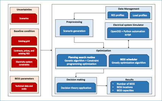
The calculation procedure is composed of two main steps, as shown in Figure 1:

(1)

Step A, essentially based on the exploitation of the features of a customized genetic algorithm, and

(2)

Step B, where the calculation of potential scheduling for all batteries installed is suggested through a greedy algorithm.

On the basis of the outputs of Step B, the objective function related to that particular set of BESSs is evaluated.

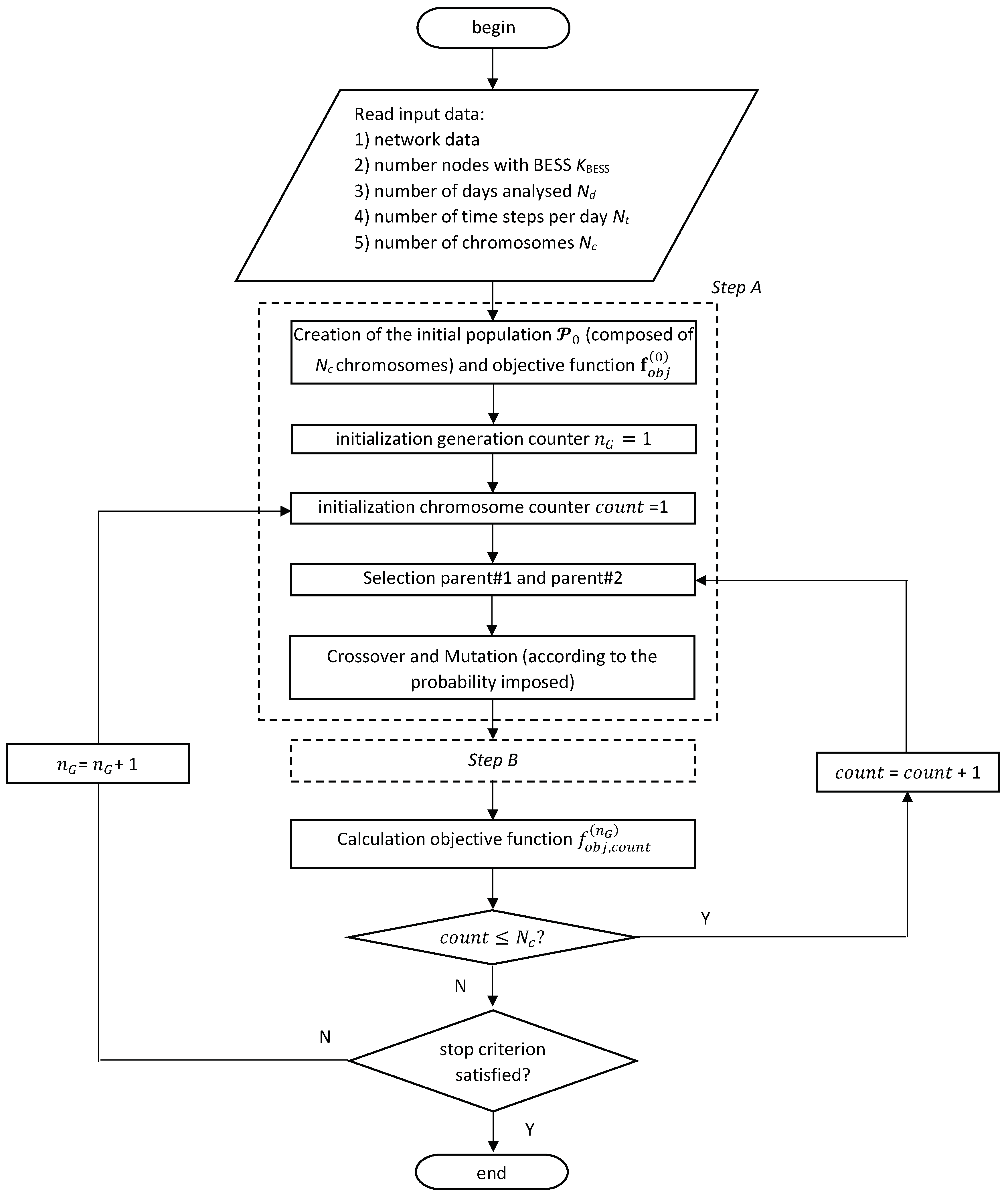
First of all, all the input data are introduced: in particular, the code requires information about the network data, number of nodes K_BESS where the BESS can be installed, time horizon (through the number of days N_d) analysed, time discretization (i.e., number of time steps per day N_t), and number of chromosomes N_c for the genetic algorithm. Thanks to the above information, the procedure continues with Step A (planning) and Step B (dispatching). After the calculation of the objective function at the iteration n_G for all the chromosomes, the convergence criterion is checked.

2.5.1. Step A

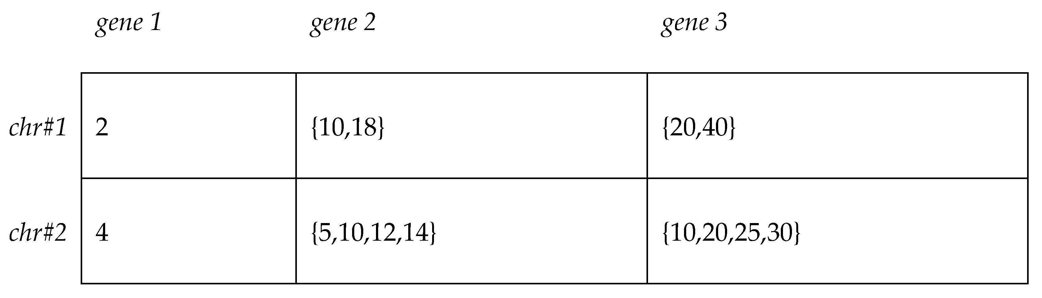
The initial population ${𝓟}_0$ is created and the initial objective function values are collected in the vector $f_{obj}^{\left(0\right)}$. The population is composed of chromosomes with the coding shown in

Table 2. Codification used in the proposed genetic algorithm.

Gene 1	Gene 2	Gene 3
Number of BESSs installed	Nodes where BESSs are installed	BESS energy capacities (kWh)

.

It is worth noting that according to the number of BESSs installed (indicated by gene 1), the number of elements composing gene 2 and gene 3 will vary. This implies that a number of pre-defined rules are needed to handle the genetic operators applied to the chromosomes, to make the creation of successive generations possible.

1. Selection and Crossover

The selection process is based on the application of the biased roulette wheel.

Once the parents’ selection is made, the crossover may be applied according to the probability of crossover p_c.

The crossover follows some general rules:

• The number of batteries is inherited from the parent#1, and
• The crossover is only applied to the values contained in gene 2 and gene 3.

Due to the particular codification used, some fixed rules have been used to apply crossover in the presence of chromosomes with different characteristics. These rules are clarified with reference to the chromosomes shown in Figure 2.

Different cases do exist:

• If parent#1 = chr#1, the offspring will be that shown in Figure 3a (offspring#1), and
• If parent#1 = chr#2, the offspring will be that shown in Figure 3b (offspring#2). In this particular case, the number of batteries imposed by parent#1 is higher than that available in parent#2. Therefore, information regarding the remaining nodes and capacities is randomly picked up from a repository containing all the nodes (and related capacities) referring to the current population (e.g., nodes {15, 24} and capacities {5, 10} in offspring#2).

2. Mutation

As the crossover operator, the mutation is only applied to the contents of gene 2 and gene 3. This operator is only applied when the value of a random number extracted from a uniform distribution is lower than the probability of mutation p_m. If the mutation is allowed, the values to be substituted are picked up from the repository containing all the nodes and relative capacities of the current population.

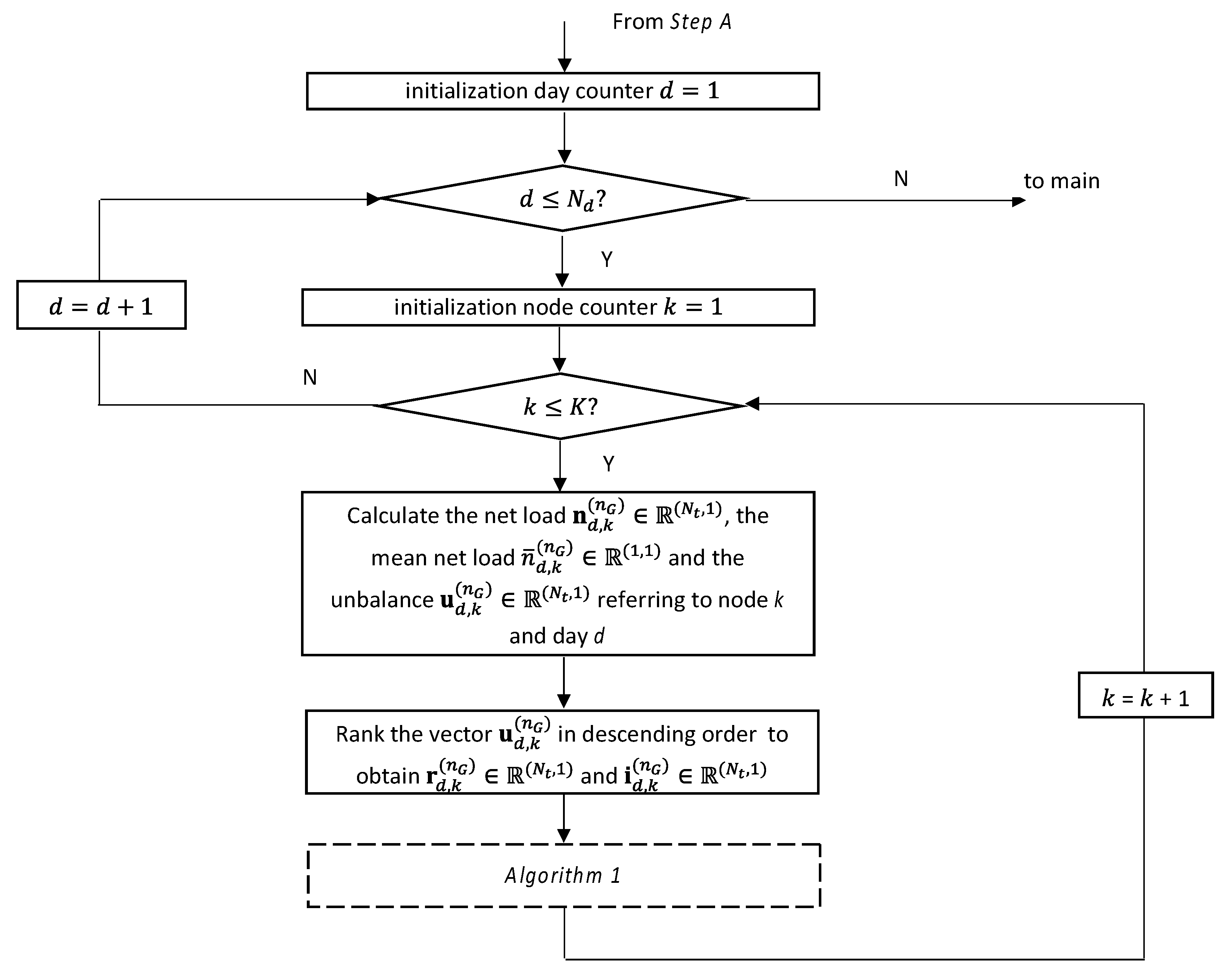
2.5.2. Step B

During Step B, the procedure calculates the operation setpoints of all the installed batteries. These setpoints are required to calculate the objective function related to the configuration (number of batteries, their positions, and their capacities) specified in every chromosome comprising the population in the generation n_G. The flow chart related to Step B is shown in Figure 4.

For every node k = 1,…,K where the batteries are installed, the net load $n_{d,k}^{\left(n_G\right)}\in {ℝ}^{\left(N_t,1\right)}$ is calculated as the difference between the load and local generation. With this information, it is possible to calculate the mean value of the nodal net load ${\overline{n}}_{d,k}^{\left(n_G\right)}\in {ℝ}^{\left(1,1\right)}$ and thus an indicative value of unbalance of the net load with respect to its mean value, i.e., $u_{d,k}^{\left(n_G\right)}\in {ℝ}^{\left(N_t,1\right)}$, calculated as

$$u_{d,k}^{\left(n_G\right)}=\left|n_{d,k}^{\left(n_G\right)}-{\overline{n}}_{d,k}^{\left(n_G\right)}\right|,k=1,\dots ,K.$$

(5)

The vector $u_{d,k}^{\left(n_G\right)}$, k = 1,…,K, provides information regarding the time steps during which the use of the battery system can be useful to level the net load.

On the basis of the value of $u_{d,k}^{\left(n_G\right)}$, the daily time steps are reordered in a descending way, by obtaining the unbalance ranked vector $r_{d,k}^{\left(n_G\right)}\in {ℝ}^{\left(N_t,1\right)}$ and the corresponding ranked index vector ${\mathsf{\nu }}_{d,k}^{\left(n_G\right)}\in {ℝ}^{\left(N_t,1\right)}$: by knowing the time steps when the unbalance is higher, it is possible to apply the scheduling algorithm by starting from the “most critical” time steps.

The pseudo-code of the scheduling algorithm is shown in Figure 5. Algorithm 1 tries to set the best option for the current time instant, which is according to the order of solving, more critical with respect to the next time instants, and pushes the battery constraint violations towards the lowest priority time steps. First of all, the set-points for a single battery (collected in the vector called $p_{BESS}^{\left(n_G\right)}$) are instructed, starting from the value of unbalance $u_{d,k}^{\left(n_G\right)}$. The feasibility of that desired pattern depends on the maximum exploitable storage level of the battery and its maximum charging power, called $P_{max}^{(-)}$, as well as its maximum discharging power $P_{max}^{(+)}$. According to the indices value collected in $r_{d,k}^{\left(n_G\right)}$, the algorithm starts from the most critical time step that is the first element of ${\mathsf{\nu }}_{d,k}^{\left(n_G\right)}$ and sets the set-point at that step by respecting the battery’s power constraint, as shown at line 5.

Then, an auxiliary variable called $I$ (that stands for integrator) is initialized at line 6 with the last value of energy stored in the battery. Following this, the integration operation is executed to check whether the energy constraint is respected or not. The parameter ω is defined as follows:

$$\omega =\{\begin{array}{ll}0,\hspace{1em}& p_{BESS,t}^{\left(n_G\right)}=NaN\\ 1,\hspace{1em}& \mathrm{else}\end{array}.$$

Line 8 indicates that a temporary value for an integral operation equal to the maximum availability state is considered at the time step t. The maximum availability state changes if either a charging or discharging mode is considered: in the discharging mode, the state is the fully charged state, whereas, in charging mode, the maximum availability state is the empty one.

Once the integration operator goes beyond the maximum and minimum state of charge ($So{C}_{max}$ and $So{C}_{min}$), a correction factor called $C_f$ resets $p_{BESS,j}^{\left(n_G\right)}$ and breaks integration execution. This operation is similarly carried out for the charging mode with corresponding signs.

2.6. Selection of the Planning Alternatives

For each scenario, the ranking of the solutions is made on the basis of the objective function (from the best solutions to the worst ones), and the Z top-ranked solutions are selected. The rationale for this selection is that there is no guarantee that the global optimum will be reached from the execution of the metaheuristic, so, taking more than one solution from the ranking, enhances the possibility of having good candidates to compare with the MCDM approach.

The number of planning alternatives is then defined as A = M × Z, that is, with the Z top-ranked solutions for each one of the M scenarios analysed.

Since each planning alternative a = 1,…,A exhibits a different performance according to the scenario, $f_{\mathrm{P}}\left(a,m\right)$ is the value of the objective function $f_{\mathrm{P}}$ defined in (2), evaluated for the alternative a when the scenario m occurs. The objective function values are then arranged into a matrix with A rows (planning alternatives) and M columns (scenarios).

The MCDM approach is based on the application of decision theory criteria to the A planning alternatives by considering the M scenarios. In the framework of the decision theory concepts, several criteria can be applied to select the optimal planning alternative, taking into account that each scenario m has a probability of occurrence p_m.

2.6.1. Criterion of Minimum Expected Cost

The criterion of the minimum expected cost attempts to minimize the costs [33]. The optimal planning alternative $a_{ec}^{*}$ is the one that minimizes the expected cost EC:

$$a_{ec}^{*}=\underset{a=1,\dots ,A}{\arg \min }\left\{EC\left(a\right)\right\},$$

(6)

where the expected cost EC$\left(a\right)$ for each alternative a = 1,…,A is determined as

$$EC\left(a\right)={{\displaystyle \sum }}_{m=1}^M{p}_m{f}_p\left(a,m\right).$$

(7)

The assignment of the probabilities of occurrence is crucial; when the equal likelihood criterion is adopted [34], each scenario has the same probability of occurrence.

2.6.2. Criterion of Minimax Weighted Regret

The criterion of minimax weighted regret attempts to minimize the regret corresponding to the worst case [34]. For a given scenario m, it is possible to identify the best planning alternative as the one corresponding to the lowest cost; if a planning alternative different from the optimal one is chosen, a greater cost will be experienced and, therefore, the regret can be calculated. Let us consider the scenario m, where the best planning alternative $a_m^{*}$ is

$$a_m^{*}=\underset{a=1,\dots ,A}{\arg \min }\left\{f_p\left(a,m\right)\right\}$$

(8)

and, when scenario m occurs and the alternative a different from $a_m^{*}$ is chosen, the regret can be quantified as

$$R\left(a,m\right)=f_p\left(a,m\right)-f_p\left(a_m^{*},m\right).$$

(9)

Considering the probability of occurrence of each scenario, the weighted regret $R_w\left(a,m\right)$ is determined as

$$R_w\left(a,m\right)=p_{m}R\left(a,m\right).$$

(10)

According to the criterion of minimax weighted regret, the optimal planning alternative $a_{wr}^{*}$ is the one that minimizes the maximum weighted regret, that is,

$$a_{wr}^{*}=\underset{a=1,\dots ,A}{\arg \min }\left\{\underset{m=1,\dots M}{\max }\left(R_w\left(a,m\right)\right)\right\}.$$

(11)

As in the case of the criterion of Section 2.6.1, the equal likelihood criterion can be adopted [33].

2.6.3. “Optimist” and “Pessimist”Criterion

When the “optimist” criterion is applied [28,31], for each planning alternative, the best value of the costs (i.e., the minimum value) over the possible scenarios is selected and, then, the selected planning alternative $a_{opt}^{*}$ is the one that minimizes the cost corresponding to the best possible outcome for each scenario, that is,

$$a_{opt}^{*}=\underset{a=1,\dots ,A}{\arg \min }\left\{\underset{m=1,\dots M}{\min }{f}_p\left(a,m\right)\right\}.$$

(12)

Conversely, the “pessimist” criterion [28,31] attempts to minimize the worst outcome of the planning alternatives. Therefore, the worst value of the costs (i.e., the maximum value) of each alternative over the possible scenarios is selected and, then, the selected planning alternative $a_{pes}^{*}$ is the one that minimizes the worst outcome, that is,

$$a_{pes}^{*}=\underset{a=1,\dots ,A}{\arg \min }\left\{\underset{m=1,\dots M}{\max }{f}_p\left(a,m\right)\right\}.$$

(13)

In addition, an “optimist”-“pessimist” criterion can be considered as a mixed approach. In this case, both the worst and best outcome of each alternative are considered and these values are weighted by a proper factor $\alpha \in \left[0,1\right]$:

$$a_{opt-pes}^{*}=\underset{a=1,\dots ,A}{\arg \min }\left\{\alpha \underset{m=1,\dots M}{\min }{f}_p\left(a,m\right)+\left(1-\alpha \right)\underset{m=1,\dots M}{\max }{f}_p\left(a,m\right)\right\}.$$

(14)

When applying the “optimist”, the “pessimist”, and the “optimist”-“pessimist” criteria, the decision does not depend on the probabilities of the scenarios.

3. Case Study Application and Results

3.1. Network Data

The application presented in this paper is based on a rural LV network with 22 nodes, including the slack node (Figure 6). The network is radial and is supplied by the MV system through an MV/LV transformer (not represented in the figure). The network contains mainly residential and agricultural customers. The number of nodes considered for BESS installation is $K_{\mathrm{BESS}}$ = 5. The BESS data are shown in

Table 3. Battery Energy Storage System (BESS) capacity data.

Minimum Energy Capacity (kWh)	Maximum Energy Capacity (kWh)	Discretization Steps	Energy to Power Ratio
3	49	47	2

. For discretization of the BESS energy capacity, the number of levels used is $\Lambda$ = 47, with BESS energy capacities considered to lie in the range 3 ÷ 49 kWh, and the energy to power ratio is equal to 2, as indicated in Section 2.3 [29]. The total number of alternative combinations of BESS sizes is $S={\Lambda }^{K_{\mathrm{BESS}}}$ = 47⁵ = 2.29 × 10⁸. Such a number is practically intractable with an exhaustive search process. In this situation, the use of a metaheuristic algorithm to identify the solution of the planning problem is justified.

3.2. Input Data

Without loss of generality, the reference period T_ref is assumed to be one year, and the planning time horizon is assumed to be 15 years (i.e., N_H = 15).

The batteries chosen are Lithium Ion (type Nickel Manganese Cobalt): the cost used in this paper is the one expected in 2020 and equal to 167 $/kWh, whereas the inverter cost is equal to 50 $/kW. The operation and maintenance cost is equal to 1% of the investment cost per year. The BESS lifetime has been considered to be equal to 13.4 years [29]. The BESS degradation has been modeled as a reduction of the energy capacity of the battery, equal to 2.4% per year [35].

For execution of the genetic algorithm, the probability of crossover is imposed as p_c = 0.75, and the probability of mutation is set to p_m = 0.05.

3.2.1. Loads

Regarding the calculation of the load profiles, it takes into account the real contractual delivery powers of each load. Two nodes are considered as commercial consumers, while the other ones refer to residential customers. For the profiles, due to a lack of complete information from the actual profiles, relevant (residential and commercial) profiles have been taken from an open-source dataset (OpenEI) [36], normalized and multiplied by the nominal powers.

3.2.2. PV Generation

The considered PV production, in the simulation, is calculated based on yearly solar irradiance and the nominal installed power [37]. Yearly solar irradiance data was obtained through collected data from a third party weather service provider [38] for the specific location of the case study with the coordinates of 46.4746° N, 11.2479° E.

3.2.3. EV Relevant Information

EVs are considered in some scenarios, through the load profile caused by their charging. Within this analysis, the number of EVs that determines the EV charging profile is set to 10 at the beginning of the scenarios with EV and that number gradually increases by the rate of one EV per year. The nominal power of the EV chargers is considered to be 3.6 kW, i.e., a standard power level of charging stations, and charging events mainly occur during the night.

3.2.4. Energy Price Evolution

Energy price evolutions increase and decrease linearly, with the granularity of one year along entire scenario horizons.

3.3. Definition of the Scenarios

The scenarios are defined by assuming the following entries:

(a)

Electricity prices: M_P = 2 trends of variation are considered, namely, with a 50% increase and 20% reduction of the prices in the planning time horizon of 20 years. Linear variations of the prices are assumed during the years;

(b)

Diffusion of the local generation: M_DG = 2 trends of variation of the local generation are considered, with a 20% and 50% increase of the energy production from local generation in the planning time horizon of 20 years. Linear variations of the local generation diffusion are assumed during the years;

(c)

Diffusion of charging points for electric vehicles: M_EV = 2 trends are assumed, in which (i) no parking lot and no battery charging stations will be built, and (ii) one parking lot considering 10 active (i.e., with an EV connected for charging purposes) charging points at node 13 is assumed, with the increase rate of the number of active charging points of 1 per year.

3.4. Calculation of the Objective Function

The objective function has been evaluated for each planning alternative and scenario. The best three solutions for each one of the eight scenarios have been calculated for all the scenarios to provide the starting matrix to carry out the calculations based on decision theory. The number of alternatives is then 24.

Table 4. Values of the objective function for each planning alternative and for each scenario (×10¹²). Values in bold indicate the best solution for each scenario.

	Scenarios
Alternative	1	2	3	4	5	6	7	8
1	0.373	0.600	2.44	3.39	5.98	8.31	16.7	23.2
2	0.371	0.515	1.78	2.47	5.84	8.10	16.3	22.6
3	0.371	0.514	1.78	2.47	5.83	8.10	16.3	22.6
4	0.381	0.529	2.07	2.88	5.15	7.15	16.5	22.9
5	0.351	0.543	1.78	2.47	5.46	7.58	16.2	22.5
6	0.393	0.545	2.09	2.90	5.55	7.71	16.9	23.5
7	0.412	0.572	1.38	1.92	5.65	7.84	14.2	19.8
8	0.370	0.514	1.39	1.93	5.82	8.08	14.6	20.3
9	0.431	0.598	1.39	1.92	6.00	8.33	13.5	18.7
10	0.366	0.601	1.49	2.07	5.97	8.29	14.8	20.6
11	0.366	0.628	1.45	2.01	5.97	8.28	14.3	19.9
12	0.350	0.514	1.78	2.10	5.97	8.29	15.0	20.8
13	0.406	0.564	2.20	3.06	5.22	7.24	17.0	23.6
14	0.433	0.601	1.73	2.41	5.18	8.31	15.7	21.8
15	0.432	0.600	1.74	2.42	5.35	8.31	15.8	22.0
16	0.402	0.559	2.19	3.04	5.17	7.17	16.9	23.4
17	0.404	0.561	2.12	2.94	5.19	7.21	16.1	22.3
18	0.402	0.559	2.20	3.06	5.49	7.62	17.0	23.6
19	0.378	0.525	1.75	2.43	5.13	7.12	16.5	23.0
20	0.404	0.561	1.28	1.78	5.24	7.28	14.7	20.4
21	0.431	0.598	1.91	2.65	5.96	8.28	16.5	22.9
22	0.348	0.567	1.46	2.03	5.84	8.11	14.9	20.6
23	0.351	0.600	1.80	2.50	5.96	8.28	15.8	21.9
24	0.366	0.602	2.20	3.05	5.99	8.31	17.0	23.6

shows the objective function values: it is worth noting that, with respect to scenario 2, the values of the objective function for alternatives 3, 8, and 12 are 0.5135, 0.5136, and 0.5140, respectively. Scenarios 5–8 (associated with a large deployment of EVs) exhibit higher values of the objective function.

Table 5. Technical data of the planning alternatives.

Alternative	Number of BESSs	Nodes	Energy Capacity (kWh)
1	1	14	21
2	2	0, 18	23, 49
3	2	15, 18	39, 49
4	2	10, 11	47, 12
5	2	18, 20	36, 40
6	2	20, 13	28, 11
7	3	14, 17, 10	21, 42, 9
8	2	11, 18	3, 47
9	3	7, 11, 17	34, 36, 19
10	2	9, 17	28, 40
11	2	17, 16	38, 21
12	2	8, 18	24, 34
13	1	10	29
14	1	19	38
15	1	19	21
16	3	10, 1, 8	36, 6, 18
17	2	10, 7	32, 28
18	2	10, 12	15, 43
19	2	13, 10	42, 16
20	2	10, 17	28, 45
21	3	17, 8, 0	12, 49, 16
22	3	13, 17, 8	13, 41, 20
23	3	8, 17, 8	16, 23, 49
24	3	9, 8, 0	15, 49, 28

reports the technical data of the alternatives, including the number of BESSs installed, the nodes where each BESS is located, and the BESS energy capacity at each node. The solutions include one to three BESSs. Looking at the BESS locations, it can be seen that, in three cases, the slack node is chosen to install a BESS. In this way, the BESS acts to limit the reverse power flows. In the alternative number 23, node 8 is selected two times, because the energy capacity of the BESS in one installation reaches the limits, and the procedure did not find a better alternative to place the BESS in another node.

3.5. Decision Theory-Based Assessment of the Planning Alternatives and Scenarios

Several cases have been considered, with different values of probability of occurrence assigned to each scenario (

Table 6. Values of scenario probabilities.

	Case 1	Case 2	Case 3	Case 4	Case 5	Case 6	Case 7
Scenario 1	0.125	0.05	0.20	0.05	0.20	0.05	0.15
Scenario 2	0.125	0.20	0.05	0.05	0.20	0.15	0.05
Scenario 3	0.125	0.05	0.20	0.05	0.20	0.05	0.15
Scenario 4	0.125	0.20	0.05	0.05	0.20	0.25	0.05
Scenario 5	0.125	0.05	0.20	0.20	0.05	0.05	0.25
Scenario 6	0.125	0.20	0.05	0.20	0.05	0.15	0.05
Scenario 7	0.125	0.05	0.20	0.20	0.05	0.05	0.25
Scenario 8	0.125	0.20	0.05	0.20	0.05	0.25	0.05

). In Case 1, all scenarios have the same probability of occurrence and, then, the equal likelihood criterion is considered. Cases 2 and 3 consider that it is more probable that the scenarios with higher and lower price increases will occur, respectively. Cases 4 and 5 are focused on the deployment of EVs. In particular, in Case 4, the scenarios with the large deployment of EVs are weighted more, while in Case 5, the scenarios with no deployment of EVs are weighted more. In Case 6, the probabilities are higher for scenarios with a higher price increase and higher PV installation. Finally, Case 7 weights the scenarios with a lower price increase and large deployment of EVs more.

3.5.1. Application of the Criterion of the Minimum Expected Cost

Table 7. Expected costs (×10¹²). Values in bold indicate the best solution for each case.

Alternative	Case 1	Case 2	Case 3	Case 4	Case 5	Case 6	Case 7
1	7.61	8.36	6.87	11.2	4.07	9.24	7.86
2	7.24	7.94	6.53	10.8	3.67	8.76	7.53
3	7.24	7.94	6.53	10.8	3.66	8.76	7.53
4	7.20	7.91	6.50	10.6	3.76	8.81	7.46
5	7.12	7.82	6.42	10.6	3.62	8.66	7.40
6	7.45	8.18	6.73	11.0	3.87	9.09	7.73
7	6.47	7.10	5.84	9.71	3.23	7.77	6.75
8	6.63	7.28	5.99	10.0	3.28	7.96	6.92
9	6.35	6.97	5.73	9.51	3.19	7.55	6.61
10	6.78	7.45	6.11	10.2	3.39	8.13	7.06
11	6.62	7.27	5.97	9.92	3.32	7.92	6.89
12	6.86	7.50	6.21	10.3	3.45	8.21	7.15
13	7.41	8.14	6.69	10.9	3.90	9.08	7.67
14	7.02	7.78	6.27	10.5	3.58	8.54	7.20
15	7.08	7.83	6.34	10.6	3.61	8.60	7.29
16	7.36	8.07	6.64	10.8	3.87	9.01	7.61
17	7.11	7.80	6.41	10.5	3.75	8.67	7.35
18	7.48	8.21	6.75	11.0	3.93	9.14	7.75
19	7.11	7.80	6.41	10.6	3.61	8.69	7.39
20	6.45	7.08	5.82	9.71	3.18	7.79	6.73
21	7.40	8.12	6.68	11.0	3.80	8.96	7.68
22	6.73	7.39	6.07	10.1	3.35	8.09	7.01
23	7.15	7.86	6.45	10.7	3.65	8.63	7.43
24	7.64	8.39	6.89	11.3	3.99	9.28	7.91

reports the expected costs for each alternative in all cases considered. From the values of the expected costs, the selected planning alternative is Alternative 9 for cases 1–4 and 6–7. Alternative 9 is characterized by lower costs in scenarios 7 and 8 (generally associated with high values of costs); as such, it is often the selected alternative. The criterion of the minimum expected cost provides Alternative 20 as the preferred one in Case 5, when scenarios 1–4 are more weighted.

3.5.2. Application of the Minimax Weighted Regret Criterion

Table 8. Maximum weighted regrets (×10¹²). Values in bold indicate the best solution for each case.

Alternative	Case 1	Case 2	Case 3	Case 4	Case 5	Case 6	Case 7
1	0.560	0.896	0.644	0.896	0.322	1.120	0.805
2	0.486	0.778	0.560	0.778	0.195	0.973	0.700
3	0.486	0.778	0.560	0.778	0.194	0.972	0.700
4	0.534	0.854	0.615	0.854	0.219	1.068	0.768
5	0.483	0.773	0.556	0.773	0.193	0.966	0.696
6	0.605	0.967	0.696	0.967	0.242	1.209	0.870
7	0.136	0.218	0.157	0.218	0.055	0.273	0.196
8	0.206	0.330	0.238	0.330	0.083	0.413	0.297
9	0.151	0.241	0.174	0.241	0.060	0.181	0.217
10	0.242	0.386	0.278	0.386	0.097	0.483	0.347
11	0.154	0.247	0.177	0.247	0.062	0.308	0.221
12	0.270	0.431	0.310	0.431	0.108	0.539	0.388
13	0.617	0.988	0.710	0.988	0.255	1.235	0.888
14	0.391	0.626	0.450	0.626	0.156	0.782	0.562
15	0.413	0.661	0.475	0.661	0.165	0.826	0.593
16	0.596	0.953	0.686	0.953	0.253	1.191	0.857
17	0.457	0.732	0.527	0.732	0.233	0.915	0.658
18	0.612	0.979	0.705	0.979	0.255	1.224	0.881
19	0.537	0.859	0.618	0.859	0.215	1.074	0.772
20	0.212	0.339	0.244	0.339	0.085	0.424	0.305
21	0.527	0.843	0.607	0.843	0.211	1.054	0.759
22	0.243	0.388	0.279	0.388	0.097	0.486	0.349
23	0.406	0.650	0.468	0.650	0.162	0.812	0.585
24	0.616	0.985	0.710	0.985	0.254	1.232	0.887

reports the maximum weighted regrets for each alternative in all cases considered.

From the values of the maximum weighted regrets, the selected planning alternative is Alternative 7, for cases 1–5 and 7. The values of the objective function in scenarios with a large deployment of EVs influence the results also for this criterion, as in 3.5.1.

3.5.3. Application of the “Optimist-Pessimist”Criterion

The “optimist-pessimist” criterion was applied, considering different values of the weighting factor $\alpha$ ranging from 0 to 1. The case with $\alpha$ = 0 corresponds to the application of the “pessimist” criterion, while the case with $\alpha$ = 1 is equal to the application of the “optimistic” criterion. The results are reported in

Table 9. Selected planning alternatives obtained by applying the “optimist-pessimist” criterion.

α	Selected Planning Alternative
0.0	9
0.1	9
0.2	9
0.3	9
0.4	9
0.5	9
0.6	9
0.7	9
0.8	9
0.9	9
1.0	22

.

From these results, Alternative 9 is the selected alternative for all the values of the weighting factor, with the exception of the case with $\alpha$ = 1. The “optimistic” criterion ($\alpha$ = 1) selects Alternative 22, which is associated with the lowest value of the objective function; for the other values of the weighting factor $\alpha$, higher values of the objective function in scenarios 7–8 influence the results.

4. Conclusions

This paper has presented a novel procedure that combines planning and scheduling of the BESSs installed in an LV grid. In this way, BESS siting and sizing is carried out with the support of a specific assessment of the system operation. The proposed approach combines the properties of the metaheuristics used to search for solutions in a wide space (for the creation of planning alternatives) and the fast calculation of the greedy procedure that allows a viable solution to be found for BESS scheduling. This approach makes it possible to overcome the limitation due to the intractable total number of combinations of BESS sizes, simultaneously handling the non-trivial operational aspects linked to variations in time of the power flows in the network and the BESS scheduling. Furthermore, the uncertainty regarding future scenarios has been handled with a decision theory-based method.

Alternatives 7 and 9 have emerged as the most promising ones when using the decision theory criteria. In particular, Alternative 9 has been preferred by the expected costs and the “optimist-pessimist” criteria, in quite a robust way, over most of the cases with weighted scenarios. Alternative 7 has been preferred by the minimax weighted regrets criterion, again over most of the cases with weighted scenarios. In these two alternatives, three nodes are chosen for BESS installation (with node 17 in common) and the BESS sizes in these nodes are intermediate with respect to the minimum and maximum energy capacity limits used. For a problem of this kind, there can be no guarantee that a globally optimal solution has been reached. For this reason, the creation of meaningful scenarios taking into account the local conditions of loads and generation becomes a fundamental aspect that can be successfully addressed in the case of relatively small electricity communities, where the energy community manager may have an easier view on the decision variables involved in the system operation and planning with respect to what occurs in larger systems. To further develop scenarios of local loads and generation, future research will consider the deployment of other electrification technologies, like heat pumps, that can significantly impact the demand; it will also consider the inclusion of three-phase or single-phase PV systems with storage to take into account the trend of the prosumers to install storage systems in their local plants with the aim of increasing self-sufficiency.

References

1. Zidar, M.; Georgilakis, P.S.; Hatziargyriou, N.D.; Capuder, T.; Škrlec, D. Review of energy storage allocation in power distribution networks: Applications, methods and future research. IET Gener. Transm. Distrib. 2016, 10, 645–652. [Google Scholar] [CrossRef]
2. Boicea, V.A. Energy Storage Technologies: The Past and the Present. Proc. IEEE 2014, 102, 1778–1794. [Google Scholar] [CrossRef]
3. Chen, S.; Zhang, T.; Gooi, H.B.; Masiello, R.D.; Katzenstein, W. Penetration rate and effectiveness studies of aggregated BESS for frequency regulation. IEEE Trans. Smart Grid 2016, 7, 167–177. [Google Scholar] [CrossRef]
4. Brogan, P.V.; Best, R.J.; Morrow, D.J.; McKinley, K.; Kubik, M.L. Effect of BESS response on frequency and RoCof during underfrequency transients. IEEE Trans. Power Syst. 2019, 34, 575–583. [Google Scholar] [CrossRef] [Green Version]
5. Brivio, C.; Mandelli, S.; Merlo, M. Battery energy storage system for primary control reserve and energy arbitrage. Sustain. Energy Grids Netw. 2016, 6, 152–165. [Google Scholar] [CrossRef]
6. Mosca, C.; Arrigo, F.; Mazza, A.; Bompard, E.; Carpaneto, E.; Chicco, G.; Cuccia, P. Mitigation of Frequency Stability Issues in Low Inertia Power Systems using Synchronous Compensators and Battery Energy Storage Systems. IET Gener. Transm. Distrib. 2019, 13, 3951–3959. [Google Scholar] [CrossRef]
7. Zheng, Y.; Dong, Z.Y.; Luo, F.J.; Meng, K.; Qiu, J.; Wong, K.P. Optimal Allocation of Energy Storage System for Risk Mitigation of DISCOs with High Renewable Penetrations. IEEE Trans. Power Syst. 2014, 29, 212–220. [Google Scholar] [CrossRef]
8. Qiu, J.; Xu, Z.; Zheng, Y.; Wang, D.; Dong, Z.Y. Distributed generation and energy storage system planning for a distribution system operator. IET Renew. Power Gener. 2018, 12, 1345–1353. [Google Scholar] [CrossRef]
9. Saboori, H.; Hemmati, R.; Sadegh Ghiasi, S.M.; Dehghan, S. Energy storage planning in electric power distribution networks—A state-of-the-art review. Renew. Sustain. Energy Rev. 2017, 79, 1108–1121. [Google Scholar] [CrossRef]
10. Alegria, E.; Brown, T.; Minear, E.; Lasseter, R.H. CERTS Microgrid Demonstration with Large-Scale Energy Storage and Renewable Generation. IEEE Trans. Smart Grid 2014, 5, 937–943. [Google Scholar] [CrossRef]
11. Zheng, Y.; Zhao, J.; Song, Y.; Luo, F.; Meng, K.; Qiu, J.; Hill, D.J. Optimal Operation of Battery Energy Storage System Considering Distribution System Uncertainty. IEEE Trans. Sustain. Energy 2018, 9, 1051–1060. [Google Scholar] [CrossRef]
12. Hussain, A.; Bui, V.-H.; Kim, H.M. Impact Analysis of Demand Response Intensity and Energy Storage Size on Operation of Networked Microgrids. Energies 2017, 10, 882. [Google Scholar] [CrossRef] [Green Version]
13. Kumar, A.; Meena, N.K.; Singh, A.R.; Deng, Y.; Kumar, P. Strategic integration of battery energy storage systems with the provision of distributed ancillary services in active distribution systems. Appl. Energy 2019, 253, 113503. [Google Scholar] [CrossRef]
14. Sedghi, M.; Ahmadian, A.; Aliakbar-Golkar, M. Optimal Storage Planning in Active Distribution Network Considering Uncertainty of Wind Power Distributed Generation. IEEE Trans. Power Syst. 2016, 31, 304–316. [Google Scholar] [CrossRef]
15. Ahmadian, A.; Sedghi, M.; Aliakbar-Golkar, M. Fuzzy Load Modeling of Plug-in Electric Vehicles for Optimal Storage and DG Planning in Active Distribution Network. IEEE Trans. Veh. Technol. 2017, 66, 3622–3631. [Google Scholar] [CrossRef]
16. Wong, L.A.; Ramachandaramurthy, V.K.; Taylor, P.; Ekanayake, J.B.; Padmanaban, S. Review on the optimal placement, sizing and control of an energy storage system in the distribution network. J. Energy Storage 2019, 21, 489–504. [Google Scholar] [CrossRef]
17. Andreotti, A.; Carpinelli, G.; Mottola, F.; Proto, D.; Russo, A. Decision Theory Criteria for the Planning of Distributed Energy Storage Systems in the Presence of Uncertainties. IEEE Access 2018, 6, 62136–62151. [Google Scholar] [CrossRef]
18. Tang, Z.; Liu, J.; Liu, Y.; Huang, Y.; Jawad, S. Risk awareness enabled sizing approach for hybrid energy storage system in distribution network. IET Gener. Transm. Distrib. 2019, 13, 3814–3822. [Google Scholar] [CrossRef]
19. Pavić, I.; Luburić, A.; Pandžić, H.; Capuder, T.; Andročec, I. Defining and Evaluating Use Cases for Battery Energy Storage Investments: Case Study in Croatia. Energies 2019, 12, 376. [Google Scholar] [CrossRef] [Green Version]
20. Yunusov, T.; Frame, D.; Holderbaum, W.; Potter, B. The impact of location and type on the performance of low-voltage network connected battery energy storage systems. Appl. Energy 2016, 165, 202–213. [Google Scholar] [CrossRef] [Green Version]
21. Giannitrapani, A.; Paoletti, S.; Vicino, A.; Zarrilli, D. Optimal Allocation of Energy Storage Systems for Voltage Control in LV Distribution Networks. IEEE Trans. Smart Grid 2017, 8, 2859–2870. [Google Scholar] [CrossRef]
22. Crossland, A.F.; Jones, D.; Wade, N.S. Planning the location and rating of distributed energy storage in LV networks using a genetic algorithm with simulated annealing. Int. J. Electr. Power Energy Syst. 2014, 59, 103–110. [Google Scholar] [CrossRef] [Green Version]
23. Jannesar, M.R.; Sedighi, A.; Savaghebi, M.; Guerrero, J.M. Optimal placement, sizing, and daily charge/discharge of battery energy storage in low voltage distribution network with high photovoltaic penetration. Appl. Energy 2018, 226, 957–966. [Google Scholar] [CrossRef] [Green Version]
24. Fortenbacher, P.; Ulbig, A.; Andersson, G. Optimal Placement and Sizing of Distributed Battery Storage in Low Voltage Grids Using Receding Horizon Control Strategies. IEEE Trans. Power Syst. 2018, 33, 2383–2394. [Google Scholar] [CrossRef] [Green Version]
25. Khalid Mehmood, K.; Khan, S.U.; Lee, S.; Haider, Z.M.; Rafique, M.K.; Kim, C. Optimal sizing and allocation of battery energy storage systems with wind and solar power DGs in a distribution network for voltage regulation considering the lifespan of batteries. IET Renew. Power Gener. 2017, 11, 1305–1315. [Google Scholar] [CrossRef]
26. Babacan, O.; Torre, W.; Kleissl, J. Optimal allocation of battery energy storage systems in distribution networks considering high PV penetration. In Proceedings of the 2016 IEEE Power and Energy Society General Meeting (PESGM), Boston, MA, USA, 17–21 July 2016. [Google Scholar]
27. Carpinelli, G.; Mottola, F.; Proto, D.; Russo, A.; Varilone, P. A Hybrid Method for Optimal Siting and Sizing of Battery Energy Storage Systems in Unbalanced Low Voltage Microgrids. Appl. Sci. 2018, 8, 455. [Google Scholar] [CrossRef] [Green Version]
28. French, S. Decision Theory, an Introduction to the Mathematics of Rationality; Ellis Horwood: Chichester, UK, 1989. [Google Scholar]
29. IRENA. Electricity Storage and Renewables: Costs and Markets to 2030; October 2017; ISBN 978-92-9260-038-9. Available online: https://www.irena.org/publications/2017/Oct/Electricity-storage-and-renewables-costs-and-markets (accessed on 17 December 2019).
30. Von Appen, J.; Braun, M.; Stetz, T.; Diwold, K.; Geibel, D. Time in the sun: The challenge of high PV penetration in the German electric grid. IEEE Power Energy Mag. 2013, 11, 55–64. [Google Scholar] [CrossRef]
31. Mortazavi, H.; Mehrjerdi, H.; Saad, M.; Lefebvre, S.; Asber, D.; Lenoir, L. A monitoring technique for reversed power flow detection with high PV penetration level. IEEE Trans. Smart Grid 2015, 6, 2221–2232. [Google Scholar] [CrossRef]
32. De Carne, G.; Buticchi, G.; Zou, Z.; Liserre, M. Reverse Power Flow Control in a ST-Fed Distribution Grid. IEEE Trans. Smart Grid 2018, 9, 3811–3819. [Google Scholar] [CrossRef]
33. Anders, G.J. Probability Concepts in Electric Power Systems; John Wiley & Sons: New York, NY, USA, 1990. [Google Scholar]
34. Miranda, V.; Proenca, L.M. Probabilistic choice vs. risk analysis-conflicts and synthesis in power system planning. IEEE Trans. Power Syst. 1998, 13, 1038–1043. [Google Scholar] [CrossRef]
35. Kubiak, P.; Cen, Z.; Lόpez, C.M.; Belharouak, I. Calendar aging of a 250 kW/500 kWh Li-ion battery deployed for the grid storage application. J. Power Sources 2017, 372, 16–23. [Google Scholar] [CrossRef]
36. OpenEI. Available online: https://openei.org/datasets/files/961/pub/ (accessed on 17 December 2019).
37. Spertino, F.; Corona, F.; Di Leo, P. Limits of Advisability for Master–Slave Configuration of DC–AC Converters in Photovoltaic Systems. IEEE J. Photovolt. 2012, 2, 547–554. [Google Scholar] [CrossRef]
38. World Weather Online. Available online: https://www.worldweatheronline.com/ (accessed on 17 December 2019).
Figure 1. Scheme of the proposed procedure.
Energies 13 00052 g001
Figure 2. Example of chromosomes.
Energies 13 00052 g002
Figure 3. Example of offpring when the parents have different lengths.
Energies 13 00052 g003
Figure 4. Flowchart related to Step B.
Energies 13 00052 g004
Figure 5. Pseudo-code of the battery scheduling.
Energies 13 00052 g005
Figure 6. Rural LV network.
Energies 13 00052 g006