1. Introduction
Friction brakes are used to convert the kinetic, and sometimes potential energy of the vehicle, into thermal energy, hence, allowing the vehicle to decelerate or stop when required. Since brakes can generate a substantial amount of heat energy in a short instance, overheating of the brake discs is a possible scenario to be avoided. Overheating can cause brake fading, brake judder, increased wear, as well as thermal cracking and even brake fluid vaporization [
1,
2], which constitutes a serious safety issue. Furthermore, other parts of wheel suspension, wheel cover or tire, can also be affected by high temperatures, especially during the thermal soak process [
3,
4].
In order to avoid brake system overheating, it is a necessity that the brake assembly is appropriately dimensioned and designed as to store and dissipate energy without reaching critical temperatures, even in the most extreme braking scenarios. Traditionally, the brake systems have been tested experimentally using different test benches, such as full-scale brake dynamometer, as well as through complete vehicle testing. However, nowadays, some tests can be replicated by CAE simulations, which are cheaper and can also provide information difficult to obtain in real life tests. Moreover, the simulations can be performed at much earlier stages, such as concept phase, hence, avoiding possible later problems in vehicle development, reducing both prototyping costs and lead time for parts and by that reducing the total length of vehicle development.
The complexity of the computer-aided design (CAD) models for numerical simulations can vary significantly. Simple studies looked into modelling of a single channel inside the brake disc [
5], a sector of the brake disc [
6,
7] or just the brake disc with some surrounding geometries [
8,
9,
10]. More complex studies would include more geometrical parts [
11,
12], which have been shown to be more representative of the on-road conditions [
11]. At the same time, from the physics perspective, these simulations would often focus either on computing convection heat transfer coefficients from a computational fluid dynamics (CFD) point of view or on conduction modelling through the solid parts. Simulations that include both effects are more challenging and demanding in terms of setup since they require coupling between fluid and thermal solvers to account for changes in both flow and temperature fields [
12,
13,
14].
Complete replacement of the brake cooling experimental tests by numerical simulations is a demanding task as it requires accurate modelling of all three heat transfer mechanisms: convection (through airflow passing inside and around the disc), conduction (through the support and contact areas) and, at last, radiation. This paper addresses the complexity of this modelling and discusses simplifications and limitations that need to be accounted for.
2. Complications of Modelling Aero-Thermal Problems
Several different tests are usually performed to ensure the correct brakes system cooling performance, some of them last several minutes and some can last much longer. Moreover, the dominant heat transfer mechanism would differ depending on the test scenario.
Convection is usually the most important mechanism for cooling. Radiation is important only for high temperatures, such as a glowing brake disc. The contribution of conduction through the support is less important since it is a slow process [
10]; however, it will be dominant if the test includes the soaking phase when the vehicle is stopped and forced convection is replaced by natural convection. Nevertheless, all these mechanisms need to be modelled for every test scenario if the test results are to be replicated accurately.
Historically, CFD codes were used to compute convection heat transfer coefficients (HTCs), while separate thermal solvers were used to model conduction and radiation [
12,
13,
15]. Specifics of aerodynamic and thermal models are discussed in later chapters; here, the focus is on the coupling process and data exchange between different solvers. It should be noted that there are studies that combine fluid and solid domains within the same finite volume solver [
16]; however, they still experience most of the issues presented in this paper.
2.1. Coupling Approaches
The data exchange process between two models, also known as coupling, usually involves transferring HTCs and reference fluid temperatures from aerodynamic solver to the thermal solver. The thermal solver uses these data to estimate the convection heat fluxes for part surfaces and combines it with computed conduction and radiation fluxes to estimate the changes in components temperatures during a specified time period. New surface temperatures are then being transferred to the aerodynamic solver for recalculating the airflow around the simulated components, see
Figure 1.
The communication between two separate solvers can be set up in several different ways. The most accurate method would be to use a fully-transient approach when changes in the airflow and HTCs are continuously modelled for the whole duration of the test. However, simulating several minutes of the transient airflow around the vehicle can be extremely expensive in terms of computational resources; therefore, other simulation approaches have been developed.
One of the popular approaches is to consider the flow around the rotating brake disc to be independent of the surface temperatures. This assumption allows performing only a few aerodynamic simulations with different vehicle velocities. Interpolation is then used to obtain surface HTC dependency curves for all vehicle velocities. These curves are then used in the thermal model without any additional flow recalculation loops required. Such simplification works relatively well for high speed scenarios [
13]; however, if the simulated vehicle velocities are slow, the buoyancy effects become more pronounced, and this approach thereby becomes invalid.
More accurate simulation approaches, usually referred to as “semi-transient”, use two-way coupling between thermal and aerodynamic solvers, i.e., the airflow and HTCs are being updated several times during one simulation. In this case, surface HTCs are considered dependent on both the vehicle velocity and component surface temperatures.
An important parameter for semi-transient simulations is the coupling frequency. Some approaches would assume a step curve for HTCs of the parts and require frequent recalculations of them, while others would assume linear behaviour of the surface HTCs and, hence, allow much longer time intervals between coupling [
13,
14,
17]. Both methods have pros and cons, depending on the test scenario being simulated.
2.2. Data Mapping
Addressing the complications of a coupling process, it is important to remember the data mapping between codes. Even though having a conformal mesh on the two sides of the aero-solid interface would be advantageous for matching heat fluxes between solid and fluid cells, quite often non-conformal interfaces are being used. This occurs because the mesh requirements for two solvers are quite different and having coarser mesh for thermal simulations reduces the computational effort. At the same time, non-conformal interfaces mean that a single cell from the thermal simulation would need to be mapped to several cells from the CFD side.
HTCs on the aerodynamic side can be quite sensitive to the CFD mesh quality; hence, extra attention is needed when mapping them. Furthermore, it is important to make a good selection for the reference temperatures to be mapped in parallel with the HTCs as some of the parts are going to be heated up and some cooled down by the air.
3. Aerodynamic Modelling
Simulating wheelhouse flows is a topic of many scientific publications as it is a very complex problem by itself. Moreover, standard aerodynamic simulations do not include the energy equation or any temperature related effects. To obtain the convection heat transfer coefficients required for coupling process, the aerodynamic simulations need to be enhanced with energy and gravity models to account for temperature gradients in the air and their influence on the airflow.
The following chapter summarizes some of the main considerations and limitations for such type of simulations.
3.1. Level of Model Details
The level of details in the virtual model would depend on the type of braking test being simulated, for example, emergency brake test and drag braking. Unfortunately, to simulate an actual on-road test scenario, a fully detailed vehicle model is required. The airflow in the wheelhouses depends not only on external air entering from underneath the vehicle and from the sides but also on the air coming from the engine bay. Therefore, due to asymmetrical packaging and heat distribution inside the engine compartment, the velocity and temperature fields inside the wheelhouses would be significantly different [
18]. Consequently, the cooling performance of brakes on the left and right sides would be different as well.
3.2. Airflow Simulation Approaches
In standard aerodynamic simulations, brake discs are often simulated with moving wall boundaries, which can significantly affect the amount of mass flow through the discs and, hence, the calculated cooling performance. There are two more advanced approaches to simulate brake disc rotation:
Multiple Reference Frame (MRF) approach, when the additional forces imposed by rotation are introduced to the volumetric region inside the disc;
Rigid Body Motion (RBM) approach, when the mesh of the vanes (cooling channels inside the disc) is physically rotated in space.
Both approaches can be applicable, but the latter, though being more accurate, requires using unsteady methods for simulating the airflow, hence, it is much more computationally expensive. The MRF method, on the other hand, is beneficial since it allows to use steady-state Reynolds Averaged Navier Stokes simulations, which are significantly faster and at the same time provide good enough accuracy for the mass-flow through the vanes and surface HTCs [
19]. A typical volume of rotation for any of these methods would be limited to the vanes of the disc, as presented in
Figure 2.
It should be mentioned that this rotating region is only an addition that is required for correct airflow simulation around the brake discs. Other rotating parts like rims, tires and even the cooling fans inside the engine bay still need to be treated appropriately as they should be in any other type of aerodynamic simulation. Moreover, both the airflow inside and around brake discs and the surface heat transfer coefficients are quite sensitive to the mesh settings.
3.3. HTC Averaging
Independently of using steady-state or unsteady methods for the airflow simulations, it is important to remember that coupling between aerodynamic and thermal codes usually happen only a certain amount of times during a simulation of one test cycle. Moreover, the outer disc surfaces are still typically modelled as moving wall boundaries. This means that it may be necessary to average the heat transfer coefficients of the rotating parts not to introduce any unrealistic temperature gradients on the disc surfaces. As the airflow for the inboard and outboard side of the disc is usually significantly different, a recommendation is to split the brake disc surfaces to at least three regions: two outer surfaces and the vanes.
3.4. Simulating Tests with Soaking Phases
Some of the test scenarios, for example, mountain descent test, include the soaking phase when the vehicle is standing still and the thermal energy from the disc is dissipated into the rest of the braking system and the surrounding air. For the cases of pure natural convection, the velocity field inside the wheelhouse is directly affected by the temperatures of different parts; hence, it is necessary to recompute the flow field during this phase.
Moreover, extra attention is needed for the transition between driving and soaking phases. First, it is important to have some data about the fan after-run curves and temperature distribution inside the engine compartment, as the fan is going to push warm air from the engine bay to the wheel arches. It should be noted that such an additional air circulation was shown to increase the rate of the soaking process for the brake system in comparison to a case without fan after-run [
18]. Secondly, one should keep in mind that the switch to natural convection does not happen instantaneously, and hence, it can be advantageous to simulate this transition period using transient approaches.
4. Thermal Modelling
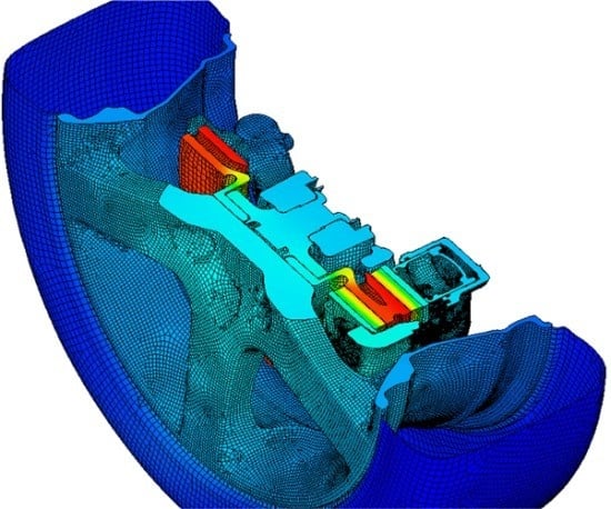
A typical thermal model usually includes all parts that are in immediate proximity to the hot brake disc and participate in the heat dissipation from it: brake disc, brake pads with shims and backplates, calliper with all internal parts, wheel rim and tire, dust shield, wheel hub and knuckle. A typical mesh for the model will contain 3 to 5 million cells. An example is given in
Figure 3.
As mentioned previously, the main task of the thermal solver is to calculate conduction and radiation heat fluxes, combine them with the convective data obtained from the aerodynamic solver and advance in time, calculating new temperature distributions inside the parts modelled.
4.1. Conduction Modelling
Depending on the brake test that is being modelled and the vehicle setup, the brake disc temperature can reach up to 500–700 °C or higher. Other parts, even though reaching lower temperatures, are still subjected to significant spatial and temporal temperature gradients, and as a result, their material properties are going to be affected. Hence, to model thermal conduction within parts, it is of high importance to obtain temperature dependent properties, mainly specific heat and thermal conductivity, for all parts participating in the heat dissipation, or at least for the brake disc and brake pads. These properties can also often be anisotropic, especially for the pads.
The conduction between parts in typically handled by thermal interfaces or thermal links. Two surfaces in contact always have a certain amount of thermal contact resistance. This resistance depends on many parameters, including material properties, surface roughness, and the contact pressure [
20], which can change substantially even depending on the position of tightening bolts [
10]. In the simulation, the contact resistance can be added to thermal links or modelled by adding virtual layers of material between components. It can also be used to replace thin parts that would require too fine meshing otherwise, for example, brake pad shims. However, the assumed values to be used for contact resistance are quite difficult to estimate as there are many variables that must be considered [
21].
One area that requires particular attention is the contact between the piston and calliper body where they are separated by a thin brake fluid film.
4.2. Radiation Modelling
One of the easiest approaches to model radiation between parts is to use surface-to-surface radiation model. This model requires emissivity coefficients being assigned for every surface participating in the heat transfer process. These coefficients can be measured (e.g., using reflectometer) or estimated most of the times, but for some of the surfaces, it can be a challenging task.
The brake disc is a part that is mostly affected by the radiation heat transfer as it is subjected to the highest temperatures. Therefore, the authors have measured emissivity of a large variety of brake discs (all made of similar cast iron alloy material), new and used, and found that the emissivity coefficients can vary between 0.15 to 0.9 depending on the disc surface conditions. This finding is also supported by other investigations available in literature [
10,
22]. Furthermore, operating brake disc would have different emissivity values compared to one that is standing still. This is due to the fact that the emissivity values are temperature dependent and also because there is usually an oxidation layer at the surfaces of the brake that is being cleaned away by the brake pads as soon as the brakes are applied while the vehicle is moving [
23].
As the mesh of the brake disc is often modelled stationary in a thermal model even during driving scenarios, an extra step is required to account for the rotation and avoid local hot and cold spots formation on the disc surfaces. The radiation patches on each of the two sides of the brake disc should be combined to work as a single source/receiver of radiation.
4.3. Brake Fluid Modelling
There are several approaches to model the brake fluid and the selection between them would depend on the importance of the brake fluid simulation for a particular test scenario that is being simulated.
The first and the simplest method is to use a single concentrated mass node representing brake fluid inside the calliper. In this case, thermal links need to be set up in between this node and the corresponding surfaces of the piston and calliper. This method implies that the entire brake fluid volume has the same temperature.
The second approach is to have the brake fluid volume wrapped and meshed so that the brake fluid can be simulated as a solid body with fluid material properties. This method is much more accurate, but as the mixing of the fluid due to convection is not allowed, it can result in rather high temperature gradients inside the fluid; see
Figure 4. Consequently, one should pay attention to the position of the measurement sensor during the experiment and its equivalent in the simulation.
Another option is to try simulating brake fluid as fluid together with the brake lines, but that would increase the computational cost of such simulations even more.
4.4. Energy Input and Disc-to-Pads Contact
Measuring the amount of energy that goes into the brakes and its distribution between inboard and outboard sides of the disc are rather hard issues that are going to be discussed in the Testing section. From the simulation side, it is possible to address this problem using finite element method (FEM) approach [
24,
25]. However, not to increase the complexity of the simulations, the amount of thermal energy added to the system can be estimated. Yet, even the application of this energy inside the thermal model may be a challenging task.
One of the approaches to add energy to the brake system is to apply volumetric heat flux to the circular area of the disc that passes under the brake pads. At the same time, in real life, the energy is generated by friction in the contact pair between the brake disc and brake pads. The energy is then distributed between the contacting surfaces. Therefore, the volumetric flux approach may lead to overprediction of the disc temperatures and incorrect energy flows for the contacts between the brake disc and brake pads.
An alternative approach is to use virtual thermal nodes in between the brake disc and the brake pad surfaces that go in contact when the brakes are applied.
Figure 5 shows an example of how this type of surfaces can be defined. The energy is then “added” directly to the virtual node, allowing to have heat fluxes, that go into the brake pads and the brake disc, changing over time based on the material properties and temperatures of the corresponding parts as they would in reality.
If the simulated test involves stages of driving without braking or soaking phases, the thermal links between the disc and the pads must be adjusted accordingly.
5. Testing
The numerical models and methods developed for replicating any physical test need to be validated against real life experimental data. Therefore, it is important to know and understand the limitations and possible issues with the experimental testing. This chapter covers some of the vital testing issues that are difficult to predict or incorporate into numerical models.
5.1. Typical Test Scenarios and On-Road Testing
One of the easiest ways to test brake cooling performance is to do it on a component level, for example, using brake dynamometer for reduced brake assembly. Unfortunately, component tests, even with partial vehicle geometry [
11], do not represent the on-road driving as there are many uncertainties that must be accounted for one way or the other.
Two typical full-scale on-road vehicle tests scenarios validating brake cooling performance are: mountain descent (also known as alpine descent) and the “Auto Motor und Sport” (AMS) test. Mountain descent test, as the name implies, is conducted on mountains and includes two phases:
Heat-up phase: low speed down-hill driving with constantly engaged brakes on a slope of around 10%;
Thermal soaking phase: the vehicle stands still, and the heat from the brakes is transferred into the brake system and the environment.
AMS test consists of 10 repeated cycles of accelerating up to 130 km/h and braking from 130 to 0 km/h on a flat surface that are sometimes followed by the cool-down phase with constant speed driving or standing still.
Any of the on-road tests will inevitably suffer from the lack of repeatability due to unpredictable and uncontrollable environment. The main considerations are the following:
Air temperature and humidity variations: outside air conditions are changing every day; moreover, considering mountain descent, these conditions can be significantly different at the top and the bottom of the mountain, which in some cases could be compensated by proper monitoring of the driving conditions and calibration of potential numerical factors;
Wind conditions: wind speed and direction change all the time. Considering the cases of low speed driving and especially soaking phase when the vehicle is standing still, the presence of wind can significantly affect the cooling performance of the brake system;
Initial part temperature variations: quite often, several tests are conducted one after another to test various brake and wheel specifications or counteract repeatability issues. Unfortunately, it is almost impossible to get the vehicle into the same exact initial state as it was in before the first run;
Road variations and driver behaviours: none of the roads or drivers are the same, and even if driving the same road with the same driver there will be variations in how the vehicle behaves and what forces it is subjected to. The usage of a driving robot may remove driver behaviour from the equation, but even there, the road will never be exactly the same and neither will the weather conditions.
A lot of these variations can be removed if the tests are simplified and ran in a more controlled environment, but it also means that some of the important variables can be lost. Another approach to tackle repeatability issues is to use statistical analysis; however, testing is expensive and repeating a test 100 times may not be an option.
Other important considerations for matching the simulations and on-road testing are the fan control strategies and the vehicle body movement during various parts of the tests. The first has already been discussed, as for the body movement, when driving downhill, the weight distribution of the vehicle is shifted forwards affecting ground clearance and, hence, affecting the flow inside the wheelhouses. Addition of the braking only increases this effect. Moreover, even on the flat road, inertial radial expansion of tires and aerodynamic lift forces would significantly increase the ground clearance of the vehicle [
26,
27]. Furthermore, the magnitude of this effect depends on the vehicle velocity, which can be of high importance for the AMS tests.
5.2. Wind Tunnel Testing
One of the ways to reduce uncertainties is to conduct tests in a controlled environment. The best option available is to do it in the wind tunnel. This does not only allow choosing the vehicle and wind velocity precisely but also permits to have much better instrumentation as the vehicle is fixed in its position.
Many modern wind tunnels are equipped with various moving ground systems that exist to prevent the formation of the boundary layer and to simulate the ground movement under the vehicle. Unfortunately, wheel drive units are often not powerful enough to withstand the high torque required to replicate braking scenarios. Therefore, braking tests need to be conducted without ground simulation with only the wheel rotating on the dynamometer, see
Figure 6. In the example given, a dynamometer part of the wind tunnel test section has a stationary floor, the rear wheels are standing still, and some additional pipes are present to remove the exhaust gasses. All these modifications are providing extra uncertainties as they alter the airflow compared to on-road conditions.
When imitating mountain descent test in the wind tunnel, constant braking force has to be maintained. Unfortunately, increasing temperatures of the brake pads and the brake discs alter the friction coefficient between these parts; hence, the pressure in the braking system must be constantly adjusted.
Most of the full-scale wind tunnels have a closed loop setup, which means that the air continues to move inside in a circular motion, and it is impossible to bring the air speed to full stop immediately. Consequently, in order to imitate a vehicle stopping at the beginning of the soaking phase, a wind shield can be used to protect the front of the vehicle.
5.3. Sensors and Measurements
Thermocouples are widely used in industry to measure local component temperatures. They are cheap, easy to mount, accurate, and reliable. There are two types of thermocouples: embedded thermocouple and rubbing (also called sliding) thermocouple. In general, thermocouples are wired to measuring equipment, which records the voltage produced and maps the results to calibrated temperatures. Wireless thermocouples can also be used, but they are less reliable due to possible loss of connection and not convenient because of the added weight and space taken by the wireless unit. However, they allow measuring temperature on rotating parts easily.
Thermal cameras can be used in laboratory, but they have the emissivity issue: the temperature measurement needs to be compensated at high values due to the change of emissivity, which as for today, cannot be dynamically modified while recording. Moreover, the thermal cameras cannot be used for brake disc temperature measurements as the wheel rim blocks the view. Furthermore, thermal cameras are very expensive (for the wide temperature ranges observed at braking), bulky, and fragile.
The usual approach is to embed one thermocouple 2 mm below the outer brake pad friction surface, i.e., the brake pad, which is closer to the wheel rim. The thermocouple is inserted from the backplate, making sure that the piston or calliper finger will not put pressure on the wire, which could damage it or in the worst case, cut it. Embedding the thermocouple at the friction surface can destroy it since embedded thermocouples are not meant to be subjected to friction. Also, when inserting the thermocouple, the hole can go through or stop 2 mm before the friction surface, so that the thermocouple is not exposed to frictional debris.
When brake disc temperatures are recorded in some of the experiments, rubbing thermocouples are often used to measure the average surface temperature on a certain radius at the contact patch. Also, pyrometers can be used for the same result. Alternatively, the brake disc can also be drilled with thermocouples embedded under its surface. This setup would require a slip ring connector on the outside of the wheel to transfer the signal from the rotating disc, similar to the one in
Figure 6.
When the brake fluid temperature needs to be measured, a special thermocouple embedded in the brake calliper bleeding screw is normally used; see
Figure 7. This is not where the brake fluid reaches its highest temperature, but this is the only location that is safe enough to measure the temperature without affecting the strength of the calliper. Brake fluid temperature, as provided by the experiment, will be a single point measurement, while as it was mentioned earlier in
Section 4.3, CAE simulations allow seeing the brake fluid temperature gradient.
Capturing spatial temperature gradients of the brake fluid experimentally is hardly possible, and even for the parts that are easier to access, there is always a limit of how many thermocouples can be used. Any additional thermocouples do not only increase the time required for test preparation but also alter the airflow around parts.
5.4. Disc Deformations and Hot-Spotting
Most of the parts will experience thermal expansion when subjected to high temperatures. For the brake cooling tests, the most important deformations happen to the disc as it experiences highest temperature changes. Unfortunately, thermal expansion is not the only deformation that occurs during braking. Conning is the type of deformation that occurs when the brake disc deforms elastically and/or plastically at the neck due to cyclic cooling and heating. Another important effect is hot-spotting.
Hot-spotting is related to a phenomenon called Thermo-Elastic Instabilities (TEI) [
28]. When braking, the pair of brake pads is pushed towards the brake disc, which, in return, generates frictional heat flux at the sliding interface, which is proportional to the contact pressure. Therefore, if some uneven pressure distribution arises at the friction surface, the areas where the pressure is higher experience a higher temperature increase. This, in turn, causes greater local thermal expansion and, thereby, leads to further local pressure increase [
29]. Hot-spot positions change with every new load cycle; therefore, measuring the disc temperatures with embedded thermocouples can have serious repeatability issues even when testing in the wind tunnel.
Any uneven pressure distribution at the contact between the brake disc and brake pads leads to uneven deformations and, consequently, non-uniform heat fluxes at the contact interface. These effects are typically unaccounted for in the brake cooling simulations but should be kept in mind when comparing the results between real and virtual models.
5.5. Energy Input Estimation
Temperatures in the brake system are directly affected by the amount of energy that goes into contact between the brake disc brake and pads. However, estimating this amount for each pad-to-disc contact is not a trivial task.
When the vehicle brakes, one can have a good estimation of changes in kinetic and potential energies. Unfortunately, not all of this energy goes into the braking system. Some of it is spent on overcoming rolling and aerodynamic resistance and some ends up in drivetrain and other losses. Moreover, depending on the vehicle weight distribution and brake system setup, front and rear brakes would have an uneven split between them. Typically, front brakes take most of the load due to higher vertical force on front wheels and vehicle stability reasons. Additionally, since the vehicles are not symmetrical, brakes on the left and right side of the vehicle may have slightly different temperatures, which would lead to changing friction and different energy input for them. The same principle applies to inboard and outboard sides of the brake disc where the energy input would differ. Furthermore, the ratios in these splits would change during the braking test cycle, making it almost impossible to estimate them exactly at any given moment.
During the tests in the wind tunnel, the amount of energy added to the braking system is easier to estimate as the braking force is recorded by the dynamometer. Nevertheless, the amount of losses in various system parts and the distribution between two contact surfaces of the disc are still unclear.
6. Concluding Remarks
Brake cooling performance evaluation is important since it allows safe vehicle operation in even the most extreme circumstances. Currently, most of this evaluation is performed using expensive experimental testing methods; however, there is extensive ongoing work to replicate such testing using CAE simulations. In this paper, some important effects, findings, and issues needed to be considered during this process were summarized.
Brake cooling CAE simulations are complex since a large amount of material data and other properties are missing or even impossible to estimate. Additionally, there are several simulation approaches, all having different advantages and disadvantages, and a common denominator that they all require considerable simplifications.
Nevertheless, it has been shown that CAE simulations give satisfactory results, especially when comparing different design choices. The simulations are not only cheaper but can also be performed at earlier stages of the vehicle development process, even when there are no prototypes available. Furthermore, as the simulations have perfect control over used boundary conditions, they provide perfect repeatability, which is something that the experimental testing is certainly struggling with. In addition, virtual models give important physical insights into the complicated heat dissipation process. The CAE simulations provide not only the temperature gradients within parts, but also the heat flux distributions for convection, conduction, and radiation for every part surface or part contact at any given time. For instance, experimentally determined brake fluid temperature is measured in a single point, while CAE simulations offer spatial temperature gradients inside the calliper.
At this time, it is not yet possible to replace the experimental testing with simulations, but two approaches can be used together to complement each other. Moreover, as the computational resources become more affordable, the amount of virtual testing will increase. However, much more work is still needed to improve the existing methods and develop new ones before they can completely replace the physical testing.


