Long-Term Monitoring of Sensible Thermal Storage in an Extremely Cold Region

Abstract

We present more than one-year of monitoring results from a thermal energy storage system located in a very cold place with a long winter season. The studied house is in Palmer city, Alaska (~62° N, ~149° W). The house is equipped with solar PV for electricity production and solar thermal collectors which were linked to a sensible thermal energy storage system which is underneath the house’s normally unoccupied garage and storage space. Sensors were installed in the thermal storage and solar thermal collector array to monitor system temperatures. In addition, TRNSYS was used for numerical simulation and the results were compared to experimental ones. The maximum observed garage ambient temperature was ~28 °C while the simulated maximum ambient garage temperature was found to be ~22 °C. Results indicate that seasonal solar thermal storages are viable options for reducing the cost of energy in a region with extended freezing periods. This is significant for Alaska where the cost of energy is 3–5 times the national average.

1. Introduction

Climate change and global warming have led to increased focus on renewable energies research in increasing reliability and capacities of solar thermal energy systems. Active and passive solar types of solar thermal storages have been researched extensively for applications in moderate temperature zones. Research in application of solar thermal storage in colder regions such as Alaska is scarce. According to the ASHRAE (American Society of Heating, Refrigerating and Air-Conditioning Engineers) Applications Handbook, active solar thermal systems aren’t appropriate in regions with extended duration of very cold temperatures [1]. In the guidance provided in the ASHRAE handbooks, the storage medium has almost always been assumed to be water, and when rocks are applied for the storage, air is used to transfer heat [2]. Water, as a heat transfer medium, is more desirable than air because it has a high specific heat. However, big water storage tanks lead to high initial and maintenance costs. For large scale applications, rock beds and sand-beds have proven to be economically feasible at $5-$20US per ton. Although sand-beds have 20%–40% more specific heat than that of water, they have attracted researchers’ attentions because of their low cost.

In a rock-bed system, the main thermal storage medium is rock. Some of the forms of these types of storage medium are packed rock-bed, sand, bricks and small pebbles. In comparison to other methods of thermal storages, the rock-bed thermal storage systems offer several attractive advantages. In these systems heat is transferred via air requiring no piping systems as compared to water thermal storage systems. In addition, they do not require expensive drilling work.

On the other hand, because of low specific heat, rock-bed thermal storages require large amounts of material to be used. A rock-based system needs to have at least 3 times more volume than a water-based system to provide the same amount of energy. A compromise approach to avoid an expensive initial capital cost of a water tank system and make up for the low energy (with low initial cost) of a rock-bed system is the use of a hybrid gravel/water thermal storage system.

Dry sand-bed thermal storage systems can reach high temperatures, thus providing better energy quality. This is particularly vital for systems applied at commercial scale. In addition, they provide the flexibility to be easily incorporated into the design of the existing facilities grounds or structures, such as the parking lot. However, there are challenges in determining accurately thermal properties of sand and sand like substances due to the varying compaction rate and moisture content.

As far as thermal collectors are concerned, residential solar thermal has been done almost exclusively with evacuated tube or flat plate solar thermal collectors. Flat plate solar thermal collectors have a higher thermal efficiency but tend to be limited by the boiling temperature of water for their maximum temperature. Additionally, flat plate collectors are prone to efficiency losses due to the reflection of light off the surface when the incident angle is not perpendicular to the collector. This reduction in efficiency due to the incident angle is referred to as the incident angle modifier (IAM). While the IAM on flat plate collectors can be readily determined, it is more difficult to determine for evacuated tubes due to the cylindrical shape of the tube and variety of shapes the absorber can come in and the specificity of an individual location. Kalogirou indicated that evacuated tube solar collectors were preferred for cold climates due to the inherent freeze protection of the intermediate fluid and the significantly reduced thermal losses to the environment when compared to flat plate collectors [3].

An area of some success has been in utilizing solar thermal systems in normally unoccupied parts of a building and power plants. M.K. Ghosal et al. [4] used solar thermal energy storage systems for greenhouse applications that significantly enhanced the thermal performance of the building as compared to traditional heating systems. Another area of application is that of Concentrated Solar Power (CSP) thermal storage. CSP have been shown to have great potential in offsetting the diurnal nature of solar availability. It’s been reported that rock-bed filled with high temperature oil could be utilized for storing a significant quantity of heat for CSP systems [5].

Over the past 35 years researchers have focused on developing effective and efficient ways storing thermal energy [6,7]. For example, in Germany, the first long-term thermal energy storage was built as a research installation in 1984 [7]. In Germany, The first large-scale seasonal solar thermal energy storage (STES) was built in Hamburg in 1996 [8]. This STES consisted of a 4500 m³ concrete tank buried underground. It was charged by 3000 m² (2.1 MW) of solar collectors and delivered heat for space heating and domestic hot water supply purposes.

Antoniadisa and Martinopoulosa [9] numerically studied the performance of solar thermal energy storage for residential application in Thessaloniki, Greece. They found that the system can cover 52.3% of the heating load for typical residential building in this region. Ghaebi et al. [10] studied a confined aquifer under different configurations for cooling and heating of a residential complex located in Tehran, Iran. Their results of parametric studies, using ANSYS FLUNET, showed that coupling a heat pump to the thermal energy storage for both cooling and heating of the buildings yielded the best result, with a COP of 17.2 for the cooling, and a COP of 5 for the heating. A passive solar system was installed for application in countryside Thailand, in a region without access to utilities [11]. The system heats a rock-bed with opaque surface. Heat is transferred to the living zone by means of natural convection. Although the system is reported to achieve the aim of increasing the temperature of the living space during cold evenings, this increase was beyond the comfort level, with nearly 45 °C. This indicates the need for an active system with proper controls and thermal regulation. Sweet & McLeskey [12] conducted numerical study of an active solar thermal residential building, situated in Richmond, Virginia. The parametric numerical study considered sand-bed thermal storage with varying sizes connected to solar thermal collectors. In almost all cases it took five years for the sand-bed to achieve an equilibrium seasonally and become “fully charged.” They suggested that inappropriate sizing of the thermal storage system would result in insignificant heating. On the other hand, an extremely small system wouldn’t allow for effective storage of heat for seasonal use, and excessively huge systems wouldn’t attain a required temperature to provide adequate heating.

Researchers at Virginia Commonwealth designed a thermal energy storage system made of a sand-bed for a big part of the university [13]. They used a sand-bed insulated with 10 cm all around and connected to flat plate solar thermal collectors. They reported that 91% of the building’s heating requirements could be satisfied by this system. Getu et al. investigated the application seasonal solar thermal storage in cold regions [14,15]. Their short-term monitoring and modeling results indicated the applicability of seasonal solar thermal storages in cold regions. Schlipf et al. [16] investigated influence of sand grain size on the thermal capacity of a thermal storage and found that small grained material (diameters of 2 mm or less) has very good potential as a thermal storage material. This is because temperature is distributed very fast within the material, enabling the thermal energy to enter and leave very rapidly during charging and discharging. Allen et al. conducted experimental study of the particle size and bed length for optimal operation below 100 °C. They reported that particles about 0.02 m in size and 6 m bed lengths provide optimum operation [17].

Seasonal thermal storage systems have been implemented at the community level as well. For example, the solar district heating system combined with borehole thermal energy storage (BTES) in the Drake Landing Solar Community (DLSC) has been reported to provide 97% of the annual space heating demand with solar power [18]. Singh et al. [19] conducted a heat transfer study and friction factor characteristics on a packed bed having different sphericity values, low void fraction and larger size. They found that spherical elements with lowest void fraction had the best the performance. Nems et al. [20] studied ceramic brick packed-bed. They reported that heat storage process in this system has high efficiency, in the range of 74%–96% for the airflow rate of 0.0068 m³/s and 72%–93% for airflow rate of 0.0050 m³/s.

Several researchers have worked in the area of developing methods for assessing the energy-efficiency and cost-effectiveness of exterior walls suitable for cold climate conditions. Baglivo and Congedo [21] developed a method for the analysis of the design of energy-efficient precast walls suitable for cold climates. They reported that it was possible to achieve high performance by thin (18–20 cm) and ultra-thin walls (less than 18 cm). Wang et al. [22] also developed a method of assessing cost-effectiveness of insulated exterior walls for residential buildings in cold climate. The proposed method takes into account the main expenses and profits of using insulated exterior walls during a building lifecycle. They reported that the developed method is useful in evaluating insulated exterior walls easily and properly, enabling designers and government agencies to assess the cost-effectiveness of different walls very quickly.

A literature review indicates that most research on solar thermal storage has been done for commercial and industrial applications. Most residential applications were limited to diurnal solar thermal systems for space heating or domestic hot water production in remote undeveloped areas with entirely passive systems. There is limited research of solar thermal energy storage systems for residential use, especially in cold places like Akaka. In this work, we will provide detailed results of the long-term monitoring of an experimental house with thermal storage. We will also provide detailed method for determining the thermal properties of the thermal storage. Finally, we will compare results of experimental measurements to numerical results.

2. Experimental House

For this study, a 2-story house was built in the city of Palmer, Alaska. Since the house has been described in detail in [14,15], only a brief overview is given here. The house has normally a vacant garage and storage area. The upstairs part of the house consists of living area of 54 m² (581 ft²). The house is designed to be Net Zero Energy (NZE). To achieve NZE status, electricity supplied from the utility grid at times of low solar production and is fed to the utility grid at times of high solar production. The house utilizes non-traditional, high efficiency construction techniques, such as Arctic walls [23]. The design of Arctic walls prohibits a direct thermal path between the inner and outer side of the wall. Furthermore, permeable membrane cellulose which are densely packed are utilized as insulators instead of a traditional vapor barrier [23]. Each face of the house is directed in a true cardinal direction. The PV panels and the evaluated tubes face the south side as shown in Figure 1. Densely packed cellulose is also used for roof insulation. The walls and the roofs have thermal resistance values of RSI-10.6 (US R-60) and RSI-15.9 (US R-90), respectively.

3. Experimental Setup

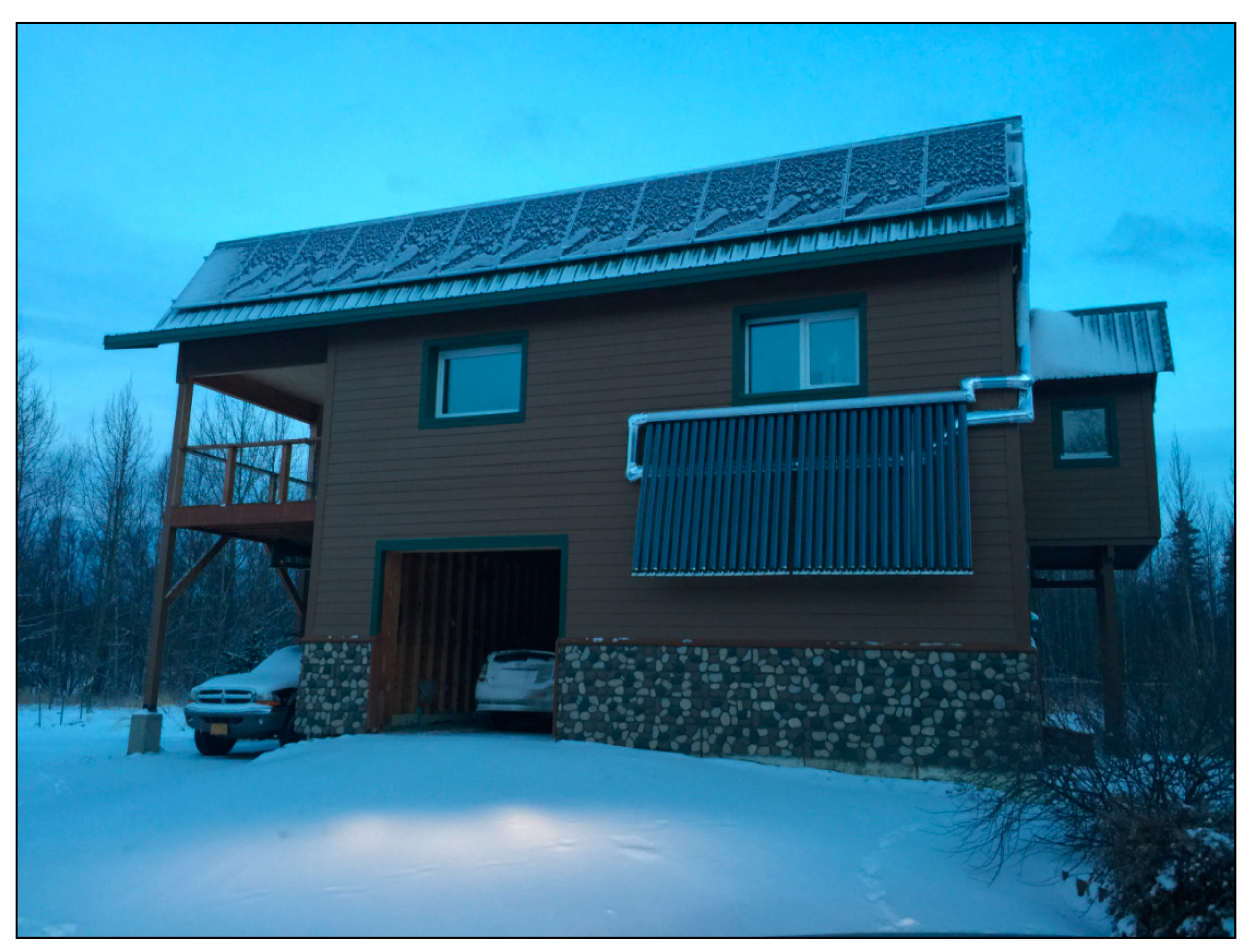
The total rated power of the panels is 3.705 kW (285 watt each). 13 panels were installed at an inclination of 60° on the roof. These Solar PV panels are connected to 5000-watt capacity power inverter and then to the 2-way meter linking to MEA- Matanuska Electric Association, Inc. power grid. Evacuated solar tubes were installed at 75° angle of inclination on the houses’ south facing wall.

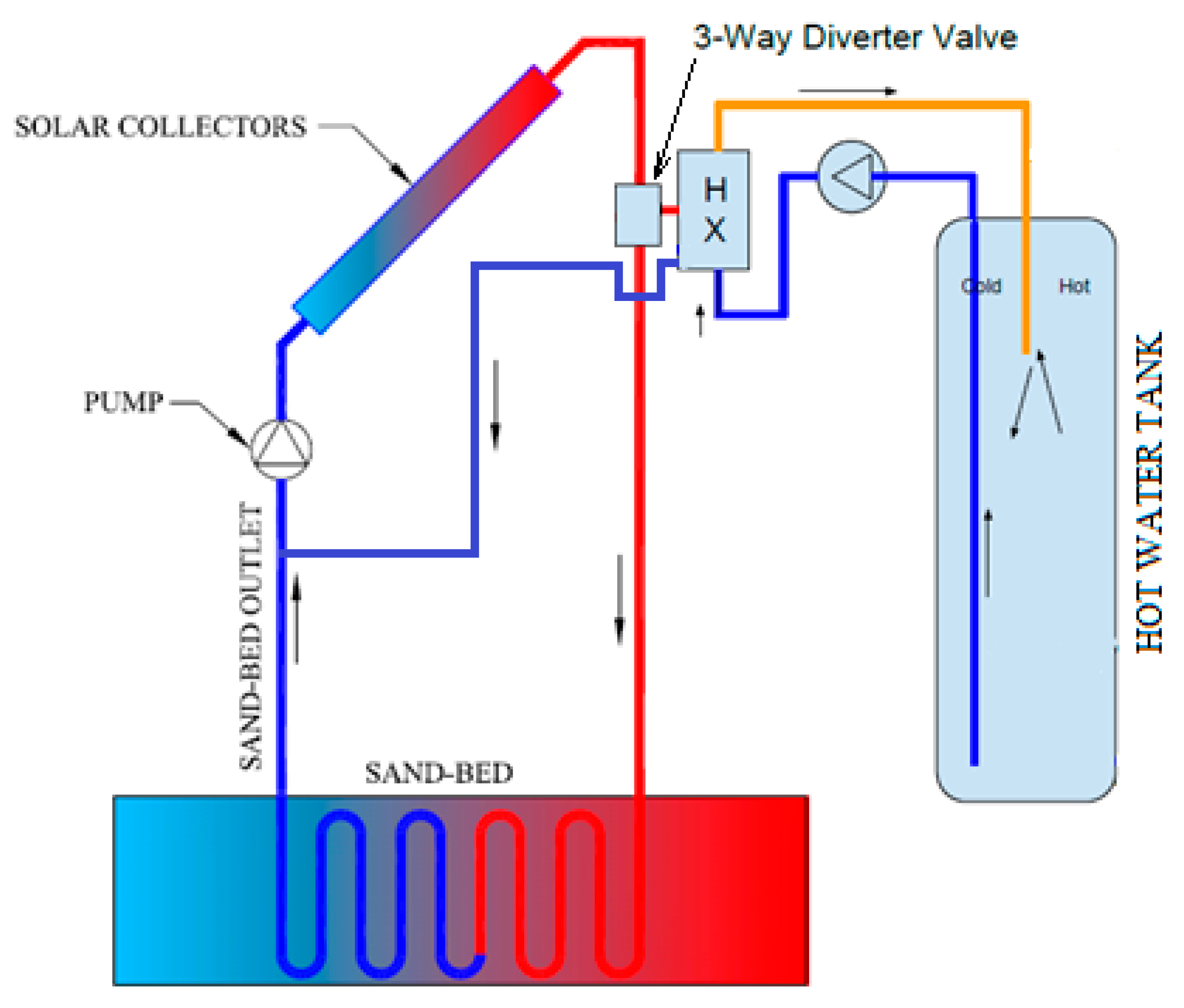
Glycol-water solution is heated by the evacuated tube solar collectors during normal operation and passes through the sand-bed thermal storage that, during normal operation, passes through a heat exchanger to heat the domestic hot water tank. When the domestic hot water tank is not calling for heat, the excess heat is sent to the sand-bed under the garage floor for heating. The installation enables also an alternative mode of operation to produce domestic hot water if needed. In this experiment, though, during the entire period of the experiment, the heat from the solar collectors was used to heat the thermal storage only. The piping system diagram for the setup is show in Figure 2. The solar thermal storage not only acts as a way to claim the normally unusable heat, it also acts as a load shed for the evacuated tube solar thermal system. The need for a load shed was identified as the stagnation temperature of the solar collector was 221.1 °C, which could break down the propylene glycol and possibly create a vapor pocket. Utilizing the thermal storage as a load shed kept continuous flow through the system, preventing the fluid from overheating and breaking down the glycol or creating a vapor pocket.

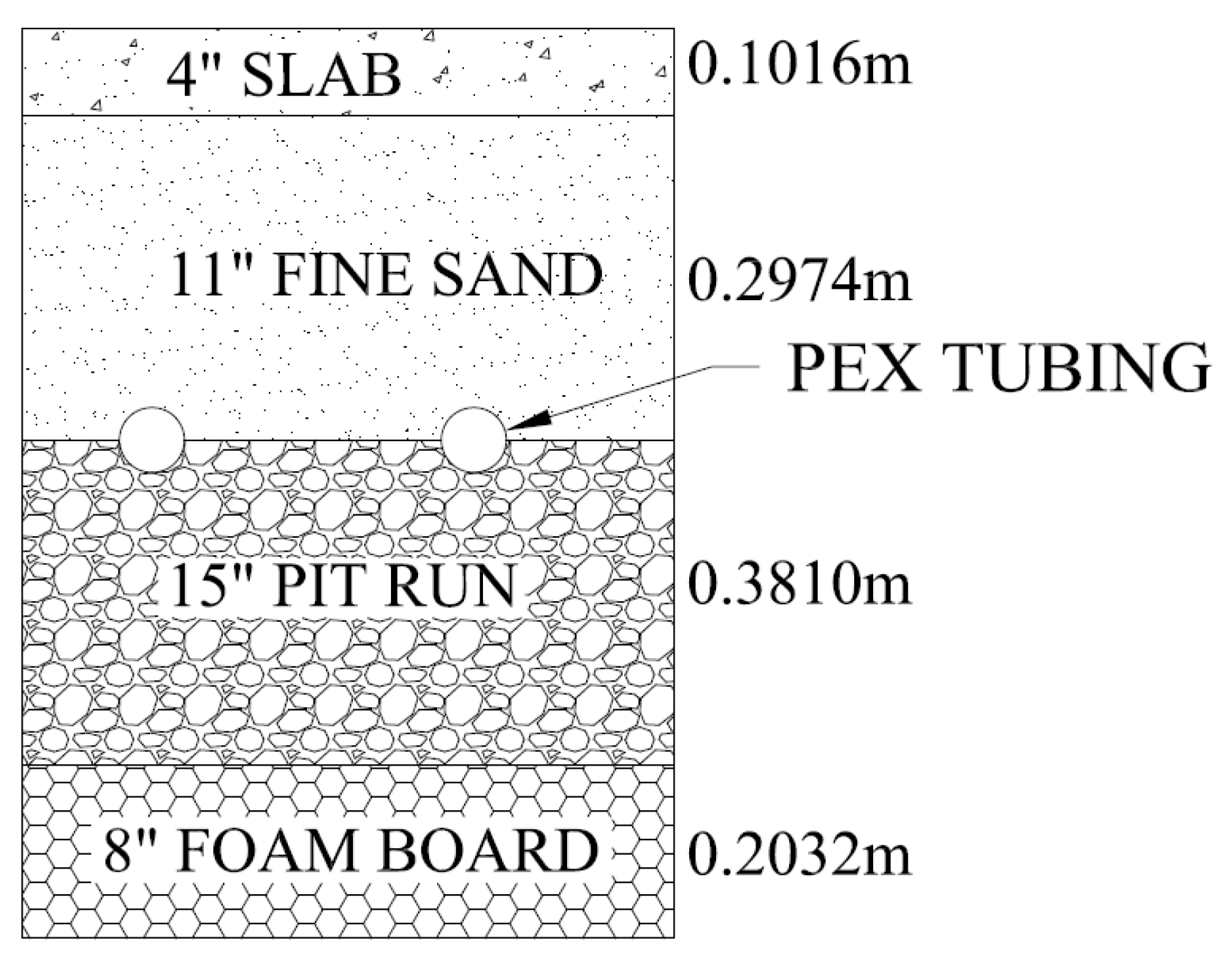
The garage floor consisted of a 6.502 m (21’-4”) by 8.331 m (27’-4”) by 10.2 cm (4”) concrete slab in thickness, with 1 garage door and 1 man-door [15]. Below the 4” thick garage slab was the thermal storage containing approximately 29.7 cm (11”) of fine sand and 38.1 cm (15”) of pit run gravel as shown in the floor cutaway view, Figure 3.

A 20 cm (8”) thick polystyrene foam was used to insulate the thermal storage from the bottom. The thermal resistivity of polystyrene foam was found to be RSI-5.64 (US R-32). A 20 cm (8”) thick polystyrene foam was also used to insulate the four sides of the (8”) of polystyrene foam board on both sides of the poured concrete foundation wall.

Resistive Temperature Detectors (RTDs) and thermocouples were used in measuring temperatures for the experiment. RTDs were embedded into the core of the thermal storage and placed in the glycol-water solution inlet and outlet flow streams. The RTDs were connected to a Caleffi data logger or other Caleffi devices. Thermocouples were also placed in the core and on the surface of the thermal storage, as well as in the thermal storage inlet flow stream. Each thermocouple was connected to an individual Lascar data logger. Flowrate was measured with a rotary pulse meter and connected to a Caleffi data logger. Garage ambient as well as outside ambient temperatures where measured and logged by an all-inclusive Lascar electronics device. The solar thermal controller purchased from Caleffi was designed to work with Pt1000 RTDs. Based on the input requirements of the controller, a total of nine RTDs were placed in the thermal storage, evenly spaced in three layers of three. Additionally, RTDs were put in the thermal storage inlet and outlet flow streams. RTDs used for this research were Caleffi Part Number 257,205, FKP6 collector sensor Pt1000, Caleffi North America Inc., Milwaukee, WI, USA, and had an accuracy of ±0.3 °C from −50 °C up to 100 °C. For 100 °C and over, the accuracy was ±0.8 °C up to the maximum operating temperature of 250 °C.

The solar thermal system controller was a Caleffi iSolar Plus, a commercially available two tank solar thermal controller. A controller, which was configured for a single zone, was used to activate the pump when a temperature difference of 5.778 °C (12 °F) was reached to send fluid from the evacuated tubes to the thermal storage. As mentioned earlier, during the period of this research all heat was directed to the thermal storage. Fluid flow measurements were captured by a Caleffi V40 flow meter, which sends an impulse control signal for every liter of fluid flow that is measured. An impulse flow meter was used to measure thermal storage inlet and outlet flow rates. A data logger (Caleffi DL3) was used to store the measured data.

Data logging of the thermocouples was carried out with Lascar data loggers. The EL-USB-TCs can read type J, K, and T thermocouples with accuracy of ±1 °C and a resolution of 0.5 °C. Outside ambient as well as inside the garage ambient temperature was recorded using Lascar Electronics part number EL-USB-2. The EL-USB-2 had an accuracy of ±0.55 °C and a resolution of 0.5 °C. Both devices enable user selection of data logging interval and reading via USB connection. A software supplied by the Lascar Electronics is used to access the data via USB connection.

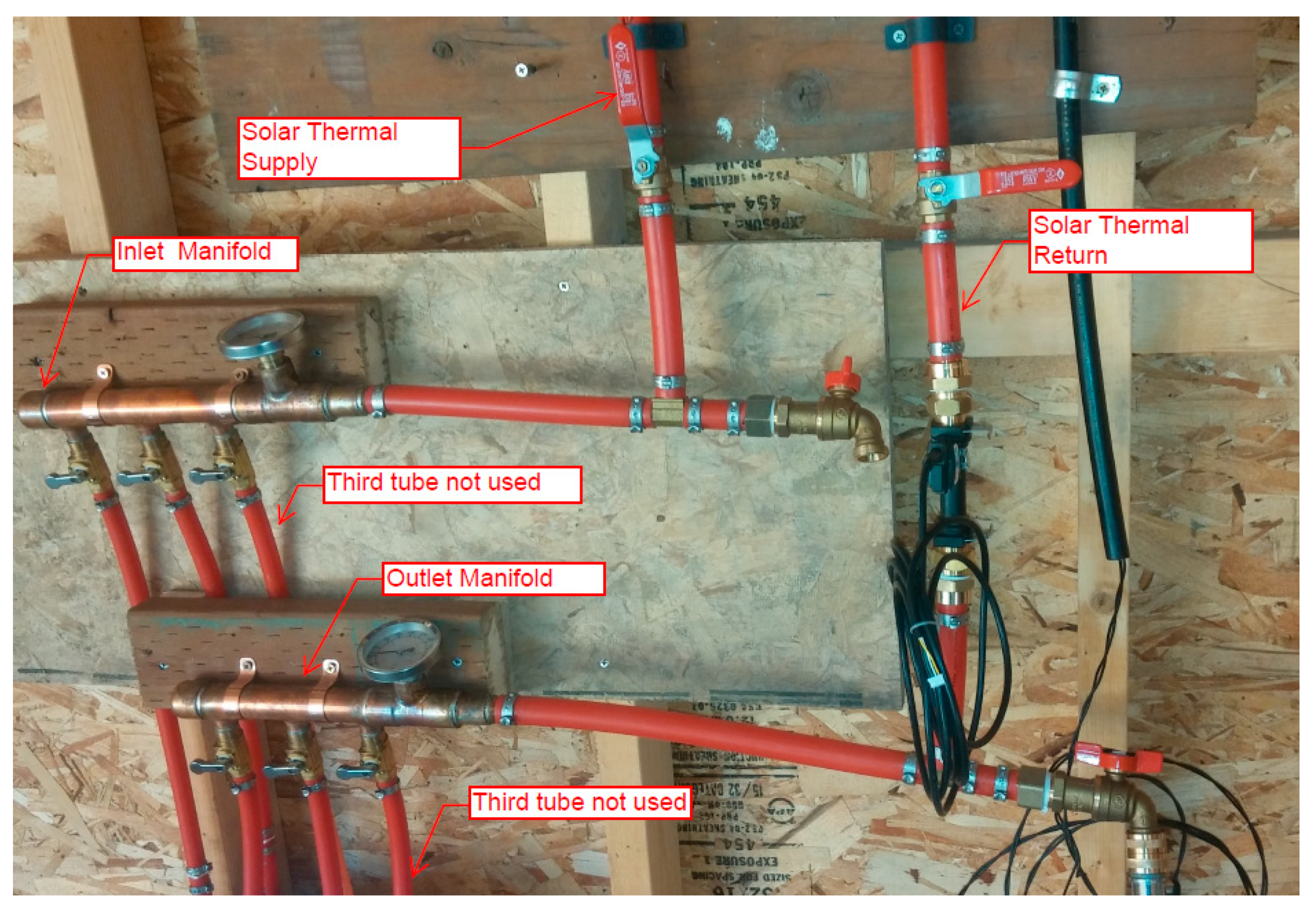
A total of 91.4 m (300 ft) PEX tubing had been installed in 2 loops in the sand-bed [9,10]. The two loops are run to manifolds at the north side of the garage where they were tied into the solar thermal inlet and outlet, as shown in Figure 4.

The supply and return tubes then run upstairs to the controller and flow pump (and domestic hot water), which was not used for this experiment where it continued to the solar thermal array on the exterior of the home’s wall. A number of thermocouples and RTDs were embedded in the thermal storage to map the temperature distribution inside the thermal storage [14,15].

Data loggers actively recorded the thermal storage thermocouple readings on 15-min intervals and glycol-water mixture RTD and thermocouple readings on 1-min intervals. Due to the limited number of data points capable of being stored by an individual data logger, the data was retrieved on a weekly to bi-weekly basis, after which the data logger was reset.

4. Determination of Thermal Storage Thermal Properties

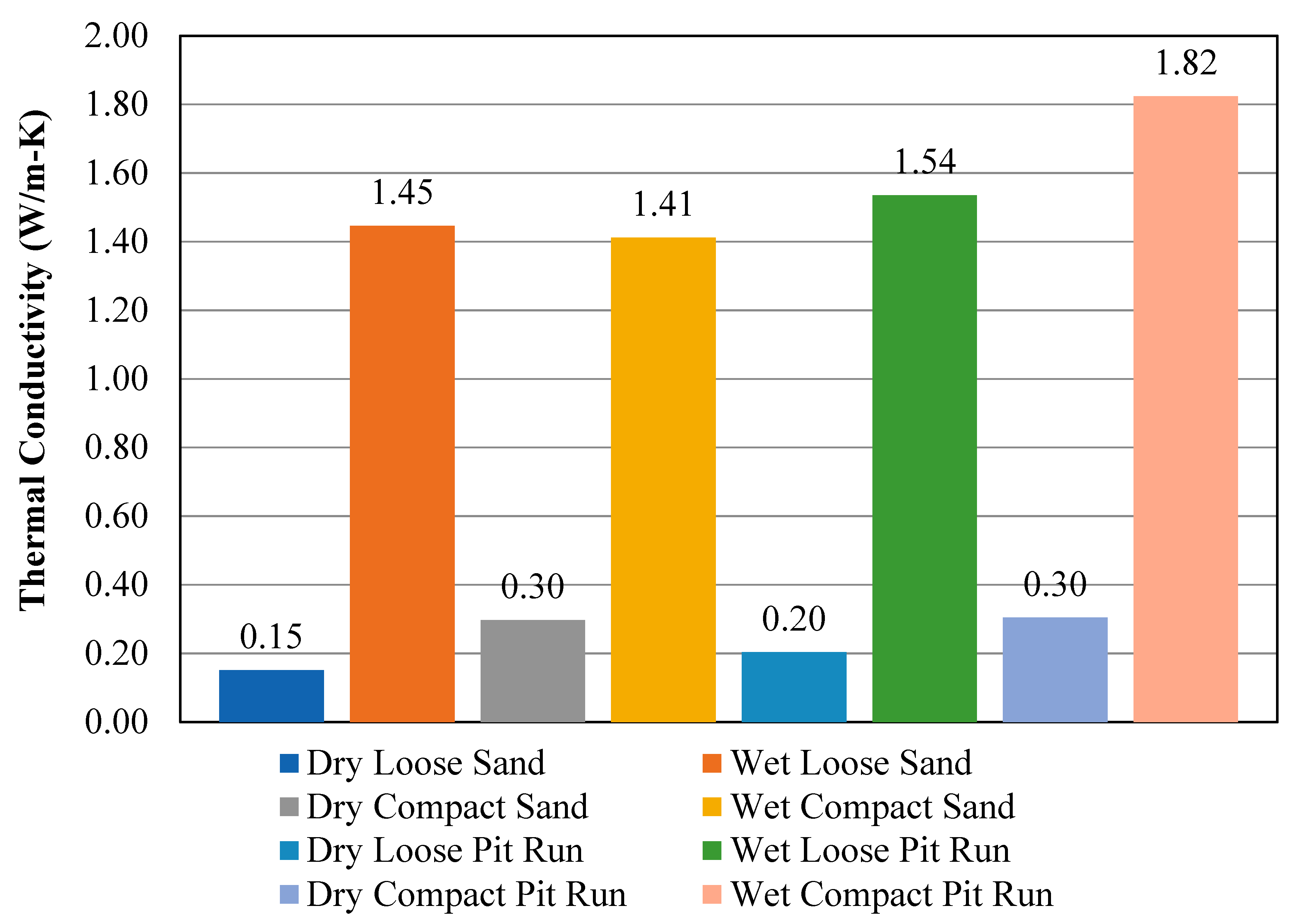
As mentioned earlier, the thermal storage is composed of pit run, fine sand and concrete of which the thermal properties needed determination. A sample of the fine sand was taken from the site from an excess material pile. Specific heat and thermal conductivity properties were determined using KD2 Pro Thermal Properties Analyzer. As reported by M. Golob [24] thermal properties are difficult to determine and vary dramatically with the moisture content and compaction rate. Soil thermal conductivity is the most sensitive parameter in terms of STES system performance [25].

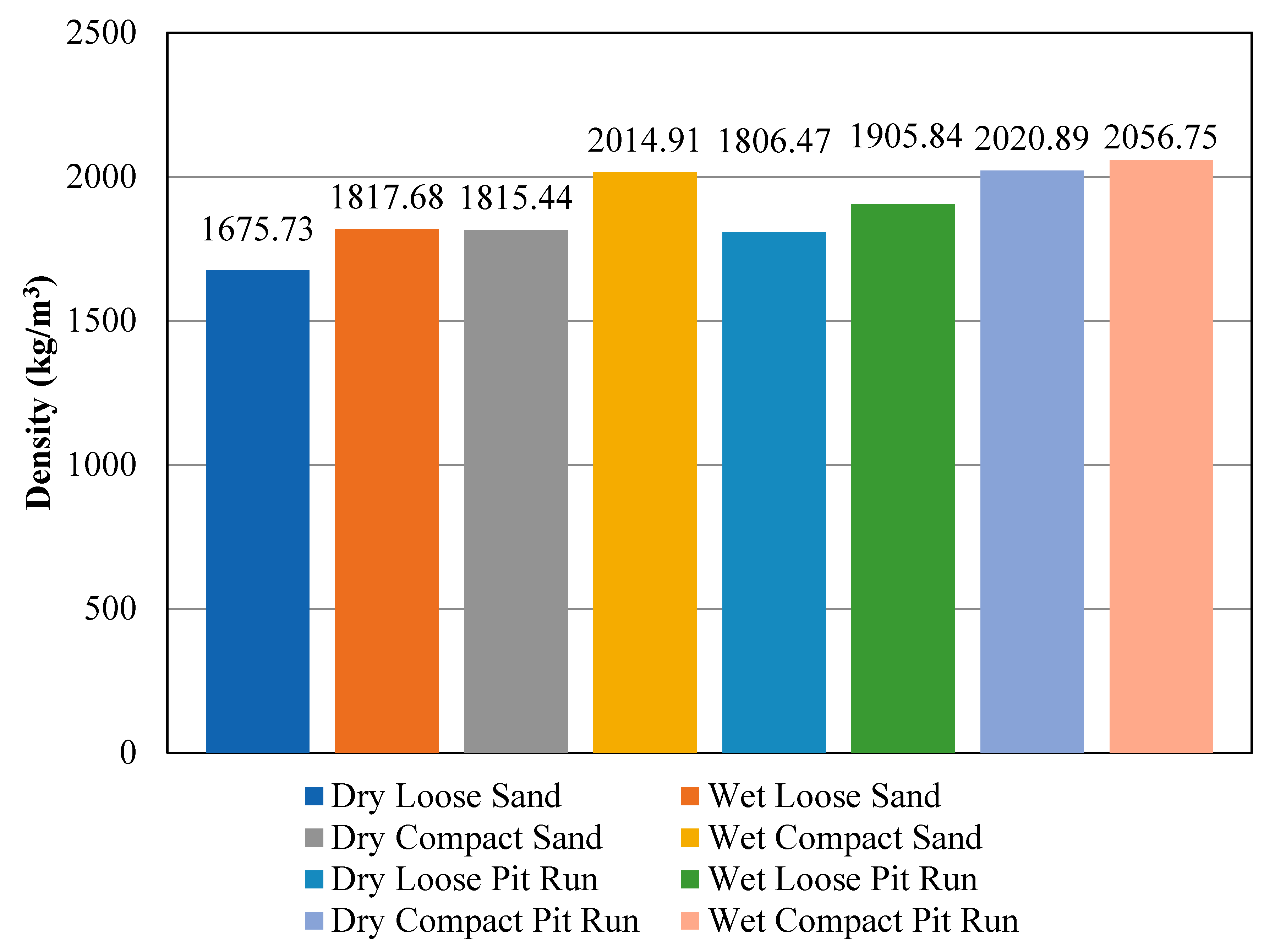
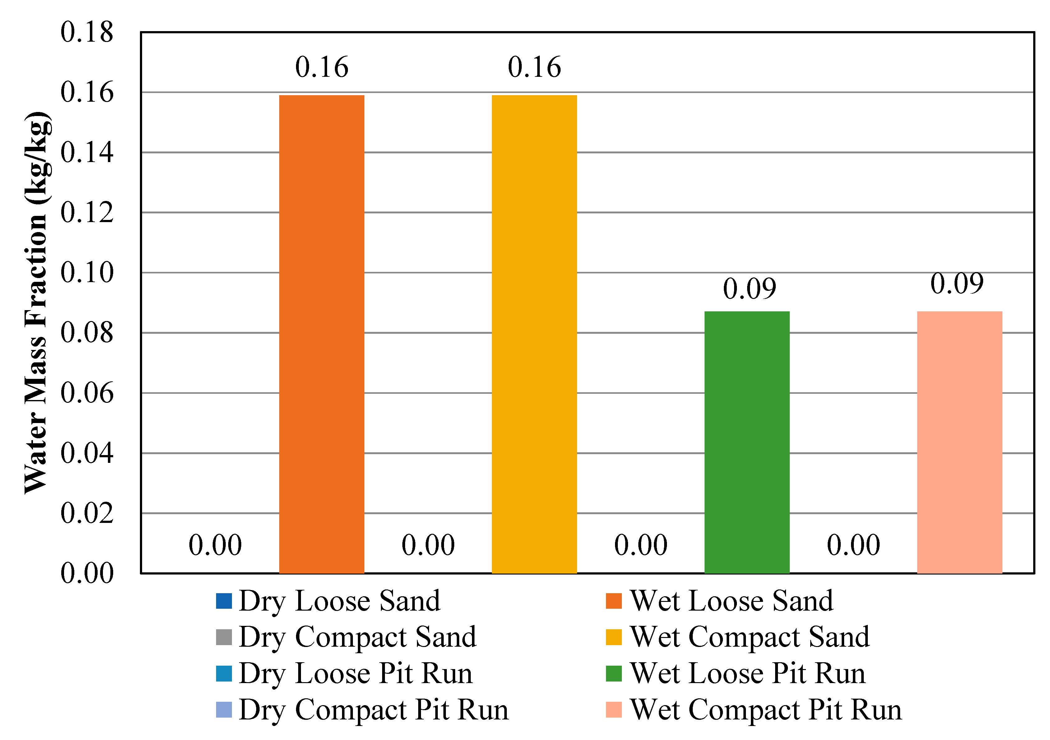
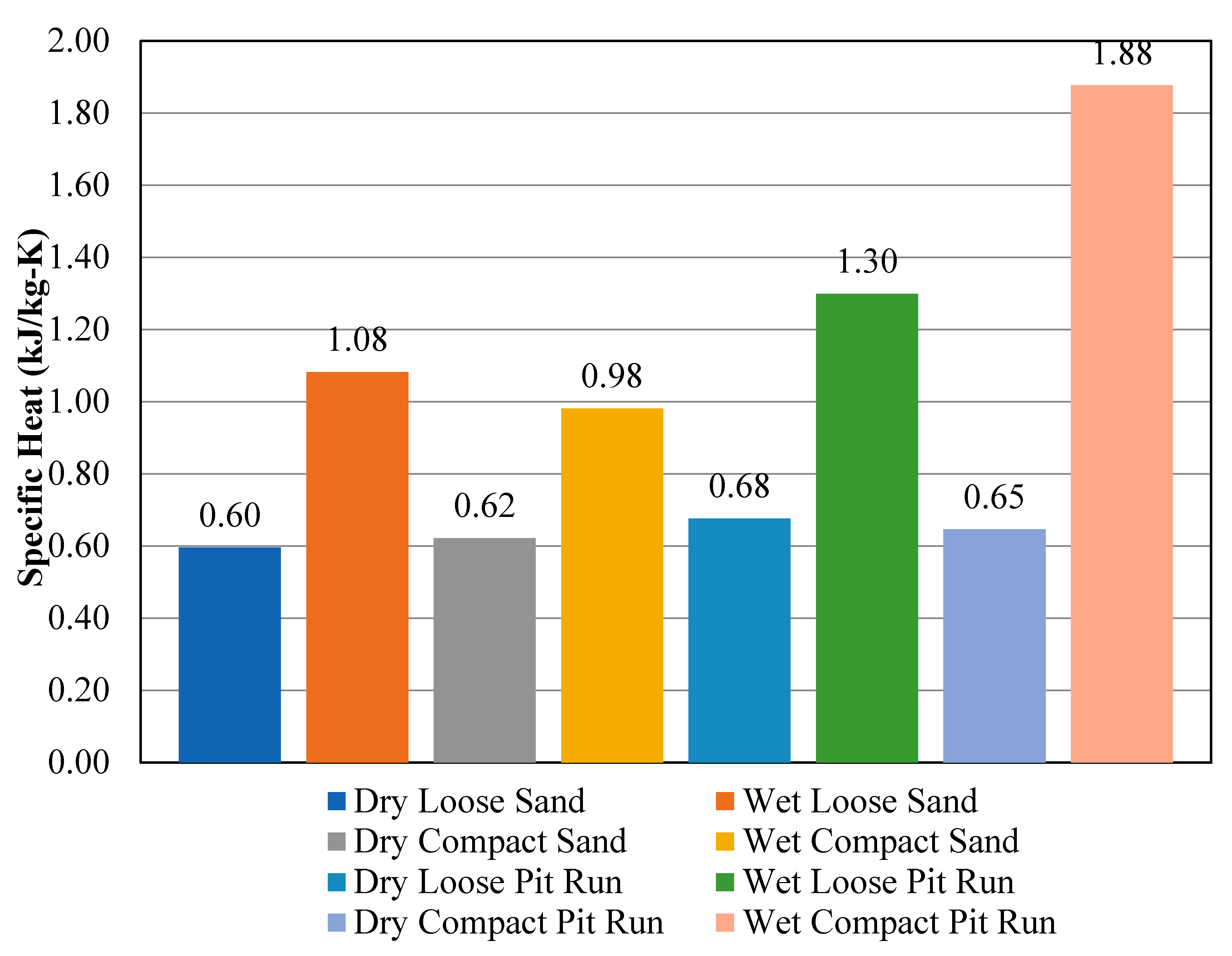
Therefore, both the sand and pit run samples were evaluated at two compaction and moisture content ratios. The sand and pit run were compacted manually with the sand being compacted as adequate for pouring the concrete garage floor. Thermal properties were determined for wet, dry, loose and compact conditions. The determined properties are shown in Figure 5, Figure 6, Figure 7 and Figure 8.

The specific heat of all types of samples (dry, wet, loose, compact and a combination of these) was obtained. All dry samples had specific heat within 14% to 16% that of water. All samples showed significant improvement in their specific heats after the addition of water. Sand which was compacted had the lowest heat at 23%. Pit run which was compacted had the highest heat at 45% water. Sand showed a higher ability of holding water. However, it was the pit run which had the greater specific heat. Using Equation (1), the thermal properties of samples were calculated to obtain a single specific heat for different moisture content and level of compaction along with the constant concrete thermal properties. Results of the combined specific heat for the fine sand and the pit run are provided in

Table 1. Combined sand and pit run thermal properties [9].

Thermal Storage (Sand and Pit Run) Properties
Loose, Dry		Unit
Thermal Conductivity (κ)	0.34	Wm−1 K−1
Specific Heat (Cp)	0.67	kJ kg−1 K−1
Density (ρ)	1824.3	Kg m−3
Total Mass (m)	75,301.7	kg
Compact, Dry
κ	0.45	Wm−1 K−1
Cp	0.67	kJ kg−1 K−1
ρ	1982.8	Kg m−3
m	81,841.2	kg
Loose, Wet
κ	1.48	Wm−1 K−1
Cp	1.16	kJ kg−1 K−1
ρ	1926.1	Kg m−3
m	79501	kg
Compact, wet
κ	1.62	Wm−1 K−1
Cp	1.42	kJ kg−1 K−1
ρ	2073.8	Kg m−3
m	85,600	kg

.

The concrete thermal properties were estimated using tabulated data with a thermal conductivity of 1.4 Wm⁻¹ K⁻¹ and specific heat of 0.88 kJ kg⁻¹ K⁻¹ [26]. The combined specific heat for the thermal storage was determined using the sum of the products of each material’s specific heat to the material’s volume ratio of entire sand pit, as shown in Equation (1).

$$C_r=\frac{V_{concrete}}{V_{total}}{C}_{concrete}+\frac{V_{sand}}{V_{total}}{C}_{sand}+\frac{V_{pitr run}}{V_{total}}{C}_{put run}$$

(1)

where C is specific heat and V is volume.

During numerical simulation, thermal conductivity and specific heat values were adjusted iteratively to obtain results which more accurately fit the measured data.

Table 2. Parameters and input variables of Type 10 rock-bed.

Type 10: Rock Bed Thermal Storage
Parameters		Unit
Cp of air	3.6906	kJ kg−1 K−1
Rock-bed length	0.762	m
Cross-sectional area	54.1715	m2
Perimeter	29.6668	m
Specific heat of rock	0.66848	kJ/kg-K
Apparent rock bed density	2035.3	kg/m3
Loss coefficient	0.6384	Wm−2 K−1
Effective κ	1.6164	Wm−1 K−1
Input		Unit
Temperature into top	−10	C
Flowrate into top	0.1	kg/h
Environment temperature	3.79	C

gives thermal storage data used for TRNSYS simulation.

5. Water-Glycol Mixture Thermal Properties

The thermal working fluid was a propylene glycol-water solution, glycol is added to water to prevent freezing of the lines and potentially rupturing the tubes. Propylene glycol has a lower specific heat than water, the percent glycol was determined using a refractometer and its specific heat interpolated from tabulated data shown in

Table 3. Specific heat of propylene glycol-water mixture [13].

	Percent Glycol by Weight
	100	80	60	40	20	10	0
Specific Heat (J/kg·K)	2458	2876	3328	3768	4061	4124	4186

. A refractometer was used to find glycol percentage in the glycol-water mixture. The mixture contained 43% glycol by volume. The density of glycol was measured to be 1.04 kg/m³, using the density of water at 1 kg/m³, the aggregated density of the solution was therefore found to be 1.017 kg/m³. The specific heat of the glycol-water mixture was then linearly interpolated from Table 3 and found to be 3.691 kJ/kg-K.

6. Numerical Modeling

Numerical simulation was done utilizing TRNSYS software. Major TRNSYS components of the simulation used were Type 109 weather, Type 538 evacuated tube solar collectors, Type 10 rock-bed, Type 2 differential controller and Type 3 pump. Components were linked together to pass input and output information between them. Type 10 rock bed thermal storage was used to model the seasonal solar thermal energy storage. Type 10 assumes the working fluid will be air but allows the user to adjust for specific heat of the fluid to simulate other fluids. Fluid flow rate was driven by a link to the Type 3 pump to accurately model using a glycol-water mixture as the working fluid. The Type 10 rock bed was linked to the Type 538 evacuated solar tube collector by passing the outlet temperature and outlet flowrates from the evacuated tubes into the rock-bed. The Type 10 rock bed was also linked to the Type 3 pump where the rock bed outlet flowrate and temperature are connected to complete the fluid and temperature loop. The Type 10 rock bed was also linked to the daily results component to record thermal storage temperature.

Modeling Thermal Storage Thermal Losses

One of the inputs to TRNSYS is the constant environmental loss. The thermal storage losses were modeled with the average temperatures and the loss coefficients of each side were taken as a ratio of that particular side to that of the whole thermal storage. The Type 10 Rock Bed Storage was used to model the thermal storage, which was modeled as a rock-bed in a fixed temperature bath of T_∞ and a fixed coefficient of loss to the environment, U_env. Figure 9 shows the environmental variables and the thermal storage profile.

Type 10 rock-bed storage models a packed bed of graded rocks in a fixed temperature bath with a single coefficient of loss for all seven sides [27]. Heat is lost to the environment by a user defined single loss coefficient that represents conduction of heat from the rock bed through insulation into an infinite constant temperature bath with a user-defined temperature. The ground temperature, T_ground was measured for the duration of the experiment with the average temperature used for the constant temperature the bottom of the thermal storage was in contact with and taken to be constant for the period of the experiment and year-round for seasonal simulation data. The temperature gradient was assumed to be linear from T_ambient to T_ground for the sides. The average of the gathered data for the experiment period was taken for the garage temperature.

Since the average temperature of each face was known, the fixed temperature bath was computed as given in Equation (2).

$$T_{\infty }=\frac{A_{bottom}}{A_{total}}{T}_{ground}+\frac{A_{wall}}{A_{total}}\left(\frac{T_{ambient}-T_{ground}}{2}\right)+\frac{A_{top}}{A_{total}}{T}_{top}$$

(2)

where T is temperature, A is area.

By computing the thermal coefficient of loss value of the bottom insulation, the walls, and the top loss by convection, the coefficient of the constant loss to the environment can be obtained. The overall loss coefficient to the environment is then given by Equation (3).

$$U_{env}=\frac{A_{bottom}}{A_{total}}{U}_{ground}+\frac{A_{wall}}{A_{total}}{U}_{side}+\frac{A_{top}}{A_{total}}{U}_{top}$$

(3)

where U is loss coefficient, A is area.

Neglecting temperature gradients within the individual rocks and conduction between the rocks while assuming uniform fluid flow through the rocks the fluid and rock temperature as a function of time and position can be described by the following two partial differential equations [28].

$$\frac{\partial T_r}{\partial t}=\frac{\epsilon }{\tau }\left(T-T_r\right)$$

(4)

$$\frac{\partial T_r}{\partial \frac{Y}{L}}=\epsilon \left(T_r-T\right)-\left(\frac{UPL}{\dot{m}{C}_p}\right)\left(T-T_{env}\right)$$

(5)

where

• $T_r$ is temperature of rock bed
• $T$ is temperature of the fluid
• $T_{env}$ is environmental temperature
• $t$ is time
• ε is the heat exchanger effectiveness
• $\tau$ is heat transfer time constant
• Y is the position in rock bed
• $L$ is Length of rock bed
• $U$ is loss coefficient to the environment
• P is perimeter of rock bed
• $\dot{m}$ is mass flor rate
• V is volume

Equations (4) and (5) require many nodes with small times steps requiring significant computing power to solve. Results of many simulations which have used finite difference method to solve 4 and 5 have shown an asymptotic dependence on the rock bed’s effectiveness ‘ε’ [28]. For values of number of transfer units (NTU) greater than 10, the system performance can be considered independent of the effectiveness ‘ε’ and NTU may be increased without bound while not creating a significant impact to the system. The NTU value was determined by Equation (6).

$$NTU=\frac{h_{v}V}{\dot{m}{C}_p}$$

(6)

where

• $h_v$ is volumetric heat transfer coefficient
• $\dot{m}$ is mass flor rate
• V is volume

To validate the use of the Type 10 rock bed in the simulation, the number of transfer unit (NTU) was determined using Equation (6). In this work, the volumetric heat transfer coefficient, h_v, was found to be 62,556 W/m³·K with the volume of the thermal storage V, 41.3 m³, heat capacity of the fluid, C_p, 3690.6 W/kg·K, average mass flow rate, $\dot{m}$, of 0.0518 kg s⁻¹, resulting in an NTU of 12,514, which was well above the threshold of 10 to use the Type 10 rock bed thermal storage. It was determined that this experimental NTU value validates the assumption for use in the TRNSYS Type 10 rock bed [28]. If we can indeed allow NTU→∞, the fluid and rock temperature can be described by the following two equations, Equations (7) and (8), which can be solved with significantly less computing power [28].

$$-A{\rho }_r{C}_r\frac{\partial T}{\partial Y}=\dot{m}{C}_p\frac{\partial T}{\partial Y}+UP\left(T-T_{env}\right)$$

(7)

$$T_r=T$$

(8)

where

• $T_r$ is temperature of rock bed
• $T$ is temperature of the fluid
• $T_{env}$ is environmental temperature
• $t$ is time
• Y is position in rock bed
• A is area of rock bed
• $C_P$ is specific heat of fluid
• $C_r$ is specific heat of rock bed
• ${\rho }_r$ is density of rock bed
• $U$ is loss coefficient to the environment
• P is perimeter of rock bed
• $\dot{m}$ is mass flor rate

For rock beds with NTU greater than 10, it has been shown that the solutions of Equations (7) and (8) are nearly identical to the solutions using Equations (4) and (5) [28]. Equations (7) and (8) are used by TRNSYS for numerical simulation due to the significantly less computing power required to conduct simulations.

For the thermal modeling, TRNSYS weather data for Anchorage, Alaska was used. This was taken to reasonably represent the weather data of the city of Palmer, Alaska which is located 42.9 miles from Anchorage. A TMY2 weather data file for the city of Palmer was not available in TRNSYS. It was concluded that the assumption was reasonable given the fact that Palmer’s avg. annual temperature of 3.7 °C (38.7 °F) was close to Anchorage’s avg. annual temperature of 2.8 °C (37 °F). To gain confidence on this assumption, TMY2 temperature data was compared to the measured ambient data for the duration of the experiment, shown in Figure 10. The indication is that other than the unusual cold snap in March, there is a decent agreement of the measured data to the TMY2 provided by TRNSYS.

7. Results and Discussion

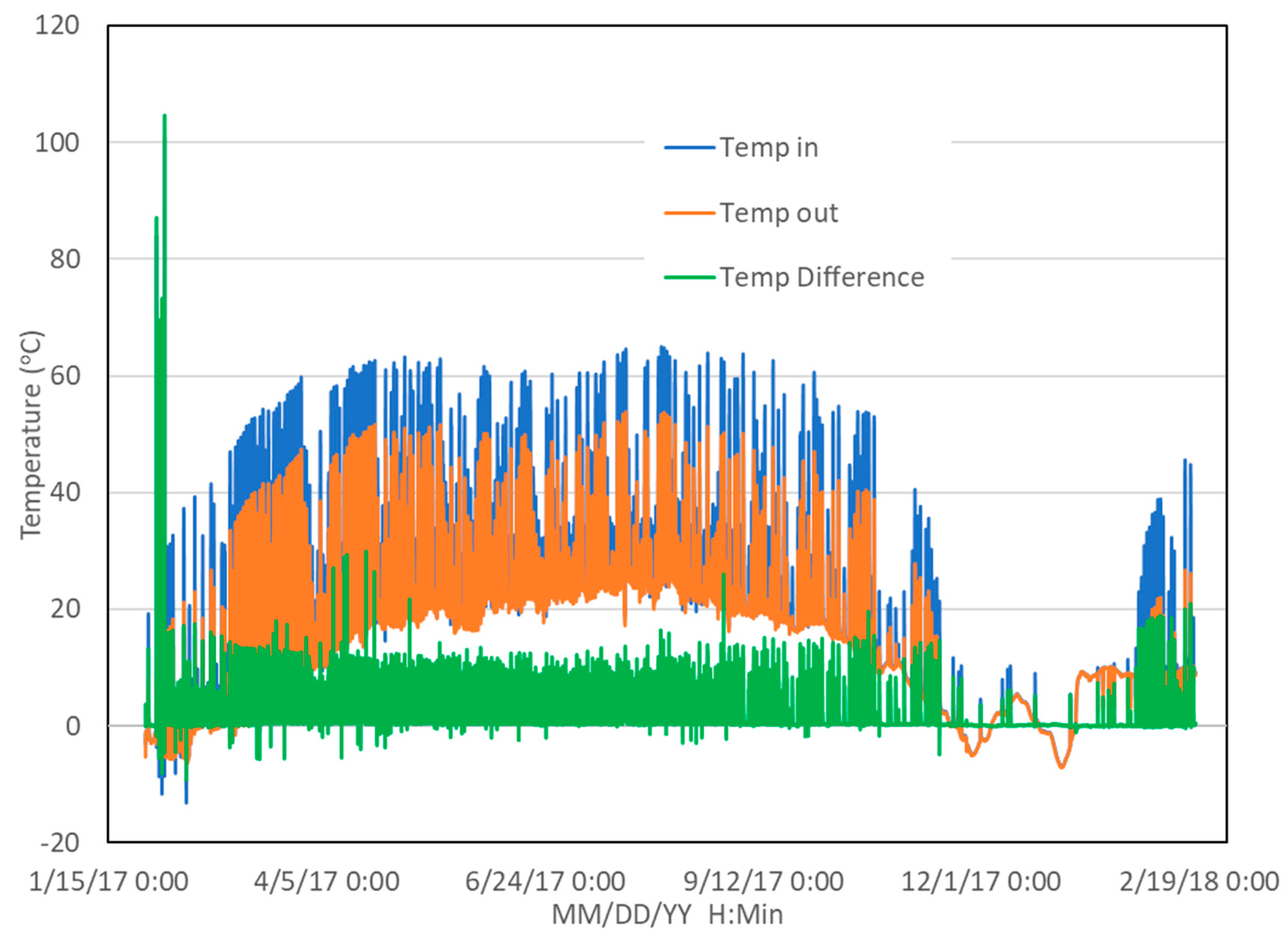
Glycol-water mixture return and supply temperatures to the thermal storage were recorded at 1-minute intervals with RTD sensor using the Caleffi DL3. Results are given in Figure 11. Initially, the pump flowrate was varied with exceptionally high and low flowrates. This was the period when the speed controller of the pump was being occasionally adjusted manually to establish a desired flowrate. The moderate flowrate established allowed for significant heat transfer while minimizing the pump’s power consumption. After a preferred pump speed was established, the flowrate was obtained to be 3.06 L/min (187 kg h⁻¹) of the glycol-water mixture through the thermal storage. It is observed that there were periods of extremely high temperatures before March. This was the time when the controller of the pump was occasionally varied to establish the desired flow rate. The total heating load of the garage, assuming an indoor temperature of 18 °C, was calculated. The heat obtained from the thermal storage was calculated. Then the reduction in heating load was computed, which was found to be 41.5%.

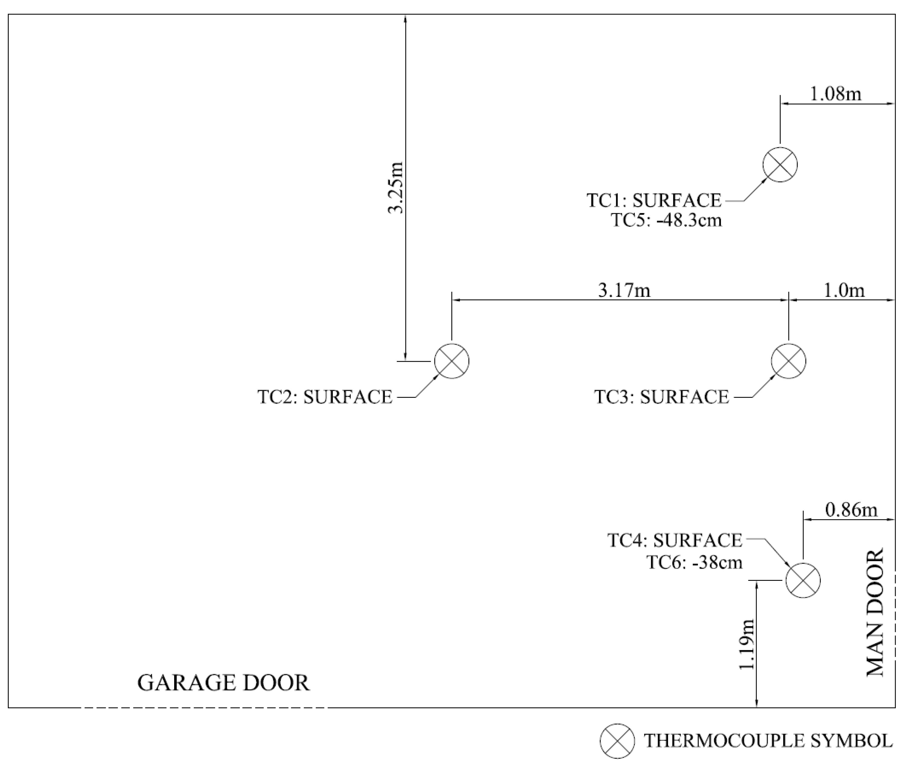
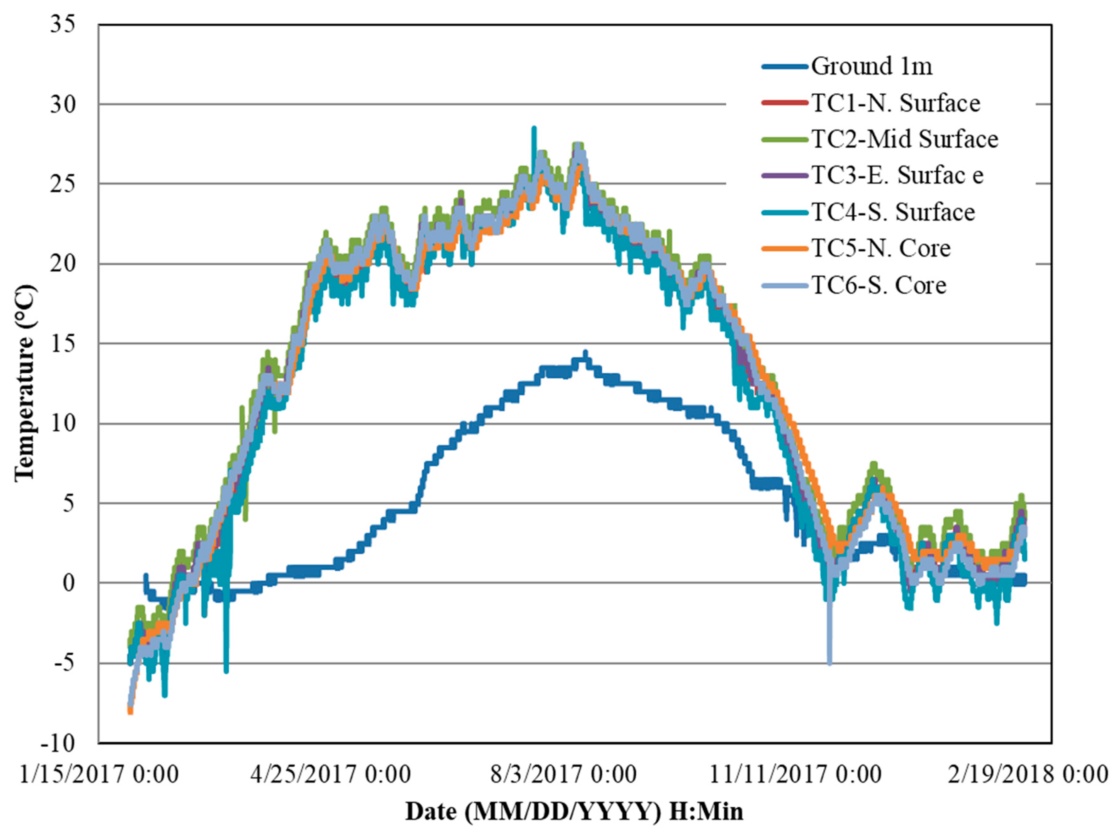
To obtain the profile of temperature in the thermal storage, temperatures were recorded at multiple points in the thermal storage every 15 min for the duration of the experiment.

Table 4. Average temperatures at different positions.

	TC1-North Surface	TC2-Mid Surface	TC3-East Surface	TC4-South Surface	TC5-North Core	TC6-South Core
Temp	12.5	13.5	12.7	11.9	12.9	12.8
Depth	-	-	-	-	0.48 m	0.38 m

gives the positions of the sensors and the average temperatures. The location of the thermocouples is shown in Figure 12. Figure 13 shows each sensors’ recorded temperature. The Figure shows that the core and surface temperatures overlap, indicating a uniform distribution of temperature throughout the thermal storage. Thermocouple number 5 (TC5) buried at a depth of 0.48 m and TC6 buried at a depth of 0.3 m showed average temperatures of 12.9 °C and 12.8 °C, respectively. These temperatures are comparable to those measured at the surface.

The south surface is a place where the temperature sensor was positioned closest to the garage man-door. This substantiates the higher temperature variations when work was done in the garage (frequent opening and closing of the man-door) during cold days. The average ground temperature, just below the insulation of the thermal storage at a depth of 1 m, was recorded to be 5 °C.

Numerical Simulation Result

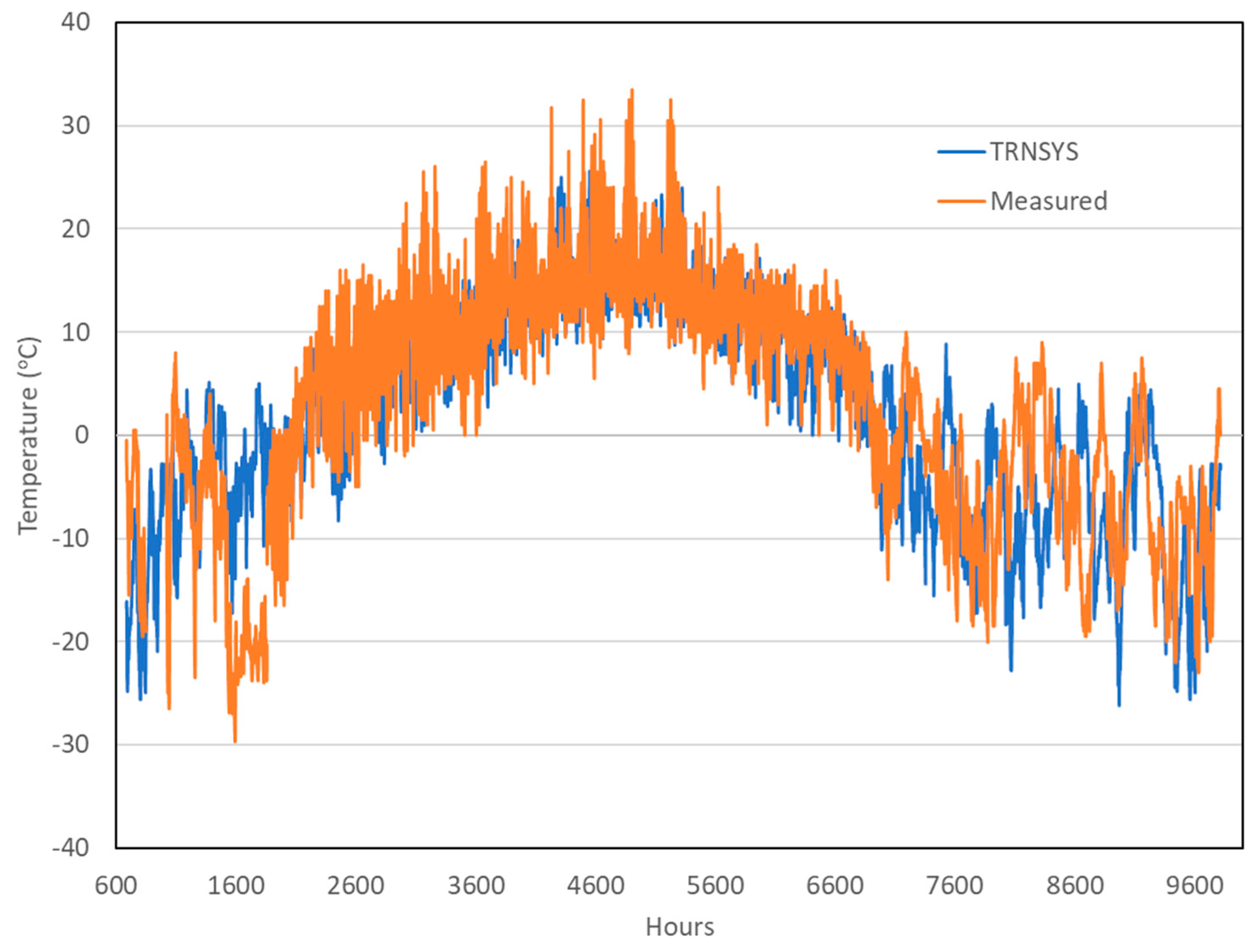
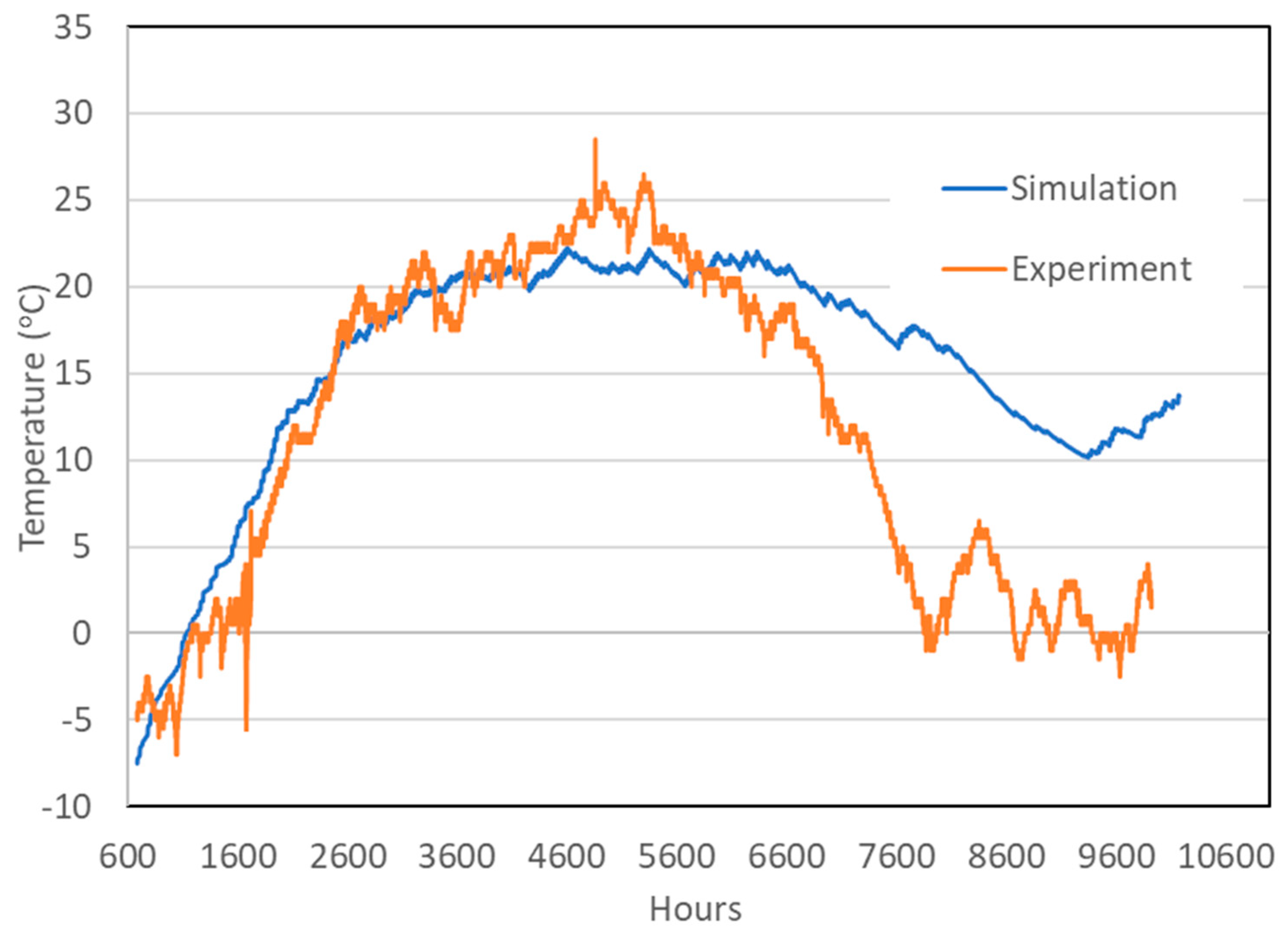
The numerically simulated temperature of the thermal storage for more than 1 year period time is compared to the experimentally measured one in Figure 14. Maximum observed garage temperature is ~28 °C. Maximum simulated temperature is ~22 °C. Also, close agreement was obtained between the simulated and the measured values from February to November. A significant discrepancy is observed between the measured and simulated values in December and January. During this period, while the actual garage temperature varied between 0 °C and 5 °C, the model predicted the temperature variation to be between 10 °C and 15 °C.

The reasons for this discrepancy could be: (1) the frequent opening and closing of the garage doors which was used as parking space as well as the frequent opening and closing of the man-door which could have contributed to the reduced garage temperature (measured) especially in colder December and January, and (2) the assumption of constant environment loss coefficient for the numerical simulation.

8. Conclusions

More than one-year monitoring results of seasonal solar thermal energy storage located in a very cold place with long period of freezing was presented. The studied house is in the city of Palmer, Alaska (~62° N, ~149° W). The most important contributions of this work can be concluded as follows:

• A detailed method for determining the thermal properties of the thermal storage was presented.
• The use of thermal storage was calculated to reduce the heating load of the garage by 41.5% under the given climatic conditions.
• Thermal storage systems made of readily available materials such as sand and pit-run can be a cost-effective way of storing thermal energy for Alaskan applications.
• In general, seasonal solar thermal storages are viable options in reducing the cost of energy in a region with extended freezing periods. This is significant for Alaska where the energy cost is 3-5 times the national average.